Can Vietnam Achieve One of its Millennium Development Goals? An analysis of schooling dropouts of children

(1)

T

HE

W

ILLIAM

D

AVIDSON

I

NSTITUTE

AT THE UNIVERSITY OF MICHIGAN BUSINESS SCHOOL

Can Vietnam Achieve

One of its Millennium Development Goals?

An analysis of schooling dropouts of children

By: Vo Tri Thanh And Trinh Quang Long

William Davidson Institute Working Paper Number 776

June 2005

(2)

CAN VIETNAM ACHIEVE

ONE OF ITS MILLENNIUM DEVELOPMENT GOALS?

An analysis of schooling dropouts of children

1

Vo Tri Thanh

Director of Department for Trade Policy and International Integration Studies, Central Institute for Economic Management (CIEM), Hanoi, Vietnam

Email: [email protected]

Trinh Quang Long

Researcher, Department for Trade Policy and International Integration Studies, Central Institute for Economic Management (CIEM), Hanoi, Vietnam

Email: [email protected]

Key words: Vietnam, education, MDGs JEL Codes: D10, I20, I29, C31

1_{Funding from the International Centre for the Study of East Asian Development (ICSEAD) is gratefully}

acknowledged. Without the ICSEAD’s support, this study could not be completed. The opinions expressed in this study are the responsibility of the authors and not of their organization, the Central Institute for Economic Management (CIEM).

(3)

Abstract

The objectives of this study are to identify the underlying determinants of the schooling dropout in Vietnam and to project its trend in the future up to 2015. Our examination is largely based on the three Vietnam’s Living Standard Surveys conducted in 1992/93, 1997/98 and 2001/02 and the conventional framework of educational investment at the household level.

The major determinants of the schooling dropout choice by households are found to be variables of child’s characteristics (such as age, working time, primary education, and number of siblings) and household economic situation (such as parental education, household’s per capita expenditure, and cost of schooling). In general, the effects of these determinants on the schooling dropout probability are statistically significant. In particular, the schooling dropout probability has been very sensitive to the changes in the household’s per capita expenditure and the direct costs of schooling, whereas recently the other determinants have had only minor impacts. In terms of schooling, girls have benefited more than boys did from their household's per capita expenditure increase, while they have suffered more than boys did from an increase in the direct cost of schooling. These differences, however, recently have narrowed substantially. The dropout situation is also regional specific and hence, a comprehensive approach is needed to deal with it. Moreover, at present the low quality of education is serious problem. Together with the parents' incorrect perception of and the community’s attitude to education values, this may increase the possibility of children’s schooling dropout. The dropout situation is also very much dependent on the public funding for education, which is still not effective in reducing the household current excessive financial burden and still biased against the poor regions.

The projection outcomes of the schooling dropout probability of children in the future up to 2015 is very much depending on the assumptions of the changes in the household’s per capita expenditure and the cost of schooling. When the growth rate of the cost of schooling is much higher (for example, by 1.2 percentage points) than that of the household’s per capita expenditure, the dropout rate would first decrease and increase again after 2010. The tentative assessments suggest that in these cases, there is a chance for Vietnam to achieve the national targets of the primary and lower secondary net enrolment rates in 2010. However, Vietnam could very hardly to achieve the MDG on the universal completion of primary education in 2015 and moreover, the achievements recorded by 2010 would be deteriorated. Regarding the scenarios, where the pace of changes in the cost of schooling is lower than that of the household’s per capita expenditure, the projections seem to provide a rather bright picture in terms of achieving the national education targets in 2010 and the MDG on education in 2015. The projections also show that there is a reason to be more optimistic about the elimination of the gender gap in education by 2010.

(4)

For a long time, education has been considered a mean for and a goal of development. Given the importance of education as well as Vietnamese people’s tradition of the fondness for learning, since the first day of the independence in 1945 the Government of Vietnam (GOV) has paid a great attention on education, especially on the elimination of illiteracy in the country. In September 2000, by ratifying the Millennium Declaration together with 188 other nations, the GOV committed itself to achieving the Millennium Development Goals (MDGs), including the universal completion of primary education by 2015 and the elimination of the gender disparity in primary and secondary education by 2005 and to all levels of education no later than 2015. To adapt the MDGs to fit local circumstances, the GOV also set several concrete goals of educational development in its Comprehensive Poverty Reduction and Growth Strategy (CPRGS). For example, the goal of the net enrolment in primary school is set to increased to 97% by 2005 and to 99% by 2010; the goal of the net enrolment rate in lower secondary school is set to increased to 80% by 2005 and to 90% by 2010; and the gender gap in primary and secondary education and the gap with ethnic minorities will be eliminated by 2005 and by 2010 respectively (UNVN 2003) 2.

Vietnam has recorded great achievements in education. In 1945, more than 95% of the adult population was illiterate. According to the data from the Vietnam Living Standard Survey 2001/02 (VLSS 2001/02), the general adult literacy rate was about 91% and over 94% woman below 40 years of age were literate. Vietnam has also developed a comprehensive education and training system including primary education, secondary education, college and university education, postgraduate education and vocational training. In comparison with other countries at the same level of GDP per capita, Vietnam has a much higher literacy index. In 2001, Vietnam’s

2_{In 2001, the levels of the net enrolment rates in primary and lower secondary schools were 92% and 67%} respectively. The ratios girls to boys in primary and lower secondary education were 99% in 2001 and 93% in 1998 respectively.Note that the GOV has set both the development goals directly and not directly based on the MDGs (such as reducing vulnerability, improving governance for poverty reduction, reducing ethnic inequality, and ensuring pro-poor infrastructure development) (UNVN 2003).

(6)

Human Development Index (HDI) 3 ranked at 109 among 175 countries, whereas its GDP per capita (in terms of USD PPP) ranked at 130 (UNDP 2003).

The Renovation (Doi moi) in 1986 and especially the market-oriented reform in 1989 marked a

turning point in the history of Vietnam’s economic development. Under the reforms, the education sector has experienced dramatic changes. On the one hand, opportunities for being educated are open for everyone. Many educational institutions have been established nationwide and the education system has become more diversified and democratized (Nguyen Thi Minh Tam et al 1998). More and more children have enjoyed a greater access to higher quality

education. On the other hand, a series of issues has emerged as a result of the change in the education system. As warning in the National Human Development Report 2001 (NCSSH 2001), Vietnam has to deal with “a number of major challenges" to education system, including school attendance, completion rates and general education quality. In order to achieve the educational development goals, it is very important to further integrate ethnic minorities and children from vulnerable families into the formal education cycle and to improve completion rates (UNVN 2003). In other words, it is require not only to get all the children into school but also to keep them in schools.

There were some studies attempting to discover determinants of schooling dropout in Vietnam4. These studies, however, suffer either from old data collected only up to 1998 or from lack of variables, which may be influenced by policy arrangements such as skews of government expenditure for education sector. A prompt and comprehensive analysis exploring how factors at the micro level (household level), at the meso level (community level) and at the macro level (economic policies, especially public spending) interactively affect the decisions of household to withdraw their children out from school system), increasingly emerges as a necessary requirement for government policies to be adjusted in order to achieve its goals.

The major objectives of this study are to fill the current gaps in understanding the dropout trend in Vietnam since the early 1990s and its determinants and to stimulate the dropout trends in

3_{According to the UNDP (various issues), the HDI is based on three basic indicators: longevity}

(measured by life expectancy at birth); educational attainment (measured by a combination of adult literacy and the combined gross primary, secondary and tertiary enrollment ratio); and standard of living (measured by real GDP per capita adjusted according to purchasing power parity). The higher the HDI of a country is, the better its human development is evaluated.

(7)

Vietnam in the future up to 2015. Then the study can give some backgrounds for the evaluation of the possibility of achieving Vietnam’s educational development goals and for the suggestion of some relevant policy implications.

The analysis of the determinants of dropout is based on a conceptual framework containing elements of the conventional theories of educational investment at the household level. The econometric techniques of the probit models are applied for estimating the magnitudes and significances of the determinants of schooling dropout at three different time points, namely

1993, 1998 and 2002. The sources of data for estimations are from the Vietnam Living Standard Surveys (VLSS) conducted in 1992/93, 1997/98 and 2001/02. The same kind of probit model can also be estimated for the pooling data from three VLSSs and then, it can be used for the stimulation purpose.

The remainder of the study is structured as follows. Section 2 lays out an analytical framework for analyzing how the household makes decisions regarding their children's education. Section 3 reviews the schooling trends and the dropout situation in Vietnam during the period 1993-2002. In this section we also attempt to highlight the causes of schooling dropout through some stylized facts and observations. Section 4 presents the estimations of the probit models to reveal the factors determining the choice of children’s dropout. In addition, this section also projects the children’s dropout rates in the future up to 2015 based on several scenarios. Section 5 concludes the study with a brief summary of our key findings and some policy implications.

2. AN ANALYTICAL FRAMEWORK AND INTERNATIONAL EMPIRICAL EVIDENCES

Education is widely regarded as both consumption good and an investment good. Parents educate their children because they enjoy having literate and well-educated children. Parents also invest in their children to ensure that their offspring will support them later in life. In this section, a standard model of parental and household decision-making regarding children's education is studied. The model basically follows one studied by Glick and Sahn (2000). This section also

4_{See, for example, Vo Thanh Son}

(8)

highlights some international empirical works supporting for the key conclusions from the model.

2.1. A theoretical model of educational investment

In this model, parents are viewed as the principle while their children are viewed as agents. Parents determine the educational level of their children. Also, households are viewed as "unitary" households, i.e. preferences of parents are identical or if their preferences are not the

same, the household is assumed to act as if they were maximizing a single utility function. Consider a household consisting of a father, a mother, and N children, among them m children are daughters and n children are sons (m+n=N). Parents are considered to live in two periods. In the first period, they work and raise their children. They will retire in the second period. In the first period, household consumption is total income after subtracting a proportion to invest in their children's schooling. Consumption in the second period depends on the remittances of their children's income, which in turn partly depends on the children's level of education obtained in the first period. In their schooling decisions, parents must trade off their current consumption (reflected by investment in children's schooling) against their future consumption and their children's wealth. The identical preference of parents is formally represented by a utility function as follow:

U=U(C

1

, C

2

, Y

d1

, ..., Y

dm

, Y

s1

, ..., Y

sn

)

(2.1)

in which, C1, C2 denote household (parental) consumption in the first and second period

respectively; Ydi with i=1,…, m and Ysj with j=1,…,n correspondingly denote the incomes

generated by the ith daughter and jth son in second period. This model can be specified in more detail as follows:

)

....,

,

,....

,

(

)

(

C

₁

G

C

₂

Y

_d_,₁

Y

_d_,_m

Y

_s_,₁

Y

_s_,_n

F

U

=

+

(2.2)

If the parents do not explicitly prefer one gender-specific child to the others, then for any kth and lth children

∂

G

/

∂

Y

k

=

∂

G

/

∂

Y

l and

∂

G

/

∂

Y

k

∂

Y

k

=

∂

G

/

∂

Y

l

∂

Y

l

2 2

when Yk = Yl.

It is further assumed that the amount of children’s income remitted to parents is proportional to each child's income. Children's income in the second period in turn depends on the level of

(9)

schooling attained in the first period as well as child-specific variables Z such as sex, birth rank, etc. As parents' consumption in the second period depends on the transfers from their children’s income, we can have a formal second period parental consumption:

∑

= = + = n j sj j m i di iY Y C 1 1 2 β γ (2.3)

where βi is the rate of transfer per unit wealth from the ith daughter and γj is the rate of transfer

per unit wealth from the jth son.

Children's income depends on their level of schooling attained as well as their specific characteristics and hence, it can be formally presented as below:

di i di

b

S

Y

=

and

Y

sj

=

g

i

S

sj (2.4)

in which Sd,i with i = 1...m and Ss,j with j = 1...n are the education of the ith daughter and jth son; b

and g are the respective monetary returns to investment in human. The monetary returns to schooling investment also reflect gender of the child.

It is also assumed that in the first period, parents spend their total available time in the labor market while the time of children is divided between work and schooling. We have the household's full income constraint as below:

∑

= = = = + + = − + − + + + n j s m i d n j s sj sj m i d di di f f m mw T w T S w T S w C PS i PS j T V 1 1 1 1 * 1 * ₍ ₎ ) ( (2.5)

The left-hand side of Equation (2.5) represents the total income of household in the first period, while the household's expenditure is on the right hand side. V denotes unearned income. Tm, Tf

are total time that mother and father, respectively, work in the labour market. Tdi, Tsj are the time

that the ith daughter and jth son have, thus (Tsj-Ssj) and (Tdi-Sdi) are the time that the ith daughter

and jth son devote to income generating activities. Wm, wf, ws*, sd* are their wage rate

respectively. P is the direct cost of education, which includes tuition fees, books, uniforms, etc. We assume that the cost of education is assumed to be identical for all grades and for both sexes.

(10)

Equation (2.5) shows that the cost of education consists of two components: the first ( i d PS for ith daughter or j s

PS for the jth son) is the direct cost and the second is the indirect cost that children have foregone when attending school.

Parents choose Sdi and Ssi to maximize their utility subject to the full income constraint and the

constraints relating earnings to schooling and parental consumption to child earnings. By substituting Equations (2.3), (2.4), (2.5) into Equation (2.2), the following maximization problem is derived: } ] ) ( [ ] ) ( [ { max 1 , * , 1 * * , , ,

∑

₌

∑

₌ + − + + − + + + = n j j s s s sj i d m i d d di f f m m s Sdi d jU F V T w T w T w P w S T w P w S } ...., , , ,... , ), {( ₁ ₁ ₂ ₂ ₁ ₁ ₂ ₁ 1 1 sn n s s dm m d d n j sj j j m i di i ibS g S bS b S b S g S g S g S G

∑

= = + +

β

γ

(2.6)

Solving this maximization problem results in a reduced-form equation that shows the demand for quantity of daughters' and sons' schooling as following:

S

di

= S

di

(w

m

,w

f

,V,P,S

m

,S

f

,Z

di

, Z

sj

, H) and

S

sj

= S

sj

(w

m

, w

f

, V, P, S

m

, S

f

, Z

di

, Z

si

, H)

(2.7)

These equations are functions of the price of education, wage rates of parents, child-specific characteristics of all children (Zdi and Zsj with i = 1...m, j = 1..n), unearned income, parents'

education and other household (and community) factors (H).

2.2. Model implications

The maximization problem can be used for deeper examination of how "unitary" parents invest in their children's education. If an interior solution is assumed (Sd,i and Ss,j > 0 with i = 1..m and j

= 1…n), the first order conditions (FOC) could be derived. For each daughter i, the first order condition is i i d i i d

b

Y

G

b

C

G

w

P

C

F

, 2 * 1

)

(

∂

+

∂

=

+

∂

_β

( 2.8)

(11)

j j s j j s

g

Y

G

g

C

G

w

P

C

F

, 2 * 1

)

(

∂

+

∂

=

+

∂

_γ

( 2.9)

Thus, parents invest in their children's education to the point that the marginal cost in terms of consumption in the first period equals the future marginal benefit. These marginal benefits are equal to the marginal utility of second period consumption multiplied by the remittance rate per unit of education (reflected in the children's wealth) plus the utility the parents derive from a marginal increase in the children's wealth, hence children's education.

Turning to the implication of the model for the resource allocation between children, in general, and between genders, in particular. If the market returns to the one child are higher than those to the other children, parents will invest more in that child's education since the utility of parents will increase due to increase in their consumption in the second period and due to higher total wealth of all their children. A similar conclusion could be derived when the rate of remittance of any child is larger than the others, or if parents are more concerned with any child's wealth than with other children's wealth.

If the wage rate of daughters and sons are equal, children’s sexes do not matter in analysis. For children kth and lth , the parents will invest in their education to equalize their marginal benefit, i.e. l Y G l C G k Y G k C G l l k k ∂ ∂ + ∂ ∂ = ∂ ∂ + ∂ ∂

_α

_δ

2 2 (2.10)

where αk, δl denote the rates of remittances, while k and l represent the monetary returns to

investment in education of the kth and lth children respectively.

If k>l, the left hand side of Equation (2.10) is greater than the right hand side when evaluating at the same level of education. Since the marginal benefits to education are a decreasing function of education, Equation (2.10) is only satisfied at a point where Sk>Sl. When αk>δl or when

l k G Y

Y

G ∂ >∂ ∂

∂ , the marginal benefits from the kth child's education is higher than the marginal benefit from the lth child's education, given that the educational levels of these two children are equal. By a similar argument, investment in the kth child's education is higher than investment in the lth child.

(12)

Some assumptions are made before studying the effects of changes in family factors. Firstly, it is assumed that there are two children, the lth child and the kth child. These children are either girls, or boys or a boy and a girl. Secondly, the monetary returns to education of the lth child are higher than that to education of the kth child, i.e. l>k.

Price elasticity will be investigated first. Given that the wage rates for the lth child and kth child are unchanged and equal, an increase in the direct costs of education will raise the marginal cost of education investment - that is, the left hand side of the FOC equations for these two children. In this case, the assumption of l>k implies that the change in Sk that restores the equilibrium

condition in the FOC equation for child k for each level of Sl is larger than the change in Sl that

satisfies the lth child's FOC equation for each level of Sk. That is the demand for education of the

child with lower monetary returns to education is more price elastic than that of the child with higher monetary returns. Alternatively stated, when l>k, the marginal benefit from the education of child l decreases faster with S than does that from the kth child's education. Hence the

adjustment necessary to restore equilibrium is less with child l than child k. Thus, when the price of education increases, the child with lower monetary returns will suffer from larger reduction in educational investment than the child with higher monetary returns. Similarly, in the case that the rate of remittance in the second period of child l is higher than that of child k, the demand for

education of child l is less price elasticity than that of child k.

In the case that the current wage rate of child k increase while that of child l and direct cost of

education are unchanged and l is still higher than k (in addition, keep in mind that wage rates of

these two children are assumed to be identical). The marginal cost of education of child k is now

higher than that of child l. In this case, changes in Sk is required to restore the equilibrium

condition of the FOC equation for child k while the equilibrium condition of the FOC equation

for child l is in comparison with demand for education of that child before increase in current

wage rate .

Things become more difficult when (1) the current wage rate of child l increase and that of child k is unchanged, or (2) current wage rates of both children increase but that of child l is higher than that of child k. If the monetary returns to education of child k is still lower than that to education of child l, the demand elasticity with respect to changes in current wage rates will depend partly on how large the differences between the monetary returns to education of child l

(13)

and child k and partly on how different between the remittance rates of child l and child k. If these differences are large enough to offset the effects of changes in current wage rate, there will be not affect the demand for educational of both children.

Similarly, an increase in the income affects the first order conditions through the marginal cost of educational investment, i.e. the left-hand side of the FOC equations. This increase reduces the marginal utility of current consumption and therefore lowers the marginal cost. This fall in marginal cost is similar to a reduction in direct cost of education. Therefore, a rise in income leads to a greater increase in the investment in education for children who have lower monetary returns to education. Alternative stated, the demand for education of children with lower monetary returns to education is more income elastic that that of children who have higher monetary returns.

This model also implies that the price elasticity of demand falls with income and that a price elasticity of children with lower monetary returns to education falls faster with income than that of children with higher monetary returns to education. An increase in income lowers the marginal utility of current consumption and therefore, the marginal cost of human capital. This result implies that a rise in prices represents a larger increase in marginal cost at lower levels of income than at higher levels of income. Hence, increased prices will generate larger reductions in educational investment among families with lower incomes than among families with higher incomes.

Given production techniques in rural areas, gender of children will partly influence the opportunity costs of children, which, in turn, affect the probability to continue their schooling paths. In developing countries, it is potential that the opportunity cost of educating girls is higher than that of boys. Girls are typically demanded to perform more housework than boys, reflecting cultural or social attitudes toward the proper economic role of women and girls. Given these attitudes, the marginal cost of girls' time will be higher than boys', and consequently their demand for education will be lower as we have analyzed above. However, in some cases, the demand for boys' time is higher than that for girls'. In fact, the demand for gender-specific children's time depends on the production technique of household, which is assumed to be exogenous in this analysis.

(14)

For the same reasons, it would be expected that certain changes in household structure will affects daughters' schooling more strongly than sons'. An increase (assumed exogenous) in the number of very young children will raise the demand for the labour of girls in childcare in the home. In other words, under this circumstance, the opportunity cost of girls' education is higher than that of boys. Thus, their likelihood to be dropped out will increase. By the same logic, additional older siblings or presence of grand parents especially grand mother may reduce the opportunity cost of a daughter's time by providing substitutes for household work or through economics of scale in household production, thereby reduce the likelihood to be withdrawn from school.

Gender of children will determine not only their opportunity cost but also their potential monetary returns to education in the future. Women are usually discriminated in the labour market even in developed countries in terms of access to employment or of earnings; the monetary benefit to their education, thus, is lower than that to sons'. In fact, there may be substantial returns to female schooling in non-market production, but parents may not be aware of these non-monetary benefits or may value them less than monetary ones. Even if educated girls go on to work and receive earnings on a par with men, income remittances to parents from married adult daughters, who join their spouses' families, may be lower than from adult sons. If that is not the case, i.e. the remittance rate is equal for both sons and daughters, the returns to parents from educating girls could be low. This could be explained by potentially lower quality of daughters' education than that of sons', which reflected regular interruptions in attendance or schoolwork resulting from household obligations.

Age of children will be considered in the parents' process of making decision on whether or not withdrawing them from schools. In rural production, the older children tend to have higher opportunity costs (larger foregone earnings) as well as higher direct cost of schooling (higher direct costs required higher grades), which increase the marginal cost of education, and hence in order to restore the equilibrium condition the resource used for investment in education for older children will be cut partly. This also means that the older children will face a higher chance to be withdrawn from school.

Parental education is expected to be positively associated with children's schooling. Educated parents are more able to assist in their children's learning, raising the returns relative to less

(15)

educated parents, and are also more likely to recognize the benefits of schooling. Positive parental schooling impacts are also expected from a schooling as a consumption good perspective, since better educated parents are believed to enjoy educated children more than less educated parents; thus mother and father education will act as a taste-shifters in the schooling demand functions.

Now we will examine how these factors affect children's education investment within the framework of the collective household model. The model predicts that factors that raise the

bargaining power of the wife should increase allocations to goods she prefers (The mother's education stands out as such factor for which our dataset provides information). Women with more schooling are able to earn more, improving her power in bargaining position and (if they are actually working) the level of income under their direct control. Thus, if women value the schooling of their children more than men do, maternal schooling will have stronger impact than parental schooling on children's education. Further, mothers may prefer to allocate more resources, including for human capital, to daughters while fathers prefer sons5. Then increases in mother's schooling would have a larger beneficial effect on daughters' education than on sons', and father's schooling would favour sons' education (same-sex effect and cross-sex effect). The former is particularly plausible because the mother's bargaining power and her preferences for daughters' schooling are both likely to rise with her own education.

From the above analyses, we see that the relationships of maternal and child schooling are the same in both models. Under a bargaining framework, a larger maternal education impact on daughters' education than sons' may reflect maternal preferences for educating girls. In the unitary household model, households in which the mothers have high educational level also have strong common preferences for daughters' schooling. However, under the unitary household model, the problem will arise because of martial sorting: some husbands, especially educated men, will choose wives who are well educated or even better educated. This reflects their preferences for educated women hence for daughters' schooling. This problem results in heterogeneity in preferences between households rather than within household.

5_{This does not mean that fathers love their sons more than their daughter, even in some cases, fathers}

express their love to daughter much more than to sons. However, as rationally economic agents, fathers prefer to invest in their sons.

(16)

2.3. International empirical evidences

There have been a number of studies trying to explore the determinants of children's attainment. Most of studies related to determinants of children attainment, in general, and children's education, in particular, have viewed the process of children's attainment to be sequential choices made by family, which is considered as a production unit which employs real inputs to generate utility for its members (Haveman and Wolfe 1995). Most of these studies assumed that decisions makers in households are parents and they share a common utility function. Parents in these models act as children's gatekeepers through their control over children's access to educational resources made available by the Government and community (Lloyd and Blank 1996). Thus, children's attainment is influenced by choices made by parents regarding the amount of family resource allocated to children, the timing of their distribution, the number of children, etc.

Concerning measurement of educational attainment, a variety of measures have been studied. These measures include categorical dummy variables (whether the child graduate from a certain level of education) and continuous variables, indicating the extent of attainment (annual earnings), depending on the issues to be addressed.

Reduced form equations for the dependent variables of interest are widely estimated using methods ranging from OLS techniques (for studies related to years of schooling such Datcher (1982) or Duncan (1994), to binomial probit (for studies exploring categorically educational attainment), and to Heckman two-step procedures (Cockburn 1999). However, the reduced-form approach is preferable to the alternative of including the endogenous variables without suitable instrumentation, which can lead to biased and inconsistent estimates.

The determinants of children's educational choices can be grouped into three main categories: individual, household and community characteristics. Among which variables describing parental characteristics or choices are the most commonly used in studies of children's educational attainments? In fact, parents with immediate costs and longer-run returns in mind, will make decisions regarding children's schooling.

Parental human capital, measured by the number of years of schooling attained, is the most fundamental economic factor. The empirical studies have shown that in general this factor is statistically significant and quantitatively important for children's education and for children's

(17)

decision to withdraw from schools, no matter how it is defined. The human capital of the mother is usually more closely related to the attainment of the child than is that of the father.

The family's income level in which a child grows up is perhaps the best measure of the level of economic resources devoted to the child by the parents. However, income variable may be a rather crude proxy of the economic resources available to a child. Often family income is recorded only in a single year, and hence measures permanent income with error. And it may convey little about family allocation of income to children and fail to capture other economic resources devoted to the child (Haveman and Wolfe 1995). Most of studies have employed the ratio of the income level of the family to the income needs of the family, reflecting its size and structure. Family's income is positively associated with the educational attainment of the child, and the variable is statistically significant in many studies that found out a positive association. Income variability may lower children's educational attainment since it may be accomplished in part through increased child labor participation, thus reduced educational participation. Jacoby and Skoufias (1997) found that rural Indian households adapt to negative income shocks by reducing school attendance and increasing labour participation among their children as a form of self-insurance.

The effects of family structure and the extent of mother's work on children's education have regularly been studied. Growing up in a one-parent family (or experience divorce or marital separation) is negative related to the level of school attained and is statistically significant. Evidence on the effects of mother's work on children's educational choices is mixed.

Other variables related to parental investments such as the number of geographic moves during childhood, the number of siblings, religiousness have been found to have statistically significant and quantitatively large effects on children's educational attainment.

Children's characteristics also affect their own educational attainment. Most empirical work study boys and girls separately and do not directly test the role of sex (Cockburn 1999). In the cases, where pooled data were run with a boy dummy, it had a positive effect on children's education attainment.

Canagarajah and Coulombe (1997) specifically tested also the relationship between school and work participation in a simultaneous equation model. They found that the relationship is negative

(18)

and significant. Thus factors that reduce child labour participation would increase school participation.

The relationship between child's age and child's schooling attendance are negative in most of studies. However, this relationship is not simply linear. Admassie (2002) found that the probability of going to school increases with age and decreases with its square, suggesting an inverted U-shaped relationship.

In addition, community characteristics also are found affecting the children's attainment. Many studies use schooling characteristics as proxy for community characteristics and find that presence, proximity, and quality of local schools should have positive effects on school participation while the impact of school costs should be the opposite.

3. EDUCATIONAL CHANGES AND SCHOOLING DROPOUT SITUATION IN VIETNAM

As mentioned in Introduction, the Renovation, especially the market-oriented reform since 1989, has resulted in the dramatic changes of education system in Vietnam. This section gives a brief overview of Vietnam’s economic reform, performance and educational changes. Then the section reviews the dropout trends in Vietnam during the period 1993-2002 (based on the three VLSSs). It also attempts to look at the possible causes of the schooling dropout situation.

3.1. An overview of Vietnam’s economic reform, performance and educational changes6

Prior to the 1980s, Vietnam’s economy was essentially a centrally planned economy at a low development level. Economic reform in Vietnam was initiated in the early 1980s. However, only the Renovation (Doi moi) in 1986 and especially the radical market-oriented reform of 1989

marked a turning point in the history of Vietnam’s economic development. In March of 1989, Vietnam adopted a radical and comprehensive reform package aimed at stabilizing and opening the economy, and enhancing freedom of choice for economic units and competition so as to change fundamentally the economic management system in Vietnam. The measures undertaken hereafter included:

6_{Overview of the economic reform process is largely adapted from Le Dang Doanh}

(19)

- Almost complete price liberalization;

- Large devaluation and unification of the exchange rate; - Increases in interest rates to positive levels in real terms;

- Substantial reduction in subsidies to the state-owned enterprises (SOEs);

- Agricultural reforms with the replacement of cooperatives by households as the basic decision-making unit in production and security of tenure for farm families;

- Encouragement of the private sector, including foreign direct investment (FDI); - Removal of domestic trade barriers and creation of a more open economy.

Despite broad and fast liberalization, it was recognised even in 1996 that significant restrictions remained, for instance in the areas of trade and market entry. The reforms of the SOEs and the financial sector have been limited and not keeping pace with economic development. There has also been a deep concern with the question of sustainable economic growth and development, especially during and after the Asian crisis in 1997-98. The challenges and difficulties facing Vietnam had called for further Renovation process. However, in general during 1997- 99, Vietnam was reluctant to undertake a decisive and comprehensive reform program. The years of 2000-03 witnessed the implementation of the demand stimulus policy to revitalize the economy and the new stronger commitments to reform continuation. Some significant progresses were made, especially in the development of private sector and trade liberalization. Meanwhile, the reform of the SOEs, banking system, and public administration were slower than expected and this limited the effectiveness and efficiency of other reforms. In general, the reforms have accelerated somewhat but with uneven performances.

(20)

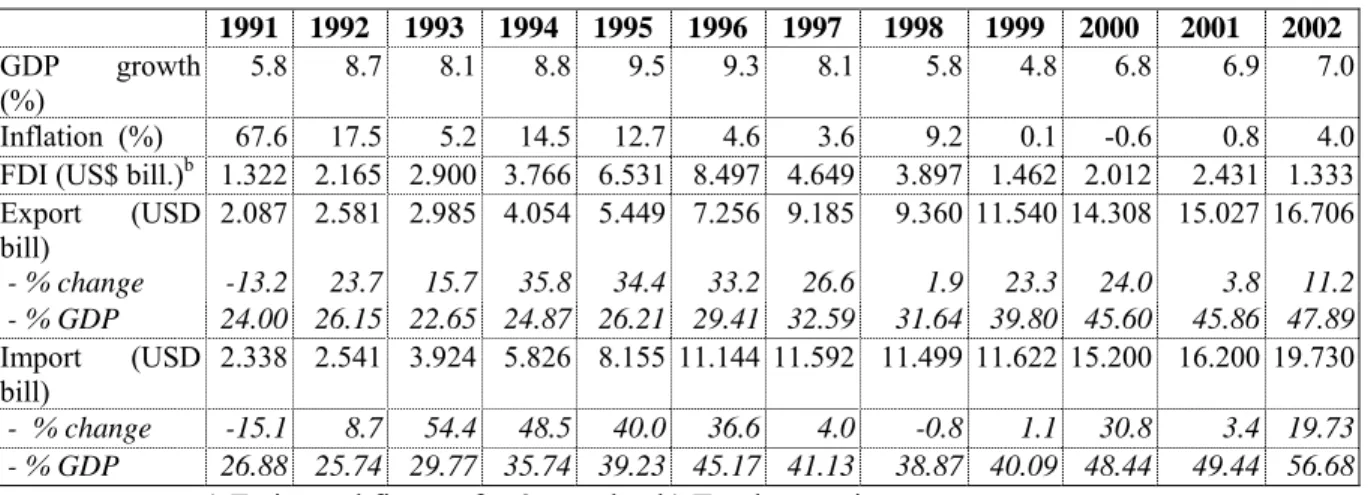
Table 3.1: Some macroeconomic indicators, 1991-2002 1991 1992 1993 1994 1995 1996 1997 1998 1999 2000 2001 2002 GDP growth (%) 5.8 8.7 8.1 8.8 9.5 9.3 8.1 5.8 4.8 6.8 6.9 7.0 Inflation (%) 67.6 17.5 5.2 14.5 12.7 4.6 3.6 9.2 0.1 -0.6 0.8 4.0 FDI (US$ bill.)b _{1.322 2.165 2.900 3.766 6.531 8.497 4.649} _{3.897 1.462 2.012 2.431 1.333} Export (USD bill) 2.087 2.581 2.985 4.054 5.449 7.256 9.185 9.360 11.540 14.308 15.027 16.706 - % change -13.2 23.7 15.7 35.8 34.4 33.2 26.6 1.9 23.3 24.0 3.8 11.2 - % GDP 24.00 26.15 22.65 24.87 26.21 29.41 32.59 31.64 39.80 45.60 45.86 47.89 Import (USD bill) 2.338 2.541 3.924 5.826 8.155 11.144 11.592 11.499 11.622 15.200 16.200 19.730 - % change -15.1 8.7 54.4 48.5 40.0 36.6 4.0 -0.8 1.1 30.8 3.4 19.73 - % GDP 26.88 25.74 29.77 35.74 39.23 45.17 41.13 38.87 40.09 48.44 49.44 56.68

Note: a) Estimated figures for 9 months; b) Total commitments Source: GSO (various issues) and authors’ estimates

Thanks to the Renovation and especially the market-oriented reforms, Vietnam escaped from crisis in the mid-1980s and the face of Vietnam’s economy and society has changed significantly (Table 3.1). From 1990 to 1997, the GDP growth rate was maintained at around 8% per annum on average. The GDP growth rate, however, went down between 1997 and 1999, partly because of the Asian financial crisis, and partly because of the dissipation of reform effects. Since 2000, the economy has regained its high growth rate at around 7% per annum.

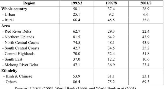
Successful economic development has resulted in overall improvement of people’s welfare and significant poverty reduction irrespective of measurement methods. The food poverty incidence in Vietnam reduced from 25% in 1993 to 15% in 1998 and 11% in 2002, while the total poverty incidence, which is measured by adding the minimum non-food expenditures to the amount of the food poverty line, also declined from 58% to 37% and 29% respectively over these same years (SC 2003). That means that Vietnam has met well ahead of schedule the MDG target of halving poverty rates between 1990 and 2015. Vietnam has also achieved notable results in human development. There has been a significant increase in Vietnam’s (from 0.623 in 1994 to 0.688 in 2001, and correspondingly, the Vietnam’s rank has been improved from 121 to 109). Vietnam now ranks 5th among the ASEAN countries, after Singapore, Malaysia, Thailand, and Philippines (UNDP 2003).

The progress in poverty reduction, however, is still fragile and several problems of poverty need to be addressed. First, around 95 percent of the poor are now living in rural areas, a higher share

(21)

than that of 90% in 1998. Second, the poverty situation has spread unevenly among regions and poverty is deepest in the areas with high ethnic minority populations such as the Northern Uplands, the Central Highlands and the North Central Coasts. Third, the gap between rich and poor has tended to widen. The Gini coefficient for consumption expenditure went up to 0.37 in 2002 from 0.35 in 1998 and 0.33 in 1993. Moreover, the real expenditure per capita of the richest 20 percent of households in Vietnam in 2002 is some 6 times higher than that of the poorest 20 percent, up from some 4.6 times higher in 1993 (UNVN 2003). It seems to be that the lower the poverty incidence, the harder the poverty reduction (Table 3.2). This could be the case since fighting against “hard-core” poverty needs to be undertaken under a more comprehensive framework, implying an increasingly important role of the specific programs targeted on the poverty reduction.

Table 3.2: Poverty Incidence by Regions

Region 1992/3 1997/8 2001/2

Whole country 58.1 37.4 28.9

- Urban 25.1 9.2 6.6

- Rural 66.4 45.5 35.6

Area

- Red River Delta 62.7 29.3 22.4 - Northern Uplands 81.5 64.2 43.9 - North Central Coasts 74.5 48.1 43.9 - South Central Coasts 42.7 34.5 25.2 - Central Highlands 70.0 52.4 51.8

- South East 37.0 12.2 10.6

- Mekong River Delta 47.1 36.9 23.4

Ethnicity

- Kinh & Chinese 53.9 31.1 23.1

- Others 86.4 75.2 69.3

Sources: UNVN (2003), World Bank (1999), and World Bank et al (2003)

The GOV and Vietnamese people have traditionally accorded high priority to education. The right of all children and adults to education constitutes a central pillar of Vietnam's education law and Vietnam has devoted considerable efforts and resources to the realization of this right. The investments in education, much of which predates even the launch of market-oriented reform, have resulted in remarkable achievements in education. Together with the economic reforms,

(22)

however, the education sector has also experienced dramatic changes, especially in terms of financial provision and private participation.

The education and training establishments finance their operation via two financial sources: the State budget (including Central State budget, provincial budget and Official Development Assistance ODA) and the revenues raised by themselves. The responsibility of funding by State budget is divided between different levels of government7. The second financial source includes such items as tuition fees, other contributions by students/their parents and voluntary contributions by various donors.

Regarding the State budget, the share of funding for education and training in terms of GDP increased from 2.2% in 1993 to 3.2% in 2001. The proportion of funding for education and training in total budget expenditures also increased significantly, from 9.5% in 1993 to 11.9% in 20018. However, the education and training budget has been concentrated on the current expenditures, which largely cover teachers’ salaries. For example, in 2001, 81% of the total

education and training budget was spent on current expenditures while the remaining, 19% was left for spending on capital construction and on curricula and goals education and training9. The budget constraints are hindering a considerable improvement of the quality of education and training system in Vietnam.

Population has been used as a dominant criterion in allocation of the public resources to education sector. While this criterion ensures the simplicity for resource allocation, it may not totally reflect the true need for public funding for education. A number of other criteria such as the number of students in an area, or the proportion of illiterate population, or of ethnic minorities, or the condition of education facility, should also be important. The empirical study by Vu Quoc Ngu (2004) shown that, as expected, population has significant and positive impacts on the public spending on education. At the same time, number of students and proportion of

7_{The central government is responsible for the funding for the universities and colleges and the}

vocational training schools as well as the national programs such as “Education for all”. The provincial governments are responsible for the funding for upper secondary schools. The district governments take care of the funding for lower secondary schools and all primary schools. Kindergarten and nursery are within the financial responsibility of the communes’ authorities.

8_{Authors’ estimation based on the data in GSO (various issues). The goal of education and training}

(23)

population with no degree have significant, but negative relations with the level of the public

spending on education. Moreover, the variables such as proportion of illiterate population, share of ethnic minorities in population, teacher class ratio, and distance from commune centre to school, have no bearing on the level of public spending on education. In other words, the criteria currently being used in the allocation of the education funds needs to be reviewed.

The division of the responsibility between different government levels and the current criteria used for allocating the public resources to education sector also favour the rich areas. Although the South East and the Red River Delta regions rank first and third on per capita GDP, they rank first and second on per capita public expenditure on education and training. Moreover, in general, the poorest 20% receive just over 10% of the total public funds (delivered mostly through primary education), while the richest 20% receive more than 35% (delivered through lower, upper secondary and higher education).

Regarding the other sources of funding, in an effort to reduce financial burden, in 1989 the GOV introduced tuition fees with only exemption given to the primary education (Le Bach Duong 2000). Generally, households have to pay two types of charge/fee: official tuition fee and informal charge. The official charges calculated on a per child basis, are flat and hence, create a greater burden per child for poor families than rich ones. The regressive nature of the charges increases as the amount of the charges increases.

While official tuition fees are low, the informal charges, set either at the central level or at the local level of school or commune, are fairly high for parents. However, this charge differs among families living in rural and urban areas and among educational levels. Table 3.3 reveals that richer families can afford much higher spending for education than the poorer ones. For example, on average the richest families spend for their children in primary education 5.8 times more than the poorest families do. Given the public resource limitation, the private spending can have a significant positive impact on the education quality. Thus, the students in the rich families can access to education with much better quality. As the poor have low income and the private spending for education increases along with higher education levels, the poor find it hard to send their children to schools especially at the secondary education.

(24)

Table 3.3: Out of pocket expenditures in education in 2002 In VND ‘000 per year Tuition fee Contri bution Unifor m Textb ook Schoo l tools Extra class Others Total In % of household expenditure Primary education Poorest 4.7 41.9 17.0 27.6 26.5 7.4 4.8 130.7 1.9 Near poorest 7.5 47.2 24.9 36.4 34.6 14.1 8.8 174.3 1.9 Middle 11.5 50.3 33.0 41.3 38.6 22.6 15.4 215.0 1.8 Near richest 26.4 59.8 44.9 44.9 43.8 44.7 22.0 129.8 1.8 Richest 131.1 102.5 73.9 58.8 62.6 218.2 89.3 756.7 2.4 Vietnam 27.8 56.0 34.4 39.5 38.6 47.2 22.3 270.3 1.9 Lower secondary education

Poorest 30.7 51.3 28.3 49.0 40.4 15.5 9.1 225.7 2.9 Near poorest 45.9 56.4 39.1 56.3 49.3 28.9 16.0 293.2 2.9 Middle 55.0 60.5 44.5 62.7 54.7 45.6 18.0 343.1 2.7 Near richest 70.0 68.8 60.7 70.1 63.3 89.9 31.0 457.5 2.7 Richest 180.1 103.4 100.8 90.6 79.3 425.7 89.4 1076.0 3.1 Vietnam 72.2 66.7 53.1 65.0 56.8 107.5 30.3 454.8 2.9

Note: Those figures are estimated using data from the VLSS 2001/02 Source: World Bank et al (2003)

The private participation has been also reflected in its role in providing education services. With the permission of the GOV, a number of private-founded schools have been established, under the form of semi-public schools, “people-founded" schools and purely private schools. The private-founded schools play a significant role in providing upper secondary education. In 2002, they accounted for 28.5% of total schools and 35.6% of total students at the upper secondary education level; but these figures, respectively, are only 0.6% and 0.3% for primary education and 1.2% and 2.7% for lower secondary education10_{. It is worth noting that most private-founded}

schools are located in urban areas and their most students are from wealthy families.

3.2. Schooling trends and dropout situation

Since the Independence in 1945, Vietnam has achieved a great success in improving the education status of all its citizens. The adult literacy rate increased from less than 5% in 1945 to about 91% in 2002. The literacy rate over the last decade, however, shows an uneven distribution

(25)

between social groups. In 1992/1993, the distribution of literacy was relatively equitable in the middle of each expenditure quintile. By 1997/1998, the distribution was quite a bit steeper

indicating a greater concentration of the illiterate among the lower income population and an increase in inequality (Bhushan et al 2001).

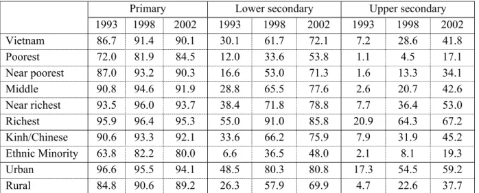
Table 3.4: Net enrollment rates (%)

Primary Lower secondary Upper secondary

1993 1998 2002 1993 1998 2002 1993 1998 2002 Vietnam 86.7 91.4 90.1 30.1 61.7 72.1 7.2 28.6 41.8 Poorest 72.0 81.9 84.5 12.0 33.6 53.8 1.1 4.5 17.1 Near poorest 87.0 93.2 90.3 16.6 53.0 71.3 1.6 13.3 34.1 Middle 90.8 94.6 91.9 28.8 65.5 77.6 2.6 20.7 42.6 Near richest 93.5 96.0 93.7 38.4 71.8 78.8 7.7 36.4 53.0 Richest 95.9 96.4 95.3 55.0 91.0 85.8 20.9 64.3 67.2 Kinh/Chinese 90.6 93.3 92.1 33.6 66.2 75.9 7.9 31.9 45.2 Ethnic Minority 63.8 82.2 80.0 6.6 36.5 48.0 2.1 8.1 19.3 Urban 96.6 95.5 94.1 48.5 80.3 80.8 17.3 54.5 59.2 Rural 84.8 90.6 89.2 26.3 57.9 69.9 4.7 22.6 37.7

Note: Those who reported being in school and having only completed the level immediately below are

considered enrolled at each level. At the secondary level, enrolment might thus include those who are in technical or vocational schools. However, the proportion of children of secondary school age who are in vocational or technical schools is very small (in 1998 it was estimated at 0.05 per cent for lower secondary and 1.69 per cent for upper secondary). Those figures are estimated using data from the VLSS 1992/93, VLSS 1997/98, and VLSS 2001/02

Source: World Bank et al. (2003)

Although a sharp decline in enrolment rate at all levels of education occurred from 1986 to 1991, this trend did not last long. Since 1992, the enrolment rate has began to increase at all school levels by all measurements. The net enrolment rate (NER) for children at the age of primary education increased from 86.7% in 1993 to 91.4% in 1998 and slightly reduced to 90.1% in 2002. For children at the age of lower secondary education, the net enrolment rates also increased drastically from 30.1% in 1993 to 61.7% in 1998 and further increased to 72.1% in 2002 (Table 3.4)11. Note that the pace of changes has been much slower during 1998-2002 than

11_{The gross enrolment rate is the number of children enrolled in a level of education, regardless of age, as}

(26)

that during 1993-98. This means that the national targets of the NERs of 97% and 80% for children at the age of primary and lower secondary education by 2005 respectively, may be hard to be achieved. Moreover, in terms of NER, the gaps between Kinh/Chinese majority and ethnic minorities and between rural and urban areas, though declining, are still significant.

Together with the enrolment rate, at the beginning of each school year, the Ministry of Education and Training (MOET) issues a report in which the dropout rate is also presented. According to this report, a child is viewed as dropout if he/she did not continue his/her schooling given he/she had enrolled at least part of the last schooling year. This definition is sometimes criticized as inaccurate since it does not count those who do not continue to enrol in the school after having finished a given grade. This leads to the underestimation of school dropout situation in Vietnam12.

Slightly different from the official definition used by the MOET, in this study, a child is called to be a dropout if he/she has not completely enrolled in schools in the 12 month prior to the survey, given he/she used to enrol in school sometime before. This definition provides a more precise picture of dropout situation in Vietnam, although it still suffers from some shortcomings such as inclusion of small number of children who had to postpone their education due to specific reasons and intended to continue their education in the next coming year.

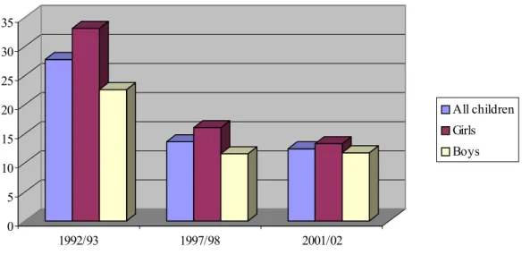
As indicated by Figure 3.1, the school dropout rate dropped considerably, from as high as 27.7% in 1993 to as 12.4% in 2002. This reduction occurred largely during the period 1993 – 1998, which witnessed a booming of Vietnam’s economy. In this period the dropout rate has reduced by 14.0 percentage points. However, in the following period from 1998 to 2002, the proportion of children dropped out of school has just reduced by 1.3 percentage points. Thus, the pattern of

enrolled in a level of education who are of official school age for that level, as a percentage of the population of official school age for that level.

12_{For example, in the schooling year 1999/2000, the number of pupils enrolling in the primary schools}

was 10,063,025. Of which the promotion rate, calculating by the ratio of those who satisfy qualifications to promote to higher grade over those enrolling in the beginning of the schooling year, was 92.5%, the repeat rate is 2.8% and the dropout rate is 4.7%. In the schooling year 2000/01, the promotion rate was 94.0%, the repeat rate is 2.3% and the dropout rate is 3.7%. In 2001/02, the promotion rate was 95.1%, the repeat rate is 1.8% and the dropout rate is 3.1%. This means that the dropouts are those who did enroll

(27)

changes in dropout rate (and also in NER) seems to be in line with the pattern of poverty reduction in Vietnam during 1993-200213.

The decline in school dropout rate was much pronounced for girls than for boys. The gap between boys’ and girls’ dropout rates narrowed from 10.4 percentage points in 1993 to 4.6 percentage points in 1998 and further to only 1.6 percentage points in 2002(Figure 3.1).

Figure 3.1: Overall dropout rates in 1993, 1998 and 2002

0 5 10 15 20 25 30 35 1992/93 1997/98 2001/02 All children Girls Boys

Source: Authors’ calculation using VLSS 1992/93, VLSS 1997/98 and VLSS 2001/02

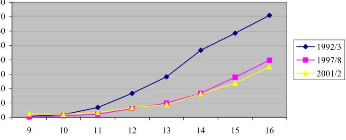
The school dropout rate varies considerably across various age groups. Figure 3.2 shows that the age that saw the largest withdrawal from school increased from around 12 years old in 1993 to 14 years old in 1998 and 2002. In 1993, from the age of 12, the proportion of children reported that they did not enrol in school in 12 months prior to the survey steeply increased from 16.7% for the children of 12 years old to 28.2% for children of 13 years old, 46.7% for children of 14 years old, 58.6% for children of 15 years old, and 71.0% for children of 16 years old. The situation improved rather well in 1998 and 2002. Only more than 6% of children of 12 years old reported not enrolling in school in the 12 months prior to the surveys. This figure slightly increased to 9.9% in 1998 and 9.0% in 2002 for 13-year-old children. From the age of 14, the number of those who did not enrol in school fairly rapidly increased from more than 16% for

(28)

year-old children to 39.3% and 35.2% for children of 16 years old in 1998 and 2002, respectively. This implies that the dropout situation did really improve during the last ten year, although the pace of changes again had slowed down during 1998-2002.

Figure 3.2: Dropout rates in 1993, 1998 and 2002, by age

0 10 20 30 40 50 60 70 80 9 10 11 12 13 14 15 16 1992/3 1997/8 2001/2

Girls usually dropped out earlier than their male counterparts, although there is some sign of improvement in the recent years (Figure 3.3). In 1993, 23.6% of girls dropped out at the age of 12 while only 9.1% of boys dropped out at the same age. At the age of 16, 79.0% of girls dropped out and only 63.7% of boys did. In 1998, the number of girls dropped out of school at the age of 12 reduced significantly to 8.4%, but this figure was still twice higher than that of boys. Similarly, by the age of 16, the proportion of girls dropped out is still 11.2 percentage points higher than that of boys. In 2002, the situation had slightly changed. For children aged 9, 10 and 11, the percentage of those who did not enrol in school in the 12 months prior to the survey was slightly higher than that in 1993 and 1998, although the proportions of female and male dropped out of schools in 2002 generally were lower than that in 1993 and 1998. Moreover, the gap in dropout between girls and boys narrowed rather impressively. By the age of 16, the gap between girls’ and boys’ dropout rates was only 4.3 percentage points.

(29)

Figure 3.3: Dropout rates of girls and boys in 1993, 1998, and 2002, by age 0 10 20 30 40 50 60 70 80 90 9 10 11 12 13 14 15 16 Girls 1992/93 Boys 1992/93 Girls 1997/98 Boys 1997/98 Girls 2001/02 Boys 2001/02

Figure 3.4 displays the dropout distribution among the education cycles in 1993, 1998 and 2002. Most of dropout children selected to withdraw from education system at the primary education. This means that a considerable number of the children who dropped out of schools had only primary education or lower. In 1993, 55.3% of those who dropped out left school after finishing primary education or some classes in the primary cycle. This figure increases to 60.1% in 1998, and then reduces to 50.9% in 2002. Interestingly, dropout boys are more likely to leave schools after finishing the primary cycle or some classes in this cycle than girls do. This pattern can be seen in 1993, 1998 and 2002.

(30)

Figure 3.4: The dropout distribution among education cycles in 1993, 1998, and 2002 0% 20% 40% 60% 80% 100% All c hildr en 9 2/3 Boys 92/3 Girls 92/3 All ch ildren 97/8 Boys 97/8 Girls 97/8 All ch ildren 01/2 Boy s 01/2 Girls 01/2 Upper secondary Lower secondary Primary First class

Figure 3.5 displays the school dropout rates across Vietnam’s seven regions. Due to the regional specific characteristics and development, the dropout rates and the patterns of their changes are quite different from region to region. In 1993, the Central High Land, and Southern Central Cost regions had the lowest dropout rates, while Mekong River Delta and Northern Mountain regions had the highest dropout rates. In 2002, the lowest dropout rates could be observed in the Northern and Southern Central Coasts regions, while the highest rates were of Mekong River Delta and South East regions. The dropout rates declined in all regions from 1993 to 2002, but they slightly increased in some regions during 1998 - 2002. Surprisingly, the region recorded the highest achievement in reducing the dropout rate over the last ten years is the Northern Mountain, one of the poorest regions. Meantime, the Central Highland, another poorest region, was much less successful despite a sharp decline in the dropout rate between 1992/93 and 1997/9814.

14_{Some economists have explained this phenomenon by presenting that during 1997/98 – 2001/02, there}

(31)

Figure 3.5: Dropout rates in 1993, 1998 and 2002, by region Red Ri ver Northe rn Mo untai n North ern C entra l Southe rn C entral Cent ral H ighlan d South East Meko ng D elta 2001/2 199 7/8 19 92/₃ 0 5 10 15 20 25 30 35 2001/2 1997/8 1992/3

3.3. Causes of schooling dropout – a qualitative analysis

The theoretical framework and international evidences presented in Section 2 suggest that there are several factors, which may explain why children dropped out of schools. These factors can be ranged from family’s economic situation and characteristics to those that are out of the household and child's immediate controls.

It is important first to look at the schooling dropout rates across household expenditures quintiles. Figure 3.6 shows that the dropout rate declined significantly for all expenditure

quintiles over the period 1993-2002. For example, the dropout rate of children living in 20% poorest households declined from 33.5% in 1993 to 19.6% in 1998 and further to 15.3% in 2002. However, there remains a wide gap in dropout rates across expenditures quintiles, especially between 20% richest and 20% poorest households. Moreover, in the second spell from 1998 to 2002, the dropout rate surprisingly increased from 10.5% to 11.6% for those children living in the households belonging to the 4th expenditure quintiles and from 3.6% to 7.0% for those children living in the 20% richest households. This implies that during the last 5 years, the dropout rate may be less responsive to total household expenditure.

(32)

Figure 3.6: School dropout rate across expenditure quintiles 0 5 10 15 20 25 30 35 40 Lowest (1st) 2nd 3rd 4th Richest (5th) 1992/3 1997/8 2001/2

A decline in responsiveness of dropout rate to total household expenditure may be also reflected in the pattern of household expenditures on education (or direct cost of schooling). During 1993

– 2002, the cost of schooling for a child increased by 126.3% while per capital expenditure increased just by 67.0% (Figure 3.7). Interestingly, the dropout rate felt rather fast during 1993-1998 when the cost of schooling increased quickly, meaning a rather weak association between the dropout rate and cost of schooling. Figure 3.7 also shows that the cost of schooling has increased as the child aged. For those children at the age of 9, the cost of schooling is about 3 times lower than that of children at the age of 16. This also helped to explain why the dropout rate is much higher among children at the higher ages. Higher the age of the child, higher the opportunity cost of attending school would be.

(33)

Figure 3.7: Cost of schooling per student in 1993, 1998 and 2002, by age 0 100 200 300 400 500 600 700 800 900 9 10 11 12 13 14 15 16 1992/3 1997/8 2001/2

The cost of schooling per student is also very different from region to region (Table 3.5). Of all the regions, the average cost of schooling in the poorest region, Northern Mountain region, is lowest and the cost of the richest region, the South East region, is highest. This seems to be not corresponding to the change in dropout rates in these regions during 1993-2002 (see Section 3.2). While the cost of schooling could be important factor for explaining dropout situation in general, it alone hardly can explain the difference among the regions in terms of dropout rate. Indeed, the correlation coefficients by region between dropout rate and share of household expenditures on education in total expenditure are –0.25 in 1993, 0.13 in 1998, and –0.60 in 2002.

Table 3.5: Direct cost of schooling per student by region (1994-prices; ‘000 VND)

1993 1998 2002

Region Cost of schoolCost of school

% change compared to 1993 Cost of school % change compared to 1993 Red River 93.41 288.05 208.37% 281.31 201.16% Northern Mountain 57.32 132.73 131.56% 155.9 171.98% Northern Central 68.27 209.49 206.86% 220.52 223.01% Southern Central 204.36 388.15 89.93% 278.17 36.12% Central Highland 110.19 190.46 72.85% 246.62 123.81% South East 211.6 547.65 158.81% 403.87 90.86% Mekong Delta 172.07 333.42 93.77% 216.6 25.88% Whole country 95.35 269.33 182.46% 215.76 126.28%

Can Vietnam Achieve One of its Millennium Development Goals? An analysis of schooling dropouts of children

T

HE

W

ILLIAM

D

AVIDSON

I

NSTITUTE