Research Division
Federal Reserve Bank of St. Louis
Working Paper Series
Saving and Growth under Borrowing Constraints: --
Explaining the “High Saving Rate” Puzzle
Yi Wen
Working Paper 2009-045C
http://research.stlouisfed.org/wp/2009/2009-045.pdf
September 2009
Revised June 2010
FEDERAL RESERVE BANK OF ST. LOUIS
Research Division
P.O. Box 442
St. Louis, MO 63166
______________________________________________________________________________________ The views expressed are those of the individual authors and do not necessarily reflect official positions of the Federal Reserve Bank of St. Louis, the Federal Reserve System, or the Board of Governors.
Federal Reserve Bank of St. Louis Working Papers are preliminary materials circulated to stimulate discussion and critical comment. References in publications to Federal Reserve Bank of St. Louis Working Papers (other than an acknowledgment that the writer has had access to unpublished material) should be cleared with the author or authors.
Saving and Growth under Borrowing Constraints:
Explaining the "High Saving Rate" Puzzle
Yi Wen
Federal Reserve Bank of St. Louis &
Tsinghua University (First Version: September 2009)
(This Version: May 2010)
Abstract
This paper shows that uninsured risk and borrowing constraints can make an individual’s marginal propensity to consume negatively dependent on his/her permanent income. Therefore, higher income growth can lead to higher saving rates without requiring (or causing) high interest rates — in sharp contrast to implications of the permanent income hypothesis. For example, the model predicts that household saving ratio can rise from5%to25%when the annual rate of income growth increases from1%to10%, despite a …xed1%real deposit rate. The predictions are consistent with the experience of emerging economies, such as Japan (in the 1950-70s) and China (over the past 30 years).
Keywords: Permanent Income Hypothesis, Borrowing Constraints, High Saving Rate Puzzle, Chinese Economy, Growth and Development, Global Imbalance, Global Savings Glut.
JEL Codes: D91, E21, O16.
I thank Costas Azariadis, Kaiji Chen, Qing Liu, Dennis Tao Yang, Xiaodong Zhu, and especially Charles Yuji Horioka, as well as seminar participants at the Federal Reserve Bank of St. Louis, Tsinghua University (Beijing campus and Taiwan campus), and Osaka University for comments. I also thank Jessy Zhengjie Qian, Alex Segura, and Qiong Zhang for providing data and research assistance, and Judy Ahlers for editorial assistance. The views expressed in this paper do not re‡ect the o¢ cial positions of the Federal Reserve Bank of St. Louis, and the usual disclaimer applies. Correspondence: Yi Wen, Research Department, Federal Reserve Bank of St. Louis, P.O. Box 442, St. Louis, MO, 63166. Phone: 314-444-8559. Fax: 314-444-8731. Email: [email protected].
1
Introduction
The canonical permanent income hypothesis (PIH)1predicts that forward-looking consumers should
save less when income growth is high because they expect to be richer in the future than they are today. Accordingly, saving rates should be lower in fast-growing countries than in slow-growing countries.
This prediction has led to the well-known "high saving rate" puzzle for fast-developing economies (such as Japan in the 1950-70s and China in the past 30 years). Much e¤ort has been devoted to resolving this puzzle without reaching a consensus. For example, Horioka (1985, 1990) provides a comprehensive list of various life-cycle factors that may contribute to Japan’s high saving rate, including precautionary saving, housing …nance, and income growth. However, careful analysis of the implications of the life-cycle hypothesis leads Hayashi (1986) to reject it as a plausible theory of Japan’s saving behavior. In particular, Hayashi concludes that high income growth cannot explain Japan’s high saving rate because the life-cycle hypothesis depends on heterogeneous cohort e¤ects to generate the positive link between growth and aggregate saving, but such cohort e¤ects are inconsistent with Japanese data.
Yet, empirical evidence suggests that saving and growth are strongly positively correlated, and the positive correlation holds largely because high growth leads to high saving, not vice versa.2 Nonetheless, most theoretical e¤ort has been devoted to understanding the growth-to-saving causal-ity in a life-cycle framework, because it is thought that this fact is inconsistent with optimal con-sumption behavior in an in…nite-horizon permanent-income framework.
A leading alternative view is that the PIH fails because it is based on, among other things, the assumption of exogenous rates of returns to …nancial assets (i.e., the real interest rate). In a production economy with productive assets (such as capital), the real rates of return are determined by the marginal products of such assets. When asset returns are so determined, they will respond to changes in productivity growth, which is the fundamental source of changes in permanent income. A permanent increase in total factor productivity (TFP) raises the rate of return to capital, so investment demand will increase, resulting in a higher equilibrium saving rate through a higher real interest rate. Consequently, in contrast to the prediction of the PIH, standard general-equilibrium growth theory suggests that household saving may increase rather than decrease in response to a higher permanent income (as implied by the analysis of Chen, Imrohoroglu, and Imrohoroglu, 2006).
1
Friedman (1957).
2
However, fast-growing economies tend to have not only high saving rates, but also low and essentially …xed interest rates. For example, in Japan in the 1950-70s, the household saving rate was as high as23%, while the real 3-month time deposit rate was negative for the entire period.3 Similarly, in China over the past 30 years, the average personal saving rate has been about 25%, yet the real 1-year deposit rate has been below zero.4 Hence, the puzzle is not just why high growth can lead to high saving (or vice versa), but also why a high saving rate is possible when the interest rate is so low.5
This paper argues that su¢ ciently large uninsured uncertainty and borrowing constraints may hold the key for understanding the triple phenomena of "high saving, high growth, and low in-terest rate" for fast-growing countries. That households are subject to borrowing constraints and uninsured idiosyncratic risk has been extensively documented and studied in the literature for devel-oped countries (see, e.g., Aiyagari, 1994, and Gross and Souleles, 2002, and the references therein). Agents in developing countries are typically far more borrowing constrained and far less insured for idiosyncratic shocks than those in developed countries, because of the lack of social safety nets and under-developed …nancial and insurance markets. Skinner (1986) presents empirical evidence that income uncertainty is a key factor determining households’ precautionary savings in developing countries.
Precautionary saving under borrowing constraints can completely alter the relationship between permanent income and consumption by making the marginal propensity to save a positive function of permanent labor income, so that faster income growth generates an increased propensity to save regardless of interest rates. As a result, high growth can lead to high saving without requiring or causing high interest rates. In other words, even if the deposit rate is …xed at zero, household saving may still be excessively high and respond positively to income growth.6 For the same reason, borrowing constraints can support a large spread between the deposit rate and the rate of return to capital in general equilibrium. Consequently, fast-growing economies may appear to have undiminished high rates of return to capital despite a high investment-to-output ratio.7
3An extensive literature argues that the Japanese government repressed interest rates in that period to promote
investment and stimulate growth (see, e.g., Horiuchi, 1984; Patrick and Rosovsky, 1976). Dekle (1993) and Homer and Sylla (2005) also note that real interest rates were never particularly high in Japan, but were higher in the low-saving, low-growth 1920s than in the high-saving, high-growth 1960s. Although the rates of return on corporate equities were very high in Japan during that period, households’ share of equities was quite low (see, e.g., Horioka, 1990).
4
The fact that the real interest rates in China have been kept very low since the economic reform is well known (see, e.g., Zou and Sun, 1996). Because households’ access to …nancial markets and investment opportunities are typically very limited and stockmarket is extremely risky, deposits have been the major means of saving and the most important contributor to China’s aggregate saving ratio despite the low interest rates (see, e.g., Kraay, 2000).
5As a reference point, in the standard neoclassical growth model presented in the next section, when the rate of
income growth reaches10%per year, the aggregate saving rate can reach about20%. However, to support this high
saving rate, the real interest rate must be about15%.
6This would not be the case without uninsured risk and borrowing constraints. In a standard growth model, the
saving rate would decrease with income growth if the interest rate were constant, as predicted by the PIH.
7For example, the real rate of return to capital has been over20%a year for the past 30 years in China, and it
The main intuition is that uninsured risk and borrowing constraints induce precautionary sav-ings, even if the interest rate is low (imagine why rational agents hold inventories despite negative rates of return — because inventories yield a liquidity premium). If the degree of uncertainty re-mains constant relative to the income trend, agents would want to maintain a stable stock of savings relative to trend because of the need for self-insurance; namely, they prefer to maintain a constant bu¤er stock to income ratio along a balanced growth path. Since income is a ‡ow, when it grows, a larger portion of the ‡ow must be devoted to the accumulation of the stock ("investment"); oth-erwise, the stock-to-‡ow ratio would decline sharply, which would hinder the bu¤er-stock function of savings and reduce the extent of self-insurance. Thus, the saving rate should rise with income growth. In other words, the e¤ective rate of return to saving is the real interest rate compounded by a liquidity premium. When the growth rate of income rises, the liquidity premium increases if the saving stock falls relative to the income trend. A higher liquidity premium thus induces a higher saving rate.8 Therefore, the predictions of the canonical PIH are completely altered: High growth leads to high saving, even with low (and …xed) interest rates.
These arguments are formalized in this paper in an in…nite-horizon neoclassical growth model (with or without capital), where long-run income growth is driven by exogenous TFP changes and households face uninsured idiosyncratic shocks and are borrowing constrained. To facilitate the analysis, some simplifying assumptions are necessary to make the model analytically tractable. When markets are incomplete and agents are heterogeneous, analytical tractability not only reduces the computational costs of comparative analysis, but also makes the mechanisms transparent.9 The key simplifying assumptions include (i) The utility function is quasi-linear.10 (ii) Labor supply decisions of all households must be made before observing their idiosyncratic shocks in each period. The second assumption implies that a spot labor market does not always exist and it ensures the bu¤er-stock function of savings — otherwise, current wage income can be adjusted immediately to fully bu¤er any shocks to income or preferences within the same period.11 In addition, we need to place the idiosyncratic shocks on preferences or gross wealth instead of labor earnings.12 Under these assumptions, the optimal growth model with borrowing constraints has closed-form solutions
8However, to keep the stock-to-‡ow ratio exactly constant as income grows faster is very costly — the opportunity
cost of not consuming the rising income increases with income growth. Hence, although the saving rate may increase, it may not increase enough to achieve the original stock-to-‡ow ratio. So in a new steady state with a higher growth rate, the optimal stock-to-‡ow ratio is lower than before despite a higher saving rate. This means that the liquidity premium increases by just enough to balance the marginal costs of saving and the marginal bene…ts of saving.
9
Given that our results are in sharp contrast to conventional wisdom and may appear to be counterintuitive, closed-form solutions are preferred to numerical results.
1 0Although this assumption implies an in…nitely elastic labor supply, it is nonetheless realistic for developing
economies such as China — the large rural population in provides an abundant supply of labor.
1 1This assumption is not needed if labor supply is inelastic or the leisure function is nonlinear, but then the model
becomes analytically intractable.
1 2Even with quasi-linear preferences, the model is not analytically tractable if the idiosyncratic shocks come directly
from labor income (see, e.g., Imrohoroglu, 1989; Zeldes, 1989; Deaton, 1991; Carroll, 2001; Aiyagari, 1994; Krusell and Smith, 1998).
for individuals’optimal consumption and saving plans. Aggregating by the law of large numbers, the general equilibrium of the model can be solved by standard methods in the representative-agent real business cycle (RBC) literature, and dynamic impulse responses of aggregate savings to both transitory and permanent changes in the growth rate of TFP (the source of permanent income) can be easily analyzed.
An important property of the model is that it reduces to a representative-agent, frictionless neoclassical growth model with aggregate uncertainty when the distribution of idiosyncratic shocks becomes degenerate. This property makes the model easily comparable to standard growth models by changing the parameter values that control the strength of precautionary saving and borrowing constraints.13
This paper is closely related to those by Jappelli and Pagano (1994), Carroll, Overland, and Weil (2000), and Chen, Imrohoroglu, and Imrohoroglu (2006). Jappelli and Pagano (1994) study the relationships between saving and growth under borrowing constraints in a simple overlapping-generations model. They show that borrowing constraints can enhance the positive e¤ect of growth on saving. However, as pointed out by Modigliani (1970), Hayashi (1986), and many others, in life-cycle models the positive e¤ect of growth on saving is largely the result of aggregation. To the extent that the economy is growing, workers’ savings will increase relative to retirees’ dissavings, thus, measured aggregate savings will increase. In contrast, this paper studies the issue in an in…nite-horizon growth model in which the positive growth-to-saving e¤ect originates from a di¤erent mechanism. That borrowing constraints can increase precautionary saving at a given level of income growth is well known, but whether borrowing constraints can also generate a positive causal e¤ect of growth on saving in an in…nite-horizon permanent-income framework is unclear. In this regards, this paper complements the analysis of Jappelli and Pagano (1994).14
Alternatively, Carroll, Overland, and Weil (2000) use an in…nite-horizon endogenous-growth model with habit formation to explain the positive e¤ect of growth on saving. Habit formation can generate a positive growth-to-saving e¤ect because it makes consumption "sticky"; consequently, an increase in permanent income will raise saving …rst before it has a full impact on consumption. However, in this endogenous-growth model, high growth necessarily implies a high real interest rate, which is inconsistent with the experience of Japan and China. Also, Chamon and Prasad’s (2009) empirical analysis based on Chinese household data does not support habit formation as a plausible explanation for China’s high household saving rates.
1 3
The solution techniques applied in this paper are similar to those in Wen (2009).
1 4
The idea that borrowing constraints can lead to excessive saving and can be a possible source of failures of the PIH is hardly new. For example, see Zeldes (1989), Imrohoroglu (1989), Deaton (1991), Carroll (1992, 1997), Aiyagari (1994), and Huggett (1997), among many others. However, the implications of borrowing constraints for the aggregate relationship between saving and growth have not previously been examined in a rigorous in…nite-horizon growth model, to the best of my knowledge. In addition, none of the above-cited works provides closed-form saving functions under borrowing constraints in an in…nite-horizon model as is done in this paper.
More recently, Chen, Imrohoroglu, and Imrohoroglu (2006) use a standard neoclassical growth model to o¤er a quantitative account of the time path of Japan’s saving rate in the postwar period. Their simulations, based on actual time-series data and the assumption of perfect foresight, reveal that stochastic TFP growth is the main force driving Japan’s saving rate. But their model also requires high interest rates to induce high saving rates and they do not address the low interest rate issue.
This paper also has implications for global imbalances and global savings glut. If fast-growing economies opt to save excessively more because of higher income growth and less developed …nancial markets, it is then natural to observe out‡ows of savings from these economies toward developed countries where the interest rates are high, and in‡ows of foreign direct investment (FDI) from developed countries toward these emerging economies with faster TFP growth and high marginal products of …xed capital. In this regard, this paper is also closely related to the work of Caballero, Farhi, and Gourinchas (2008), Ju and Wei (2006), Mendoza, Quadrini, and Rios-Rull (2009), and Song, Storesletten, and Zilibotti (2009). These papers all emphasize ine¢ cient …nancial system in emerging economies as the key contributing factor to their …nancial capital out‡ows. However, none of these papers aims at explaining why high growth can lead to high saving despite low interest rates.15
The rest of the paper is organized as follows. Section 2 presents the model and derives closed-form decision rules for household consumption and saving. Section 3 studies the general-equilibrium e¤ects of growth and borrowing constraints on saving behavior along balanced growth paths. Sec-tion 4 studies the transiSec-tional and short-run dynamics of the aggregate saving rate. SecSec-tion 5 reconsiders the growth-to-saving e¤ects in a counterfactual experiment with a …xed deposit rate. Section 6 shows that the predictions of the model are consistent with the experience of China and Japan during their high-growth periods. Section 7 concludes the paper with remarks for fu-ture research. The robustness of the results for more general utility functions is analyzed in the Appendix.
2
The Model
2.1 Households
There are a continuum of households indexed by i 2 [0;1]. Taking as given the market real interest rate rt, real wage Wt, and pro…t income Vt from …rms, household i chooses sequences of consumption Ct(i), savings St+1(i), and labor supply Nt(i) to maximize expected lifetime utility,
EP1t=0 tflogCt(i) aNt(i)g, subject to the budget constraintCt(i) +St+1(i) ["t(i) + ]Xt(i),
1 5
Song, Storesletten, and Zilibotti (2009) explain China’s high growth rate while taking as given its high saving rate. This paper complements their analysis by o¤ering an explanation of China’s high saving rate.
whereXt(i) [(1 +rt)St(i) +WtNt(i) +Vt]denotes householdi’s wealth income or cash in hand,16 which includes initial wealth,(1 +r)St(i), labor income,WtNt(i), and any lump-sum transfers such as …rms’pro…t incomeVt. Households are borrowing constrained, so we imposeSt+1(i) 0in each
period following the standard literature. The log form of the utility function ensures the existence of a balanced growth path.17
Note that cash in hand is subject to a multiplicative idiosyncratic shock, +"t(i), where 2(0;1) is a constant multiplier, and "t(i) is i.i.d. with mean E"(i) = 1 . This implies that fraction of the wealth income is never subject to idiosyncratic shocks. The expected value of the shock is normalized toE"(i) = 1 so that the average value of +"(i)equals1; thus, idiosyncratic shocks do not cause distortions to the budget constraint on average or at the aggregate level.18 The model reduces to a representative-agent model either if = 1 or the variance of"t(i) becomes zero.19
An interpretation of the wealth-income shock is disaster risk: Nature randomly destroys a portion of household wealth in each period. Since disaster risk is not fully self-insurable, the model can be easily calibrated to match the wealth inequality in the data if is small enough, even though "(i) is i.i.d.20 This type of shocks helps to capture the severity of idiosyncratic risk in developing countries (such as tra¢ c and various types of accidents, natural and social-political disasters, robbery, unemployment, illness, erratic changes in the value of wealth, and so on). However, with respect to the main results of the paper, this assumption is innocuous — it is mainly a technical device to obtain closed-form solutions because it is well known that with CRRA utility functions, an in…nite-horizon consumption model with borrowing constraints is not analytically tractable if the idiosyncratic risk derives directly and solely from labor income. The model is also tractable if the idiosyncratic shocks are placed on preferences instead of cash in hand (see Wen, 2009) and the main results of the paper remain intact, which is reassuring since it suggests that the key mechanisms uncovered in this paper are robust to the assumptions of the sources of idiosyncratic risks.21
1 6
In this paper, "wealth income" and "cash in hand" are used interchangeably.
1 7The Appendix shows that the qualitative results do not hinge on the log form of the utility function.
1 8
The multiplicative assumption of individual wealth-income shocks implies that the degree of risk remains constant relative to the balanced growth path and does not diminish with growth — namely, wealth inequality remains stable as the economy grows. This implication is consistent with empirical evidence (see, e.g., Wol¤, 1998). The same assumption is made in the literature of incomplete markets where idiosyncratic earning (or labor productivity) shocks are multiplicative to the real wage, suggesting that the degree of income uncertainty does not diminish as the real wage grows over time (see, e.g., Aiyagari, 1994). Still, without economic analysis, such assumptions do not indicate whether the saving rate should increase or decrease with growth. On the other hand, it is unrealistic to assume that the idiosyncratic shocks are additive to wealth or income, which would imply that as wealth or income grow over time the signi…cance of such shocks diminishes to zero.
1 9
When !1, the distribution of"(i)becomes a degenerate delta function with a unit mass centered at0.
2 0Aiyagari (1994) and Krusell and Smith (1998) show that idiosyncratic risk stemming from labor income alone
cannot generate enough inequality across households to explain the wealth distribution in the United States because such shocks are almost fully self-insurable unless they are highly persistent.
2 1The point made in this paper is more general than it may appear under the speci…c assumptions of the stylized
model, since (i) the source of the uninsured idiosyncratic risk is irrelevant, (ii) agents always need to accumulate a bu¤er stock of savings, and (iii) they want to maintain a stable stock-to-‡ow ratio on the balanced growth path.
The information structure and sequence of events are as follows. Within each time period t, there are two subperiods. All aggregate shocks are realized in the beginning of the …rst subpe-riod but the idiosyncratic shocks are realized only in the second subpesubpe-riod. In the …rst subpesubpe-riod, households choose labor supply Nt(i) after observing period-t aggregate shocks but without ob-serving the idiosyncratic wealth-income shocks. In the second subperiod, the idiosyncratic shocks
"t(i) are realized and households then choose consumption and savings to maximize expected life-time utilities.22 Without loss of generality, assume a= 1. The population is constant over time. Idiosyncratic shocks are assumed to be orthogonal to any aggregate shocks.
2.2 Firms
There is a unit mass of identical …rms producing output (Yt) according to the technology, Yt =
Kt (ZtNt)1 , where Zt denotes a nonstationary process of labor-augmenting technology, which grows over time according to the process Zt= (1 +gt)Zt 1. The capital stock (K) is accumulated
according toKt+1= (1 )Kt+It, whereI is investment per …rm. The stochastic growth rategt has mean g 0 and follows the law of motion:
gt g= g(gt 1 g) + t; (1) where g 0measures the persistence of the aggregate growth shock and the innovation tis i.i.d with zero mean. Wheng= 0 and g= 0, the dynamic e¤ects ofZtare identical to a random-walk technology shock without drift. With a little abuse of language, we use the terms "technology" and "TFP" interchangeably, although Zt re‡ects labor-augmenting technology. We assume the existence of capital rental markets, as in Aiyagari (1994). Firms behave competitively; hence, the real factor prices are determined by their respective marginal products: Wt = (1 )NYtt and
rt+ = KYtt, wherer+ is the user’s cost of capital with capital depreciation 2[0;1]. Because of constant returns to scale, the pro…t income is zero, Vt= 0.
2.3 Transformation
The model is not stationary in the level but is stationary in the growth rate. In the absence of aggregate uncertainty (i.e.,gt=g for all t), the aggregate economy has a unique balanced growth path along which the real interest rate and aggregate hours worked, N R N(i)di, are constant, and the other aggregate variables, such as Ct
R
C(i)di, St+1
R
S(i)di, Kt+1, Yt, and Wt all Therefore, the liquidity premium of the bu¤er stock must rise whenever the stock-to-‡ow ratio declines, which will trigger a higher saving rate.
2 2This timing structure implies that households may not be able to fully self-insure against idiosyncratic risk by
grow at the same rate g. Hence, to solve for the competitive equilibrium, we can transform the model into a stationary one by scaling it down by the growth factor (1 +g) t. Using lowercase letters to denote the transformed variables (e.g., yt (1+Ytg)t),23 the production function and the
real factor prices become
yt=kt (ztNt)1 (2) wt= (1 ) yt Nt (3) rt+ = yt kt ; (4)
respectively. Other relationships such as the capital accumulation equation can be transformed analogously.
After the transformation, household i’s maximization problem can be written more compactly as max fc;s0gE0 ( max fNg ~ E0 ( 1 X t=0 t[logc t(i) Nt(i)] )) (5) subject to ct(i) + (1 +g)st+1(i) ["t(i) + ]xt(i) (6) st+1(i) 0; (7) where xt(i) (1 +rt)st(i) +wtNt(i) +vt (8) de…nes the transformed cash in hand net of the idiosyncratic multiplier, and the expectation oper-ator E~t in the objective function denotes expectations conditional on the information set of time
t excluding "t(i), and the operator Et denotes expectations based on the full information set in periodtincluding"t(i). These notations re‡ect the information and timing structure of the model. The idiosyncratic i.i.d. shock has support "2[0; "max], cumulative distribution function F("), and
the unconditional mean R"dF = 1 . The mean requirement implies "max>1 .
2.3.1 Decision Rules
Denoting f (i); (i)g as the Lagrangian multipliers for constraints (6) and (7), respectively, the …rst-order conditions for fc(i); N(i); s(i)g are given, respectively, by
1
c(i) = (i) (9)
2 3To obtain the equilibrium path of the untransformed variables, we can apply the inverse transformation, such as
Yt= (1 +g)tyt and YYt
t 1 = (1 +g)
yt
1 =wtE~tf["t(i) + ] t(i)g=wt
Z
["t(i) + ] t(i)dF(") (10)
(1 +g) t(i) = Etf(1 +rt+1) ["t+1(i) + ] t+1(i)g+ t(i); (11) where equation (10) re‡ects the fact that labor supplyNt(i)is determined before "t(i) (and hence the value of t(i)) is realized. By the law of iterated expectations and the orthogonality assumption of aggregate and idiosyncratic shocks, equation (11) can be written as
(1 +g) t(i) = Et (1 +rt+1) Z ["t+1(i) + ] t+1(i)dF(") + t(i) = Et 1 +rt+1 wt+1 + t(i); (12) where the …rst equality applies the law of iterated expectations and the orthogonality assumption, and the second equality uses equation (10).
The optimal consumption and saving plans of each individual are characterized by a cuto¤ strategy, where the cuto¤ ("t) is related to the realization of the idiosyncratic shock. We assume interior solutions for labor supply and use a guess-and-verify strategy to derive the decision rules. A key step in the analysis is to show that the cuto¤"t, as well as the optimal cash in hand xt, are independent ofi.
Proposition 1 The decision rules for consumption, saving, and cash in hand for any household i
are given by ct(i) = min "t(i) + "t + ;1 ["t + ]xt (13) (1 +g)st+1(i) = max "t(i) "t "t+ ;0 ["t + ]xt (14) xt= (1 +rt)st(i) +wNt(i) +vt=wtR("t) 1 "t + ; (15)
where the cuto¤ "t is determined by the equation
1 +g wt = Et 1 +rt+1 wt+1 R("t); (16)
in which the implicit functionR( ) is given by
R("t) + "Z "<"t "tdF(") + Z " "t "dF(") # >1: (17)
Proof. In anticipation that the cuto¤ is independent ofi, consider two possible cases:
Case A. "t(i) "t. In this case, the e¤ective cash in hand is high. To smooth consumption, it is optimal to save to prevent possible borrowing constraints in the future when cash in hand may be low. So st+1(i) 0, t(i) = 0, and the shadow value of good t(i) = Et(1+1+gr)tw+1t+1. Equation (9) implies that consumption is given byct(i) =
h
Et(1+1+gr)tw+1t+1
i 1
. The budget constraint (6) then implies(1 +g)st+1(i) = ["t(i) + ]xt
h
Et(1+1+gr)tw+1t+1
i 1
. The requirementst+1(i) 0then implies
"t(i) + 1 xt Et 1 +rt+1 (1 +g)wt+1 1 "t + ; (18) which de…nes the cuto¤"t.
Case B. "t(i) < "t. In this case, the e¤ective cash in hand is low. To maintain a smooth con-sumption, it is then optimalnotto save, sost+1(i) = 0and t(i)>0. By the resource constraint (6), we havect(i) = ["t(i) + ]xt, which by equation (18) impliesc(i) = "t"(i)+
t+ h
Et(1+1+gr)tw+1t+1
i 1
. Equa-tion (9) then implies that the marginal utility of consumpEqua-tion is given by t(i) = ""t(ti+)+
h
Et(1+1+gr)tw+1t+1
i
. Since "(i)< " , equation (12) con…rms that t(i) =
h Et(1+1+gr)tw+1t+1 i h " + "(i)+ 1 i >0.
The above analyses imply that t(i) takes two possible functional forms, depending on the size of the realization of "t(i). Hence, the expected value, E~f["t(i) + ] t(i)g, can be expressed analytically. As a result, the optimal cuto¤, "t, is determined by the Euler equation (16), which is based on the …rst-order condition for labor supply (equation 10). Equations (16) and (17) imply that the cuto¤"t is independent of ibecause "(i) is i.i.d. Hence, equation (18), which de…nes the cuto¤, implies that cash in hand (xt) is also independent ofi.
2.4 Discussion
Notice that these decision rules are consistent with the budget identity, ct(i) + (1 +g)st+1(i) = ["t(i) + ]xt, and are very intuitive. Optimal consumption is a concave function of a target level of wealth or cash in hand,["t + ]xt, with the marginal propensity to consume given by the function,
min
n
"t(i)+ "t+ ;1
o
. When the wealth-income shock is low ("(i) < " ), the marginal propensity to consume is less than1; when the wealth-income shock is high ("(i) " ), the marginal propensity to consume equals 1 and the individual does not save in this period. Therefore, saving is a bu¤er stock: The household saves (st+1(i)>0) only if the wealth-income shock is high. These properties
and Carroll, 1992, 1997), except here they are expressed analytically instead of numerically. The target-wealth policy is an important feature of optimal bu¤er-stock saving behaviors; this behavior has also been noted by Deaton (1991) in a simpler partial-equilibrium model where labor income is exogenous and subject to uninsured idiosyncratic shocks. Hence, this target behavior is not driven by the assumption of wealth shocks in our model. Nonetheless, depending on the particular models, the optimal target may or may not depend on an individual’s history and initial wealth.24
Notice thatR("t)>1because it captures the extra rate of return to savings due to the liquidity value of the bu¤er stock under borrowing constraints. Hence, the e¤ective rate of return to saving is determined by the real interest rate compounded by a liquidity premium R( ): (1 +r)R( )>
1 +r.
The intuition for optimal cash in hand xtto be independent of iis that (i) it is predetermined before the realization of "t(i) and (ii) labor supply nt(i) can adjust elastically to target any level of cash in hand under a constant marginal cost of leisure. That is, since all households face the same distribution of idiosyncratic wealth-income shocks, the quasi-linear utility function makes it feasible and optimal that households adjust their labor supply to target the same level of cash in hand regardless of history. Thus, xt is the same across households regardless of the initial wealth
st(i). Consequently, all households start the second subperiod with the same cash in hand. Given this target level of cash in hand, equation (15) determines the optimal level of the labor supply.
2.5 General Equilibrium
Denoting aggregate variables as those without indexi: c R c(i)di,s Rs(i)di, andN R N(i)di; and integrating the household decision rules overiby the law of large numbers, the policy functions for the aggregate variables are given by
ct=D("t)xt (19)
(1 +g)st+1=H("t)xt (20)
xt= (1 +rt)st+wNt+vt=wtR("t)
1
"t + ; (21)
where the functions
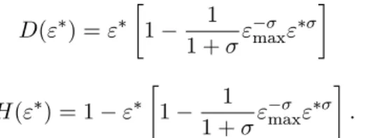
D(" ) + Z "(i) " "(i)dF(") + Z "(i)>" "tdF(") (22) H(" ) Z "(i)>" "(i)dF(") Z "(i)>" "tdF("); (23) 2 4
which satisfy 0< D(" )<1 and D(" ) +H(" ) = 1.25
A general equilibrium is de…ned as the sequences of aggregate variablesf"t; ct; kt+1; Nt; yt; wt; rtg, such that (i) given pricesfwt; rtg, households maximize utilities; (ii) given pricesfwt; rtg, …rms max-imize pro…ts; (iii) the law of large numbers hold; (iv) all markets clear: st=ktand RNt(i)di=Nt; and (v) the standard transversality condition hold:
lim
T!1E0
T(1 +g)kT+1
cT
= 0: (24)
De…ne the disposable income as }t rtst+wtNt+vt, which includes labor income, capital gains, and lump-sum pro…t income. Hence, the aggregate wealth income is related to disposable income by the relation,xt=st+}t. Using this de…nition, the consumption function and the saving function together imply the household budget identity,
ct+ (1 +g)st+1 st=}t: (25) Namely, consumption plus net savings (i.e., net wealth accumulation) equals disposable income. The aggregate saving rate can thus be de…ned as the ratio of net savings to disposable income:
t St+1 St rtSt+WtNt+Vt = (1 +g)st+1 st }t : (26)
Because of constant returns to scale, the pro…t income vt = 0. Sincest =kt, wt = (1 )Nytt, and rt+ = yktt, the household budget identity then becomes
ct+ (1 +g)kt+1 kt=yt kt; (27) where yt kt = }t is an alternative expression of disposable income. This aggregate household budget identity is also the goods market clearing condition. The de…nition of saving rate in equation (26) in general equilibrium becomes
t
(1 +g)kt+1 kt
yt kt
; (28)
which is identical to the de…nition adopted by Chen, Imrohoroglu, and Imrohoroglu (2006). The system of equations that determine the general equilibrium of the model consists of equa-tions (2), (3), (4), (16), (19), (20), (27), and the transversality condition (24). It can be easily con…rmed that this dynamic system has a unique saddle path near the steady state; that is, the
system has exactly the same number of stable roots as the number of state variables.26 Hence, these seven equations plus the transversality condition uniquely solve for the equilibrium path of
f"t; ct; kt+1; Nt; yt; wt; rtg, given the distribution of "t, the path of fgtg, and the initial condition
k0.
3
Steady-State Analysis
A "steady state" is de…ned as a situation without aggregate uncertainty wherein all variables and distributions in the transformed economy are time invariant. In a steady state the TFP growth rategt=g for allt. It can be shown that the transformed model has a unique steady state. In the steady state, equations (16), (19), (20), and (27) become
1 +g= (1 +r)R(" ) (29)
c=D(" )x (30)
(1 +g)k=H(" )x (31)
c+gk=y k; (32) respectively, where x=k+}.
In equation (29), 1 +g represents the opportunity cost of saving (the opportunity cost of not consuming the growing income today increases with the rate of income growth), and(1 +r)R(" )is the e¤ective rate of return to saving. Because saving provides liquidity to bu¤er unexpected shocks, its e¤ective rate of return is compounded by the liquidity premium R(" )>1. In equilibrium, the marginal cost of saving equals its marginal bene…ts.
Using equation (31) and realizing thatH= 1 Dgivesx= g1++Dg}. Substituting this relationship into equations (30) and (32) gives the aggregate consumption and saving as functions of disposable income:
c= (1 +g)D
g+D } (33)
gk= 1 (1 +g)D
g+D }: (34)
Therefore, the marginal propensity to consume from disposable income is given byM P C (1+g+gD)D, which is less than 1because D <1, provided that g >0. The aggregate saving rate is given by
= 1 (1 +g)D(" )
g+D(" ) : (35)
2 6By equation (16), the cuto¤"
t is stationary along a balanced growth path as long as the growth rate gt is
The saving rate depends positively on growthg. In particular, we have = 0ifg= 0, and >0if
g >0.27 Note that the saving rate depends on the cuto¤, which a¤ects the distribution of wealth across households. The cuto¤ in turn depends on the growth rate.
Proposition 2 If is small enough, an interior solution of the optimal cuto¤ " exists and is uniquely determined by the following implicit equation:
1 +g
R(" ) = 1 + g+ + (1 +g)
D(" )
H(" ) : (36)
Proof. Equation (29) implies a relationship for output-to-capital ratio: (1 +g) = 1 + yk R(" ). Equations (30) and (31) imply the consumption-to-capital ratio, kc = (1 +g)HD, which can be sub-stituted into the resource constraint (32) to obtain another equation for the output-to-capital ratio:
g+ + (1 +g)DH = yk. Combining these two restrictions yields equation (36).
Because @R@"(" ) > 0, the left-hand side (LHS) decreases monotonically with " . In particular, since" 2[0; "max]and"max>1 , the LHS has a minimum equal toLHS("max) = +1+"maxg <1 +g
and a maximum equal to LHS(0) = (1 +g). On the other hand, because DH(("" )) is monotonically increasing in" , the right-hand side (RHS) has a maximum equal to in…nity at" ="max (because
H("max) = 0) and a minimum given by h1 + g+ + (1 +g)1 i. That is, the RHS is an upward-sloping curve.
Hence, as long as the maximum of the LHS exceeds the minimum of the RHS:
1 +g > 1 + g+ + (1 +g)
1 ; (37)
a unique interior solution for" (g) exists and this value is a function of the growth rate. Condition (37) is clearly satis…ed if the multiplier is small enough.
3.1 Discussion
Proposition 2 shows that an interior solution for the cuto¤ exists only if the parameter is smaller than a critical value ~, where ~ is determined by setting the inequality (37) to an equality. It is clear that0<~<1. In contrast, if ~, then the minimum of the RHS of equation (36) exceeds the maximum of the LHS, and we have a corner solution of " = 0. In this case, only Case A in the proof of Proposition 1 is relevant, so we have st+1(i) > 0 and t(i) = 0 for all i. That is,
2 7
Although net changes in the saving stock are zero (s s= 0) in the steady state ifg= 0, the stock-to-income
the borrowing constraint never binds. Thus, equation (12) implies that t(i) is independent of i. Equations (10) and (9) then implyct(i) =wt, which is also independent ofi. In other words, when is large enough, because the extent of idiosyncratic risk is small, agents are able to perfectly smooth their consumption through saving.28 It can be shown that in this case the aggregate allocation of the model is similar to that of a representative-agent model. In the rest of the paper, we consider only the case where <~.
With the cuto¤" determined, the capital-to-output ratio can then be derived from equation (29) through the link of interest rate and marginal product of capital,
k y =
R(" )
1 +g (1 )R(" ): (38)
Recall that in a standard, representative-agent neoclassical growth model with no borrowing con-straints, the steady-state capital-to-output ratio is given by
k
y = 1 +g (1 ): (39)
Hence, at the aggregate level the current model di¤ers from the standard growth model by the liquidity premium R(" ) 1, which arises because of the possibility of binding borrowing constraints and precautionary saving motives. If the variance of the idiosyncratic shocks approaches zero (i.e., the idiosyncratic uncertainty vanishes), then the liquidity premium approaches zero and
R(" ) ! 1 in the limit. Thus, borrowing constraints do not bind and the model reduces to a standard growth model in the limit. This reveals the design of the model: The setup makes it easy to compare this model with standard growth models regarding the in‡uence of borrowing constraints on the growth-saving relationship.
Using equation (38), we can also express the saving rate alternatively as
= g k y 1 ky = gR(" ) 1 +g (1 + )R(" ): (40)
Without precautionary saving motives, as in the case of a representative-agent growth model, the saving rate becomes
o = g
1 +g (1 + ) < : (41)
Notice the following implications:
2 8
(1) Since R(" ) > 1, equations (38) and (39) suggest that the steady-state capital-to-output ratio with uninsured risk and borrowing constraints is larger than that in standard growth models. This point is noted by Aiyagari (1994).29
(2) @@go >0. That is, in a standard neoclassical growth model, the saving rate is an increasing function of TFP growth. The intuition is that higher TFP growth raises the rate of returns to capital and induces higher investment demand. Thus, the saving rate of households increases in equilibrium due to a higher real interest rate. That is, high growth leads to high saving, as in the data. This prediction is consistent with the numerical simulations of Chen, Imrohoroglu, and Imrohoroglu (2006) for the Japanese economy under the assumption of perfect foresights.30
(3) Precautionary saving not only generates a higher saving rate for any given level of growth rate (i.e., > o), it also magni…es the positive relationship between growth and saving in the neoclassical model. That is, the cross-partial derivative @g@R@ 2 is positive, because @@g >0(takingR
as given) and @R@ >0 (taking g as given); hence, if in addition dRdg >0, then borrowing constraints enhance the positive e¤ect of growth on saving. That is, if the liquidity premium is an increasing function of growth, then borrowing constraints magnify the positive relationship between growth and saving. This is ultimately the case because income growth induces consumption growth, which tightens borrowing constraints and raises the liquidity premium. This point is easier to grasp if the real interest rate is constant. In such a case, equation (29) indicates thatR(" ) rises with g.
(4) Because of higher saving rates, the equilibrium interest rate in our model will be lower than that in the standard growth model.
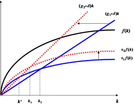
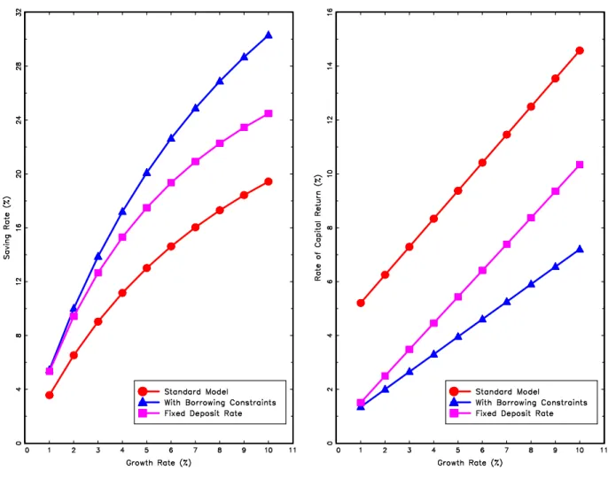
Figure 1 presents a graphic illustration of the e¤ects of growth on saving. Consider the standard growth model …rst. In the graph, a higher TFP growth fromg1 tog2 rotates the investment curve
to the left from (g1+ )k to (g2+ )k and decreases the steady-state capital stock per e¤ective
worker fromk1 tok0. As a result, consumption per e¤ective worker would fall below the modi…ed
golden-rule level if the saving rate remain unchanged at 1. Hence, a higher saving (investment)
rate is called for to raise the steady-state capital stock to k2 so that consumption per e¤ective
worker can be higher than it would be without the adjustment in the saving rate. However, in the new steady state the capital stock is still lower than before (k2 < k1), because increasing the saving
rate further would be so costly that the rate of return to saving is less than the marginal cost:
(1 +r) <1 +g. Therefore, the saving rate will increase only to the point where the discounted equilibrium real interest rate equals the growth rate.
2 9
Aiyagari (1995) argues that taxing capital is optimal in this type of incomplete-market models because of too much savings.
3 0However, in the standard neoclassical growth model the real interest rate increases with TFP growth and is about
Figure 1. E¤ects of Growth on Saving.
With borrowing constraints, the upward shift in the saving curve ( 1f(k)) is larger because a
lower capital stock raises the liquidity premium (as savings are a bu¤er stock to self-insure against idiosyncratic uncertainty), which induces the saving rate to rise further. This results in a higher steady-state capital stock thank2 (i.e., a lower real interest rate), which is dynamically ine¢ cient
because it yields lower consumption per e¤ective worker. Hence, as argued by Aiyagari (1994, 1995), taxing capital (or the rate of return to savings) would be optimal when there exist precautionary saving motives. However, our analysis here suggests that the optimal capital tax rate should be an increasing function of the growth rate.
3.2 Calibration
To facilitate quantitative evaluation of the model, we calibrate the model by assuming that "t(i) follows the power distribution, F(") = ""(i)
max , with support "(i)2[0; "max] and the shape para-meter 2 (0;1). We set the upper-bound parameter "max = 1+ (1 ) to ensure E"= 1 .
With this speci…cation, we have
R(" ) = 1 + 1
1 + "max"
1+ (42)
D(" ) = +" 1 1
H(" ) = 1 " 1 1
1 + "max" : (44)
The model’s structural parameters are calibrated as follows: The time period is a year, the time discounting factor = 0:96, the output elasticity of capital = 0:4, and the rate of capital depreciation = 0:1. As a benchmark, we pick = 0:1 and = 0:15. These values imply that the Gini coe¢ cient of …nancial wealth in the model, (1 +r)s(i), is0:79. This value roughly matches that of the major emerging economies in terms of wealth inequality. For example, the Gini coe¢ cient of wealth is 0:71 for Thailand, 0:76 for Indonesia, and 0:78 for Brazil (see, e.g., Davies et al., 2006). The reported Gini coe¢ cient for China is 0:55, which is likely signi…cantly underestimated; the true value might be somewhere close to that in Indonesia and Brazil.31 The calibrated parameter values are summarized in Table 1.
Table 1. Calibrated Parameter Values Parameter
Value 0:96 0:4 0:1 0:1 0:15
Table 2 presents the quantitative e¤ects of growth and borrowing constraints on saving rates. In Table 2, Model A represents the counterpart representative-agent neoclassical growth model (called a "standard growth model" in this paper), and Model B represents the heterogenous-agent model with borrowing constraints. Consider the standard growth model …rst (the middle row). The table shows that high growth leads unambiguously to high saving. For example, when the growth rate is at1%per year, the saving rate is less than4%; when the growth rate increases to10%per year, the saving rate rises to nearly 20%. Thus, theory predicts that high growth leads to high saving, which is consistent with the data, but in sharp contrast to PIH.
High growth leads to high saving in the standard growth model primarily because TFP growth enhances the productivity of capital, which raises the demand for investment, which in turn raises the interest rate and consequently leads to increased saving in equilibrium. In contrast, the con-ventional PIH is presented in a partial-equilibrium framework with a constant real interest rate, so high growth is not accompanied by high asset returns. Thus, consumers have no incentives to increase saving but opt to raise their marginal propensity to consume when permanent income rises.
Table 2. Saving Rate ( ) as a Function of Mean Growth (g)
g 1% 2% 3% 4% 5% 6% 7% 8% 9% 10%
Model A 3:6% 6:5% 9:0% 11:2% 13:0% 14:6% 16:0% 17:3% 18:4% 19:4%
Model B 5:4% 10% 13:9% 17:2% 20:1% 22:6% 24:9% 26:9% 28:7% 30:3%
Model A, standard growth model; Model B, with borrowing constraints.
3 1
Borrowing constraints can signi…cantly amplify the neoclassical growth e¤ect on saving. The bottom row in Table 2 shows that with borrowing constraints, the saving rate not only is much higher than in the standard model at each corresponding rate of growth, but the gap also increases with the growth rate. For example, when the growth rate is at 1% per year, the saving rate is
5:4%in Model B, which is 1:8percentage points higher than that in Model A. However, when the growth rate is at 10%per year, the saving rate is30:3%in Model B, which is about11 percentage points higher than that in Model A. This implies that borrowing constraints magnify the positive e¤ect of growth on saving.32
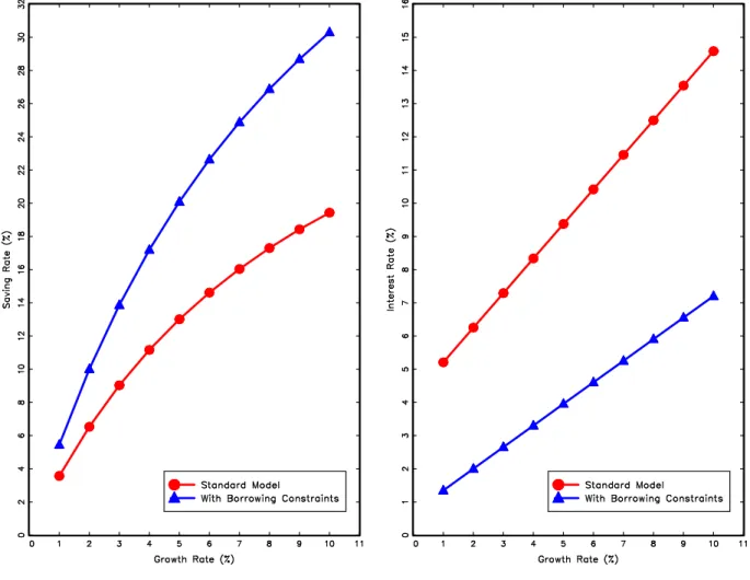
Figure 2. The Growth E¤ects on Saving and Interest.
The information in Table 2 is graphed in the left panel in Figure 2, where the line with circles represents the standard growth model (Model A), and the line with triangles the model with borrowing constraints (Model B). It shows that (i) high growth leads to high saving in both models,
3 2Borrowing constraints per se will induce a higher saving rate because of the bu¤er-stock role of savings, other
things equal. However, if there were no ampli…cation e¤ects, borrowing constraints would generate only a constantly higher saving rate than the standard growth model when the growth rate rises, instead of an increasingly higher rate, as shown in Table 2.
but (ii) the e¤ects are much stronger in Model B than in Model A and the multiplier e¤ect rises with growth.
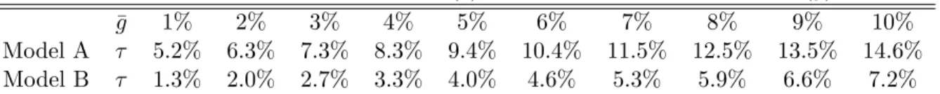
Borrowing constraints not only signi…cantly magnify the growth e¤ect on saving, but also mit-igate the growth e¤ect on interest rates. Table 3 shows that the real interest rate increases with growth in the standard model (Model A). Since a higher TFP growth implies a higher opportunity cost of saving, the rate of return to saving (the real interest rate) must also increase accordingly to induce a higher saving rate. With borrowing constraints (Model B), however, the real interest rate not only is signi…cantly lower than in the standard growth model at every level of growth, but also increases less rapidly with growth. For example, when the growth rate is1% to 3%, the implied real interest rate is about 5% to 7% without borrowing constraints (Model A), but only about 1%to3%with borrowing constraints (Model B). Also, when the growth rate rises to8%to
10%, the implied interest rate jumps up to13% to15%without borrowing constraints (Model A), but increases only to about6%to7%with borrowing constraints (Model B). The intuition is that precautionary saving results in a higher steady-state capital-to-output ratio, so the real interest rate is lower than in the standard model for any given growth rate. In addition, since the liquidity premium (R) rises with growth, the strength of precautionary saving also increases with growth, hence leading to much higher capital-to-output ratios and more subdued real interest rates.
Table 3. Equilibrium Interest Rate (r) as a Function of Mean Growth (g)
g 1% 2% 3% 4% 5% 6% 7% 8% 9% 10%
Model A 5:2% 6:3% 7:3% 8:3% 9:4% 10:4% 11:5% 12:5% 13:5% 14:6%
Model B 1:3% 2:0% 2:7% 3:3% 4:0% 4:6% 5:3% 5:9% 6:6% 7:2%
Model A, standard growth model; Model B, with borrowing constraints.
The information in Table 3 is graphed in the right panel in Figure 2, where triangles represent the model with borrowing constraints (Model B) and circles the model without borrowing constraints (Model A). Clearly, not only does the line with borrowing constraints lie signi…cantly below that without borrowing constraints at all levels of growth rates, its slope is also less steep.
4
Dynamic Analysis
This section examines the relationship between growth and saving under transitional dynamics. We consider two scenarios. In the …rst scenario, there is no aggregate uncertainty (gt = g), and we study behaviors of the saving rate and its relationship to growth when an economy starts out "poor", in the sense of having a capital stock below the steady state. We show that the model with borrowing constraints will have not only a higher growth rate but also a signi…cantly higher saving rate along the path converging to the steady state than the model without borrowing constraints,
although both models share the same steady state and rate of TFP growth. Since di¤erent degrees of borrowing constraints lead to di¤erent steady states, to ensure that the two model economies converge to the same steady state, we assume that in the borrowing-constrained economy the constraints are gradually reduced (by decreasing the variance of the idiosyncratic shocks, ) along the transitional path so that they no longer bind in the long run.33 The other parameters are calibrated to the same values as shown in Table 1, and the steady-state rate of TFP growth is set tog= 0:04 for both economies.
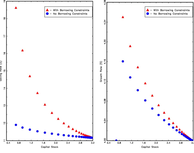
Figure 3. Transitional Dynamics.
Figure 3 depicts the saving rate (left panel) and the growth rate of investment (right panel) as a function of the capital stock for the two economies. The dots represent equally spaced points in time as the system evolves toward the shared steady state. The triangle symbols represent the model with borrowing constraints, and circles the counterpart model without borrowing constraints. Both models start with the same level of capital stock, but the model with borrowing constraints starts
3 3Namely, we have
with = 0:15 in the …rst period and this value increases over time (in every subsequent period) until it becomes large enough so that the two models converge to the same steady state in the long run.
Figure 3 shows that an initially poor economy will have both a higher-than-steady-state saving rate and a higher-than-steady-state growth rate, regardless of borrowing constraints. However, borrowing constraints reinforce this positive relationship between saving and growth so that the borrowing-constrained economy will exhibit a much higher saving rate and a moderately higher growth rate than the counterpart economy at any point in time.34 For example, the saving rate is
about 7 percentage points higher and the growth rate is about0:1 percentage points higher with borrowing constraints than without in the initial period. The intuition for this pattern is that bor-rowing constraints induce excessive saving, and the lower the capital-to-output ratio, the greater is the need for a bu¤er stock and the larger is the implied liquidity premium, which results in stronger precautionary saving, more rapid capital accumulation, and higher growth along the transitional path, even though the TFP growth rate is the same (4% a year) across the two economies.
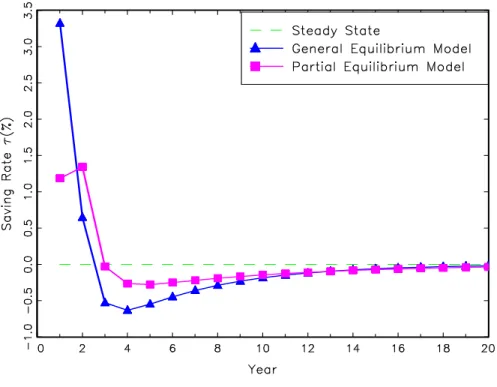
Figure 4. Impulse Responses of Saving to1% Growth Shock.
3 4Since time is discrete, we assume that in the initial period the growth rate equals the steady-state rate and there
In the second scenario, we introduce aggregate uncertainty and study the impulse responses of the saving rate to transitory TFP growth shocks. A transitory increase in the growth rate implies that income rises permanently from one level to another but not its growth rate. We use the growth process speci…ed in equation (1) to drive the model by setting the mean annual growth rate to g = 0:04 with persistence g = 0:2, consistent with postwar U.S. data. Figure 4 shows the responses (percentage deviations) of the saving rate ( t) to a 1 standard-deviation transitory increase in the growth rate,gt. Since the transformed model is solved by the method of log-linearization around the steady state, all changes in Figure 4 represent percentage deviations relative to the steady state.
The top-left panel in Figure 4 depicts the standard growth model, and the bottom-left panel the borrowing-constrained model. In either case, the saving rate rises after a positive shock to TFP growth. This happens because the higher rate of returns to capital induces investment demand and stimulates saving.35 Therefore, in sharp contrast to the prediction of the PIH, households increase rather than decrease their saving when permanent income rises, even though the higher growth rate and the consequently higher saving rate are purely transitory.36
The above results are not sensitive to the de…nition of the saving rate adopted in this paper (equation 28). For example, if the saving rate is de…ned as the ratio of gross investment to output ( t= YItt = (1+g)kt+1yt (1 )kt), it still responds positively to a growth shock, regardless of borrowing constraints (see the top-right and bottom-right panels in Figure 4). These analyses suggest that consumption growth responds less than one for one to income growth, whereas investment growth (saving) responds more than one for one to income growth. Hence, once the interest rate becomes endogenous, there does not exist the so called "excess smoothness puzzle" of consumption relative to income discussed in the consumption literature.37
A Deeper Puzzle. However, here arises another puzzle: In the general-equilibrium models pre-sented previously, the real interest rate is also the rate of return to capital; hence, high TFP growth leads to high saving through a high real interest rate. But the empirical evidence suggests that for fast-growing emerging economies the rate of return to capital may be extremely high but the interest rates facing households may be extremely low. For example, the average 3-month nominal deposit rate in China was about 3:3%per year (the average 1-year rate was about 5:6% per year) from 1990 to 2006,38 suggesting negative real deposit rates, yet the average real rate of return to
capital was more than20%per year in that period (Bai, Hsieh, and Qian, 2006). In the meantime,
3 5
The absolute change in the saving rate is larger in the borrowing-constrained model because it has a higher steady-state saving rate.
3 6
However, the income level has jumped up permanently.
3 7
For more analysis on the "excess smoothness puzzle", see Wen (2009) and the references therein.
the household saving rate in that period was about 25%, the national saving rate was about40%, and the average growth rate of real GDP per capita was about 10% per year. The situation is similar in Japan. During the high-growth and high-saving period of Japan in the 1960-70s, the average nominal 3-month deposit rate was about4%,39 and the average after-tax real rate of return to capital was above 16%, whereas the average household saving rate was about17%, the national saving rate was about20%, and the average growth rate of real income was above10%.
In addition, in both economies (Japan and China) during their respective high-growth periods, bank deposits have been the major means of saving for households, as well as the most important source of funds for …rms’investment. For example, in China, bank deposits accounted for 72% of total household …nancial assets in 2004 and 2005. In contrast, the total share of bonds and stocks accounted for less than 10% of household …nancial assets in that period. On the other hand, the share of bank loans in total corporate debt was about64%in 2004 and 2005, while the total share of corporate bonds and stocks was only around15% in that period.
Therefore, regardless of how interest rates are kept low in fast-growing economies, the puzzle is not just why high saving is positively correlated with high growth, but why high saving is possible under low interest rates. Namely, why would households save excessively to …nance …rms’ investment when the returns to their savings are so low and do not re‡ect the high returns to capital or TFP growth?40 We address this puzzle in the next section.
5
Fixed Deposit Rates
In developing economies, because of incomplete markets and various forms of …nancial repression (including distorted government banking regulations and monetary policies), large spreads may exist between deposit rates that households receive for their savings and the true rates of returns to capital that …rms receive for their investment. If such spreads exist, how do they a¤ect the relation-ship between saving and growth? This section analyzes this issue by conducting a counterfactual experiment.
5.1 With Capital
Suppose that the real interest rate faced by households is not the same as the marginal product of capital. In particular, suppose households have no access to investment opportunities except earning a low, …xed real interest rate (r) on their deposits at …nancial intermediaries. On the other hand, …rms must pay the market real interest rate (rt) to obtain loans, and banks earn
3 9
The real deposit rate is negative because the average in‡ation rate was also above6%in Japan in that period.
4 0This puzzle may be related to the well-known empirical failure in the literature to identify a signi…cantly positive
"monopolistic" pro…ts from the spread in rates of returns, (rt r)st 0.41 For simplicity, assume that the pro…ts,vt= (rt r)st, are redistributed as lump sum to households.
In a standard growth model, a …xed deposit rate is inconsistent with general equilibrium because the equilibrium condition,
1 +g= (1 +r); (45)
must hold to ensure positive household saving in the steady state. This condition will be violated when the growth rate rises — that is,1 +g > (1 +r) — so household saving will become zero (or negative if borrowing is allowed) and the marginal product of capital will become in…nity. Hence, investment demand will drive up the deposit rate in equilibrium to induce positive saving. So a …xed deposit rate below the market interest rate cannot constitute an equilibrium in a standard growth model.
However, in models with uninsured risk and borrowing constraints, a …xed deposit rate below the market interest rate can be supported by general equilibrium. Because the liquidity premium,
R(" ), can rise endogenously with growth, equation (29) can continue to hold in equilibrium even with a …xed interest rate:
1 +g= (1 +r)R(" ); (46) where the cuto¤" (g) is a function of growth. This equation shows that if the deposit rate lies below the market real interest rate, the liquidity premium will rise so that the e¤ective rate of return to saving increases to balance the marginal costs and bene…ts of saving.
This current model with the spread in the rates of returns can be solved exactly as discussed in Section 2. In equilibrium, we still have the capital market-clearing condition, st = kt; namely, the supply of capital equals its demand.42 In the steady state, we have the following analogous relationships and decision rules:
c=D(" ) [(1 )k+y] (47)
(1 +g)k=H(" ) [(1 )k+y] (48)
c+gk=y k (49)
r = y
k : (50)
The above equations imply that the saving rate is still determined by the formula in equation (35):
= 1 (1+g+gD)D. However, the implied value of the saving rate given by this equation now di¤ers
4 1
In China, all banks are state owned and the government has monopoly power on setting the deposit rates and loan rates. In Japan, although banks are privately owned, the government nonetheless had great in‡uence on banks’ interest rates in the 1950-70s.
4 2
Because of the below-equilibrium deposit rate, the demand of capital is "rationed." This implies that the marginal
product of capital exceeds the real deposit rater. The pro…ts from the spread are earned by banks by assumption,
from that given by equation (40) because the deposit rate (r) in equation (46) is no longer equal to the marginal product of capital, r = yk . Hence, the value of the cuto¤ (" ) determined by equation (46) di¤ers from that in the previous model. In particular, with a …xed deposit rate below the market rate, the optimal cuto¤" is higher and increases faster as g rises. That is, for any given level of the growth rate, the portion of the population with positive saving is smaller in the current model with a low …xed deposit rate.
Figure 5. E¤ects of Fixed Deposit Rate.
In Figure 5, the line with squares in the left-panel shows the relationship between saving and growth when the real deposit rate is …xed at 1% per year. For comparison, in Figure 5 we also include the same curves shown in Figure 2. The left-panel in Figure 5 shows that, even with such a low and …xed deposit rate, households still save signi…cantly more of their disposable income than they do in the standard growth model at various levels of the growth rate (compare the two lines with squares and circles), although the saving rates are lower than those in the counterpart model without the distorting interest spread (the line with triangles). For example, when the
growth rate is about 3% a year, the saving rate in the standard growth model without borrowing constraints is about9%; however, this rate is about13%in the current model despite an essentially zero deposit rate. Therefore, income uncertainty and borrowing constraints are able to generate excessive savings even under low interest rates.
More importantly, thanks again to borrowing constraints, as the growth rate increases, the saving rate in the current model also rises accordingly, despite the low and …xed deposit rate. That is, even though TFP growth does not transmit to the rate of returns to household savings, the saving rate still increases rapidly with economic growth. For example, when the rate of income growth increases from 3% to10% a year, the saving rate increases from 13% to25%. The reason behind this substantial rise in saving is that TFP growth a¤ects real wages, and a faster wage growth leads to a lower bu¤er stock-to-income ratio. Hence, the liquidity premium rises, which induces a higher saving rate. That is, uninsured risk and borrowing constraints make the marginal propensity to save positively dependent on permanent income due to a rising liquidity premium with income growth. Hence, even if the real deposit rate is …xed at extremely low levels, households still opt to increase their propensity to save when permanent income increases. Similar results hold even if the real deposit rate is negative.43
On the other hand, the right-panel in Figure 5 shows that the real rate of return to capital (the marginal product) in the current model with a …xed deposit rate (the line with square symbols) is higher than that in the counterpart model with borrowing constraints and a ‡exible rate (the line with triangles), and it rises faster when the growth rate increases. This explains why fast-growing economies may simultaneously exhibit low deposit rates and high (and apparently undiminished) rates of returns to capital.
The property that the marginal propensity to save depends positively on the level of permanent income is the sole consequence of uninsured risk and borrowing constraints. That is, uninsured risk and borrowing constraints can completely alter the PIH and generate exactly the opposite prediction of the PIH. The intuition is that with uninsured risk and borrowing constraints, a higher income growth (g) induces a larger liquidity premium (R) because of a lower bu¤er stock-to-‡ow ratio and thus a tighter borrowing constraint, which results in a higher e¤ective rate of return to saving.
5.2 Without Capital
This powerful e¤ect of precautionary saving on the growth-saving relationship can manifest itself even in a simpler equilibrium framework where there is no capital and both the real interest rate and the real wage are exogenous. For example, consider the special case where = 0and household
4 3
The liquidity premium has an upper bound given byR( ) +"max, which imposes a lower bound on the deposit
rate,r 1
savings are simply inventories that earn a constant real interest rate r. The production function then becomes Yt = ZtNt. The real wage then becomes completely exogenous, Wt = Zt, which grows over time at the rate gt. Since the household’s maximization program (5) has not changed, this "partial-equilibrium" model44 has closed-form solutions analogous to equations (46) through
(49):
1 +g= (1 +r)R(" ) (51)
c=D(" )x (52)
(1 +g)s=H(" )x (53)
c+gs=}; (54)
where x=s+} and } =rs+wN +v. Hence, the saving rate is still given by the same formula,
= 1 (1+g+gD)D, and the relationship between saving and growth is identical to that implied by the graph in the left panel in Figure 5 (i.e., the line with squares).45
Figure 6. Impulse Responses of Saving to1% Growth Shock.
4 4
With a little abuse of language, we call this simpler model "partial-equilibrium" model even though it is not, which helps to distinguish this model from the model with …xed deposit rate and the model with ‡exible market-determined interest rate.
4 5Note that the optimal household saving stock in this simpler model would be zero without idiosyncratic risk and
borrowing constraints. That is, if"(i) = 1 andg r, we would havest+1(i) = 0for alliandt. This is consistent