The Thirty-Third AAAI Conference on Artificial Intelligence (AAAI-19)
Learning Optimal Classification Trees
Using a Binary Linear Program Formulation
Sicco Verwer
Delft University of Technology The Netherlands [email protected]
Yingqian Zhang
Eindhoven University of Technology The Netherlands
Abstract
We provide a new formulation for the problem of learning the optimal classification tree of a given depth as a binary linear program. A limitation of previously proposed Math-ematical Optimization formulations is that they create con-straints and variables for every row in the training data. As a result, the running time of the existing Integer Linear pro-gramming (ILP) formulations increases dramatically with the size of data. In our new binary formulation, we aim to cir-cumvent this problem by making the formulation size largely independent from the training data size. We show experimen-tally that our formulation achieves better performance than existing formulations on both small and large problem in-stances within shorter running time.
Introduction
Decision trees (Breiman et al. 1984) have gained increas-ing popularity these years due to their effectiveness in solv-ing classification and regression problems and their capa-bility to explain prediction results. Learning an optimal de-cision tree with a predefined depth is NP-hard (Hyafil and Rivest 1976). Hence, greedy based heuristics such as CART (Breiman et al. 1984) and ID3 (Quinlan 1986) have been widely used to construct sub-optimal trees. Recent years have seen an increasing number of work that employ various Mathematical Optimization methods to build better qual-ity decision trees, e.g., (Bennett and Blue 1996; Bessiere, Hebrard, and O’Sullivan 2009; Verwer and Zhang 2017; Bertsimas and Dunn 2017; Silva 2017; Dash, G¨unl¨uk, and Wei 2018; Blanquero et al. 2018a; 2018b; Firat et al. 2018). An advantage of these Mathematical Optimization based approaches is that they are able to employ the powerful optimization solvers to find decision trees. This power has led to interesting new approaches for learning models and rules, see e.g., (Bessiere, Hebrard, and O’Sullivan 2009; De Raedt, Guns, and Nijssen 2010; Narodytska et al. 2018; Verwer, Zhang, and Ye 2017). In addition, the mathemati-cal optimization models allow flexibility on modeling dif-ferent learning objectives. For instance, (Verwer and Zhang 2017) incorporate constraints in the proposed Integer Lin-ear Programming (ILP) model to lLin-earn discrimination-aware classification trees. In this paper, we focus on the problem
Copyright c2019, Association for the Advancement of Artificial Intelligence (www.aaai.org). All rights reserved.
of learning optimal classification trees of given depths such that the total classification error is minimized on the training data.
A limitation of the state-of-the-art Mathematical Opti-mization formulations for this problem is that they cre-ate constraints and variables for every row in the training data (Verwer and Zhang 2017; Bertsimas and Dunn 2017). Consequently, the solving time of finding decision trees in-creases dramatically with the problem size.
We formulate the problem of constructing the optimal de-cision tree of a given depth as anbinary linear program. We call our method BinOCT, a Binary encoding for constructing Optimal Classification Trees. Our novel formulation models the selection of decision threshold via a binary search pro-cedure encoded using a type of big-M constraints. This re-quires a very small number of binary decision variables and is therefore able to find good quality solutions within limited time. Noteworthy is that the number of decision variables is largely independent of the number of training data rows: it only depends logarithmically on the number of unique feature values. Furthermore, our formulation requires fewer constraints than existing approaches. Although this number still depends linearly on the number of data rows. We show using experiments that BinOCT outperforms existing MO based approaches on a variety of data sets in terms of accu-racy and computation time.
Related work
Many studies have investigated the interplay of data min-ing and machine learnmin-ing with mathematical modelmin-ing techniques, see overview in e.g. (Bennett and Parrado-Hern´andez 2006). In this paper, we are interested in us-ing mathematical optimization methods in order to increase learning performance. For instance, (Bennett and Mangasar-ian 1993) use linear programming for determining linear combination splits within two-class decision trees. (Chang, Ratinov, and Roth 2012) propose a Constrained Conditional Model (CCM) framework to incorporate domain knowledge into a conditional model for structured learning, in the form of declarative constraints. CCMs solves prediction prob-lems. (Uney and Turkay 2006) build a mixed integer pro-gram for multi-class data classification.
encoded as disjunctive linear inequalities, and non-linear ob-jective functions are introduced to minimize errors. (Norouzi et al. 2015) link the decision tree optimization problem with the problem of structured prediction with latent vari-ables, and use stochastic gradient descent to optimize an upper bound on the empirical loss of the tree’s predic-tions. (Dash, G¨unl¨uk, and Wei 2018) propose a mathemat-ical optimization model for learning boolean decision rules in disjunctive form or conjunctive normal form. The pro-posed model takes into account the trade-off between ac-curacy and the simplicity of the chosen rules and is solved via a column generation method. (Blanquero et al. 2018a; 2018b) use a continuous optimization formulation to learn classification trees, where random decisions are made at internal nodes of the tree. Their approach is essentially a randomized optimal version of CART. (Rhuggenaath et al. 2018) build a mixed integer linear program to learn fuzzy decision trees, where split decisions on the internal nodes of a tree are not crisp. (Firat et al. 2018) apply column gener-ation techniques in constructing univariate binary classifica-tion trees. By using threshold sampling on decision nodes of the tree, the proposed approach trades its optimality for speed, i.e., it is capable of handling big data sets with tens of thousands of data rows.
The most relevant work to ours are (Bertsimas and Sh-ioda 2007; Bertsimas and Dunn 2017; Verwer and Zhang 2017). In these papers, the authors formulate the problem of learning classification trees of depth K using Integer Lin-ear programs (ILP). The model proposed in (Bertsimas and Shioda 2007) is quadratic in the data set size and therefore requires a lot of preprocessing in order to reduce the number of generated constraints. The number of decision variables in the ILP model of (Bertsimas and Dunn 2017) isO(R·2K), whereRis the number of data rows. In (Verwer and Zhang 2017), a more efficient encoding is proposed for construct-ing both classification and regression trees, where the num-ber of decision variables is reduced toO(R·K). (Bertsi-mas and Dunn 2017) show their model is in general better than CART in terms of testing accuracy when the running time was set to two hours for solving each instance. (Ver-wer and Zhang 2017) also compare their model with CART. Their model outperforms CART with trees up to depth 5 on datasets of size up to 1000.
Learning optimal classification trees as binary
linear programs (BinOCT)
We assume readers to be familiar with classification trees, see, e.g., (Flach 2012). The optimization problem that we aim to solve is to find an optimal classification tree of depth K for a given dataset ofRrows andF features, such that the total classification error is minimized. The Boolean de-cisions on each internal nodes of the tree and predictions on the leaves are variables and need to be set such that the classification accuracy is optimized. We solve this problem by formulating it as a Binary Linear Program (BLP), which contains only binary decision variables.
Formulation Intuition
Our formulation for classification trees aims to reduce the dependence of the problem size with the size of the train-ing data. In existtrain-ing formulations this dependence is present in both the number of constraints and the number of sion variables, see Table 2. The number of (boolean) deci-sion variables that our formulation requires is significantly smaller than that in the previously proposed methods. More-over, this number is independent of the number of training data rows. Instead, it depends on the maximum amount of unique feature values among all features. Similarly, we also aim to minimize the number of constraints required by our formulation. Below, we first explain the key ideas required to understand our formulation using small examples. We may slightly abuse notations during explanation. At the end of this section, we provide the complete formulation.
Boolean Decision Thresholds. In contrast to earlier for-mulations that use continuous or integer decision thresholds for each internal node, we represent decision thresholds us-ing only binary variables. When the feature used in the deci-sion is binary, the formulation is intuitive, as explained be-low. Assume we are learning a tree consisting of a single decision node. Letlr,1 andlr,2 be binaries indicating that data rowrreaches leaf1in the left and leaf 2in the right branch from the root node. A row has to reach a single leaf:
lr,1+lr,2= 1.
Lettnbe a binary variable for the binary decision threshold for noden, that is, depending on the value oftn, a data row goes to the left or right branch of noden. Hence, leaf1is reached by rowrwhentn is0. Leaf2is reached by rowr whentn is1. This can be encoded by adding the following two constraints
lr,1+tn≤1andlr,2−tn≤0.
These constraints forcelr,1to be0whentnequals1andlr,2 to0whentn equals0. The first constraint then guarantees that the leaf not forced to0is reached by rowr. Note that al-though the leaf variableslare boolean, they can be modeled as continuous because the above constraints force them to be either0or1. This makes the problem significantly easier be-cause when an optimization solver is used to solve the given BLP model, continuous variables do not have to be consid-ered as branching nodes during its branch-and-bound search, i.e., they can be solved using standard linear programming.
Combining Constraints. A naive formulation based on this intuition would require a large number of constraints, i.e., at least one for every row in the training data. We sig-nificantly reduce this number by the observation that we can simply sum the above constraints of threshold checking for all data rowsrwith feature valueVf
r equal to1, i.e.,
X
r:Vrf=1
lr,1+M ·tn ≤M and X
r:Vrf=1
lr,2−M·tn≤0,
whereM =P
r:Vrf=11. Like before,lr,1= 0whentn=
rows in the training data. Although it is known that integer programming solvers can experience difficulties with such big-M formulations, in our experience and as shown in the experiments it solves much faster than creating additional constraints for every row in the training data. In the case of larger trees, we can safely add all leaves under the left and right branch to the constraints since their sum is at most1:
X
r:Vrf=1
X
i∈ll(n)
lr,i+M ·tn ≤M
X
r:Vrf=1
X
i∈rl(n)
lr,i−M ·tn ≤0, (1)
wherell(n)andrl(n)are the set of leaves under the left and right branches of noden, respectively,M =P
r:Vrf=11
andtn is a binary threshold variable for noden. An impor-tant observation is that since we force the leaf variableslr,i to be 0, these constraints can be created for every node in the tree without influencing each other. Together they represent rowr’s path to the leafiwithlr,iequal to1, i.e., not forced to0by any of the node constraints.
Integer Decision Thresholds. The node constraints above are sufficient for modeling all paths of all training data rows when the decision thresholds are boolean. A naive method to transform integer or continuous valued features to binary ones is using a unary representation that uses one variable per decision threshold. Instead, we use a binary representa-tion for the decision thresholds that requires exponentially fewer variables.
Example 1 For ease of explanation, we assume that we aim to find a single decision node nfor the following training set, which contains only one feature with 9 distinct feature values. The rows are ordered using the feature values:
feature value 0 1 2 3 4 5 6 7 8
target class + + + - - + - + +
Because there is no reason to split groups of examples that have the same label, there are4sensible thresholds we can use to split data. In theory it could occur in multivariate datasets such a split is needed to find the optimal tree. We still remove them from consideration to reduce the size of the learning problem, in this case from 8 to 4 possible thresh-olds. We model these4possible thresholds usinglog24 = 2 binary variablestn,1andtn,2as shown in Figure 1.
Thus, iftn,1is1, the threshold is one of the first two possi-ble thresholdsth(1)orth(2). In our example, such a setting implies that any rows with a feature value greater than4.5
(the2nd threshold value) cannot reach any of the leaves un-der the left branch of noden. Similarly, whentn,1is0, any rows with a feature value less then 5.5 (the 3rd threshold value) cannot reach any of the leaves under the right branch of noden. This results in the following constraints, updated from Equation (1):
X
r:th(2)<Vrf<th(4)
X
i∈ll(n)
lr,i+M·tn,1≤M
0-2 + 3-4 - 5 + 6 - 7-8 + 1
1 1 0
0
0
th(1) th(2) th(3) th(4)
Right Leaf Left Leaf
Node n
Figure 1: A decision tree with one internal node. Inside of this node, a binary search tree is used to represent one of the 4 possible threshold valuesth(1)-th(4)for Example 1. The edges on the arcs denote the value settings of the binary variablestn,i, withithe depth of the search tree. Thus set-tingtn,1to1andtn,2to0corresponds to selecting threshold th(2). The boxes show the feature value ranges and class values to the left and right of every decision threshold. A threshold setting ofth(2)forces all rows with values from the first two boxes to reach the left leaf, and all rows with values from the last three boxes to reach the right leaf.
X
r:th(1)<Vrf<th(3)
X
i∈rl(n)
lr,i−M0·tn,1≤0,
where th(i) returns the ith threshold value, and the constants M and M0 are P
r:th(2)<Vrf<th(4)1 and
P
r:th(1)<Vrf<th(3)1, respectively. Notice that these
con-straints force all rows with a feature value of5(both greater than the2nd and smaller than the3rd threshold) to either the left or right branch, depending on the setting oftn,1. Further-more, notice we do not create these constraints for rows with feature values below the lowest (th(1)) or above the high-est (th(4)) threshold. Rows with values below the minimum threshold can never follow the right branch, no matter which threshold is chosen. The reverse holds for rows with values above the largest threshold and we use separate constraints to model these extreme values, which we discuss later.
The second binary variable tn,2 is then used to force the direction for the remaining rows with values between th(1)andth(2), and betweenth(3)andth(4). Whethertn,2 forces this for the first or last range depends on the value of tn,1. We first show the first range and include the higher or-der bit oftn,1using big-M values:
X
r:th(1)<Vrf<th(2)
X
i∈ll(n)
lr,i+M·tn,1+M ·tn,2≤2·M
X
r:th(1)<Vrf<th(2)
X
i∈rl(n)
lr,i−M ·tn,2≤0,
whereM = P
r:th(1)<Vrf<th(2)1. Notice that we have to
rows with feature values in range[th(1), th(2)]cannot reach any leaf under the right branch of noden. These rows have feature values that are smaller than either threshold value. In the same way, we make the constraints for the upper range:
X
r:th(3)<Vrf<th(4)
X
i∈ll(n)
lr,i+M·tn,2≤M
X
r:th(3)<Vrf<th(4)
X
i∈rl(n)
lr,i−M ·tn,1−M ·tn,2≤0,
withM =P
r:th(3)<Vrf<th(4)1.
Example 2 Let us see the effect of the above6 constraints on our example data. For simplicity, we use the feature value also as row number, i.e., lr,i where 0 ≤ r ≤ 8, and we
assume there is only one single left leaf 1 and one single right leaf2for noden. After writing out the above defined constraints, we obtain in order:
l5,1+l6,1+ 2·tn,1≤2
l3,2+l4,2+l5,2−3·tn,1≤0
l3,1+l4,1+ 2·tn,1+ 2·tn,2≤4
l3,2+l4,2−2·tn,2≤0
l6,1+ 1·tn,2≤1
l6,2−1·tn,1−1·tn,2≤0.
The effect of settingtn,1,tn,2to1,1is thatl5,1andl6,1are
forced to0by the first constraint.l3,1andl4,1are forced to0
by the third constraint.l6,1is (again) forced to0by the fifth
constraint. Since the feature values of the last two rows are largest, the last two rows cannot end up in the left leaf, that is,l7,1 and l8,1 are always0. Similarly,l0,1,l1,1, and l2,1
are always1. This results in the following table, which we extend with all possible settings oftn,1 andtn,2. Note that
since we have two leaves, forcingli,2to be0causesli,1to
be set to1:
tn,1 tn,2 l0:2,1 l3,1 l4,1 l5,1 l6,1 l7:8,1
1 1 1 0 0 0 0 0
1 0 1 1 1 0 0 0
0 1 1 1 1 1 0 0
0 0 1 1 1 1 1 0
This correctly models which rows reach which leaves under the4different threshold settings.
In our formulation, we extend this idea to arbitrary ranges of threshold values by using a simple recursive routine to generate the corresponding constraints. We make sure that every tn,i bit of the binary encoding divides the possible threshold values in half. The firsttn,1is thus always impor-tant because it eliminates half of the possible paths of rows (that reach noden) to leaf nodes. Intuitively, this makes it easier for the solver to find solutions since it can eliminate many possible solutions by fixing only a few binary values. Notice also that the used big-M values change depending on the number of influenced rows. In this way, We obtain few constraints with very large M values but few decision vari-ables, and many constraints with small M values but several decision variables.
In the following, we use bin(f) to denote the result of our recursive routine for feature f. For each featuref, we compute the number of possible threshold valuesTf as fol-lows. We sort all unique feature values and create thresholds between every two subsequent values, unless all rows with those values belong to the same class (see the small exam-ple in Examexam-ple 1). Pseudocode for the recursive routine for each feature is given in Algorithm 1. Initially, the algorithm is called with(1, Tf,1). The algorithm returns a set (or iter-ator)b∈bin(f)over the lowerlr(b)and upperur(b)value ranges, and the requiredtn,tvariables (tl(b)) for the left and right leaf nodes.
Algorithm 1Obtaining the binary encoding value ranges
1: procedureBIN(min,max,depth) 2: Letbbe a binary value range 3: ifmax−min <= 1then
4: lr(b)= [th(min),th(max)] lower range ofb
5: ur(b)= [th(min),th(max)] upper range ofb
6: return[b] 7: end if
8: result = [b]
9: mid=FLOOR((max−min)/2.0)
10: lr(b)= [th(min),th(min+mid+ 1)] lower range 11: ur(b)= [th(min+mid),th(max)] upper range 12: tl(b)=tr(b)= [depth] include current depthtn,t
13: forb0inBIN(min,min+mid,depth+ 1)do
14: tl(b0)=tl(b0)+ [depth] includetn,tforll(n)
15: result = result + [b0] 16: end for
17: forb0inBIN(min+mid+ 1,max,depth+ 1)do
18: tr(b0)=tr(b0)+ [depth] includetn,tforrl(n)
19: result = result + [b0] 20: end for
21: returnresult 22: end procedure
Features So far, the formulation of node constraints as-sumed there is only one single feature we can choose from when determining thresholds at internal nodes. For a general case with multiple features, in order to select which feature to use in a node constraint, we add another big-M multi-plier, for all features f (1 ≤ f ≤ F) and binary ranges b∈bin(f):
M·fn,f+ X
r∈lr(b) X
l∈ll(n) lr,l+
X
t∈tl(b)
M·tn,t ≤M+ X
t∈tl(b) M
M0·fn,f+ X
r∈ur(b) X
l∈rl(n) lr,l−
X
t∈tl(b)
M0·tn,t ≤M0,
where M = P
r∈lr(b)1, M0 = P
r∈ur(b)1, and ll(n) (rl(n)) is the set of noden’s leaves under the left (right) branch. The additional big-M ensures that these constraints only have effect whenfn,f is equal to1. Of course, we re-quire that exactly one feature is selected for every decision noden:
X
1≤f≤F
All that remains for modeling the nodes of the decision tree is to add constraints for rows with feature values greater than the largest threshold, or lower than the smallest threshold. These are forced to0 using only the node feature variable fn,f, for all featuresf:
M·fn,f+
X
r:maxt(f)<Vrf X
l∈ll(n)
lr,l+
X
r:Vrf<mint(f) X
l∈rl(n)
lr,l≤M,
where M = P
r:maxt(f)<Vrf1 +
P
r:Vrf<mint(f)1, and maxt(f) andmint(f) are the minimum and maximum de-cision thresholds for featuref.
Objective Function The node constraints described above model the influence of the decision variablestn,tandfn,fon which leaf nodelr,leach of the training data row reaches. We create our objective function using these leaf node (not de-cision) variables. Similarly to the node constraints, we com-bine the objective values of as many rows as possible using a big-M value. In this case, we combine all that end in the same leaf with the same target class. For all leavesland tar-get classesc:
X
r:Cr=c
lr,l−M ·pl,c≤el,c,
whereM = P
r:Cr=c1,Cris the class of row r,pl,cis a
binary decision variable indicating whether leaf l predicts classc, andel,cis the number of misclassifications for class cin leafl. Lastly, every leaf predicts exactly one class value:
X
1≤l≤L
pl,c= 1.
The BinOCT model
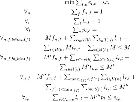
We now present the full formulation for learning optimal classification trees as follows. The objective is to minimize the total classification error. Table 1 lists the used notation.
minP
l,cel,c s.t.
∀n Pffn,f = 1
∀r Pllr,l= 1
∀l Pcpl,c= 1
∀n,f,b∈bin(f) M fn,f+Pr∈lr(b) P
l∈ll(n)lr,l+ P
t∈tl(b)M tn,t− P
t∈tl(b)M ≤M
∀n,f,b∈bin(f) M0fn,f+Pr∈rr(b) P
l∈rl(n)lr,l− P
t∈tl(b)M0tn,t≤M0 ∀n,f M00fn,f+Pmaxt(f)<f(r)
P
l∈ll(n)lr,l+ P
f(r)<mint(f)
P
l∈rl(n)lr,l≤M00 ∀l,c Pr:Cr=clr,l−M000pl≤el,c
with1 ≤ n ≤ N,1 ≤ f ≤ F,1 ≤ r ≤ R,1 ≤ l ≤
L,1 ≤ c ≤ C unless stated otherwise. How to derive the
Symbol Type Definition
n index internal (non-leaf) node,1≤n≤N l index leaf of the tree,1≤l≤L r index row in the training data,1≤r≤R f index feature in the training data,1≤f≤F c index class in the training data,1≤c≤C bin(f) set featuref’s binary encoding ranges
lr(b) set rows with values inb’s lower range,b∈bin(f) ur(b) set rows with values inb’s upper range
tl(b) set tn,tvariables forb’s ranges
ll(n) set noden’s leaves under the left branch
rl(n) set noden’s leaves under the right branch
K constant tree’s depth
N constant N= 2K−1, number of internal nodes
L constant L= 2K, number of leaf nodes
F constant number of features
C constant number of classes
R constant number of training data rows
T constant total number of threshold values
Tf constant number of threshold values for featuref
Tmax constant maximum ofTfover all featuresf
Vf
r constant featuref’s value in training data rowr
Cr constant class value in training data rowr
mint(f) constant featuref’s minimum threshold value
maxt(f) constant featuref’s maximum threshold value
M constant minimized big-M value
fn,f binary noden’s selected featuref
tn,t binary noden’s selected thresholdt
pl,c binary leafl’s selected prediction classc
el,c continuous error for rows with classcin leafl
lr,l continuous rowrreaches leafl
Table 1: Summary of notation used in the encoding.
smallest M values for different constraints and the details of equations have been described in the previous subsec-tions. All decision variables fn,f,tn,t, and pl,c are binary. The number of fn,f variables is bounded by N ·F. The number oftn,tvariables in bounded byN·log(Tmax). Note Tmaxis no more than the number of distinct values for each feature. The number ofpl,cvariables is bounded byL·C. For a depthK tree, the formulation thus requires at most N·(F+log(T))+L·C≤2k(F+C+log(T))decision vari-ables. This depends linearly on the number of features and class values, and only logarithmic on the number of possible decision boundaries. Most importantly, this is independent from the number of data rows as long as new rows do not add new features, possible thresholds, or class values.
fea-ture. For example, if a feature only has two possible values (coming from a one-hot encoding for instance), then there is only a single decision threshold and we require only a sin-gle constraint to model the node’s behavior for that feature (only the minimum and maximum value ranges). Sometimes Rwill be the dominating term, i.e., when the training data set is large and the number of possible thresholds is small.
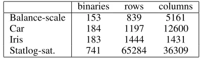
As table 3 shows, our formulation results in very few bi-nary decision variables. Even for problems with thousands of rows, we only require a few hundred binaries.
Method # decision variables # constraints
BinOCT O(2K(F+C+log(T
max))) O(R+ 2K(F·Tall+C))
DTIP O(R·K) O(R·2K−1)
OCT O(R·2K) O(2K−1(R·K+C))
Table 2: The number of decision variables and constraints used in three methods: our method BinOCT, DTIP in (Ver-wer and Zhang 2017), and OCT in (Bertsimas and Dunn 2017).Ris the number of data rows,F number of features, Cnumber of classes,Kdepth of tree.Tmaxis the maximum number of thresholds for any feature andTallis the number of all decision thresholds over all features.
binaries rows columns
Balance-scale 153 839 5161
Car 184 1197 12600
Iris 183 1444 1431
Statlog-sat. 741 65284 36309
Table 3: Sizes of depth 4 training problems (containing 50% of the data) reported by CPLEX.
Dataset R F C Tmax Tall
Balance-scale 625 4 3 4 16
Bank marketing 10% 4521 17 2 799 1690
Banknote-authentification 1372 4 2 624 1855
Car-evaluation 1728 5 4 3 14
Ionosphere 351 34 2 94 2312
Iris 150 4 2 23 56
Monks-problems-1 124 6 2 3 11
Monks-problems-2 169 6 2 3 11
Monks-problems-3 122 6 2 3 11
Pima-Indians-diabetes 768 8 2 309 857
Qsar-biodegradation 1055 41 2 437 4178
Seismic-bumps 2584 18 2 311 1120
Spambase 4601 57 2 1174 8006
Statlog-satellite 4435 36 6 80 2217
Tic-tac-toe-endgame 958 18 2 1 18
Wine 178 13 3 70 710
Table 4: The datasets used in the experiments.
Experiments
To solve classification problems, given a training dataset, We formulate the learning problem using the proposed for-mulation. The resulting BinOCT model is passed to the
optimization solver CPLEX 12.8.0, running on an AMD Ryzen machine with 16GB RAM, which returns the best solution (i.e., a classification tree with highest accuracy) it can find within the given time limit. We provide CPLEX with a priority order such that variables closer to the root of the tree get solved first. We test our method on bench-mark datasets from the UCI machine learning repository (Lichman 2013). We compare the performance of BinOCT with OCT (Bertsimas and Dunn 2017) and DTIPs (Verwer and Zhang 2017), two recently proposed ILP-based classi-fication algorithms. We use the accuracy in the cited pa-pers for comparison. We also run CART from sciki-learn with its default parameter setting (i.e., criterion=gini, split-ter=best, min samples split=2, min samples leaf=1, max leaf nodes=None), except that the maximum depths of the trees generated by CART are set to the same depths as BinOCT. In addition, as in (Bertsimas and Dunn 2017; Verwer and Zhang 2017), BinOCT is solved by CPLEX with warm starts learned from CART to investigate whether this helps find better solutions. We name it BinOCT*.
In order to compare to OCT, we use the same experi-ment settings as in (Bertsimas and Dunn 2017). For a given dataset, 50% of the dataset are used for training and 25% for testing. As we do not have hyperparameters to tune in our model, the remaining 25% are not used. The split is down randomly five times. We report the average performance of five experiments for each dataset. We chose datasets (see Ta-ble 4) containing no missing values since it is not clear how the authors of (Bertsimas and Dunn 2017) pre-processed the datasets with missing values.
The time limit for BinOCT is set to 10 minutes for each instance. In comparison, OCT used 30 minutes to 2 hours to solve each instance in (Bertsimas and Dunn 2017), and DTIPs was run at most 30 minutes in (Verwer and Zhang 2017). We learn trees with depths ranging from 2 to 4.
Our implemented models, the code, and the used training and testing data sets are available online at https://github.com/SiccoVerwer/binoct.
Results
We tested our method on 16 datasets. The number of data rows in these datasets range from 124 to 4601, and the num-ber of features from 4 to 57.
In Table 5, we report the accuracy on the training data. As explained earlier, each dataset was split randomly 5 times. The accuracy value of BinOCT and CART in the table is the average accuracy on five training sets. Since DTIPs in (Ver-wer and Zhang 2017) used the complete dataset for training, we also include in the table the reported CART results from (Verwer and Zhang 2017). The training results of OCT are absent in (Bertsimas and Dunn 2017).
Dataset BinOCT BinOCT* CART/R DTIPs BinOCT BinOCT* CART/R DTIPs BinOCT BinOCT* CART/R DTIPs
k=2 k=3 k=4
Balance-scale 73.3* 73.3* 71.7 79.2 78.7 76.5 84.8 84.1 82.9
Bank market. 10% 90.3 90.3 89.9/90.1 90.1 90.4 90.9 90.7/90.4 90.6 90.6 91.8 91.6/91.2 91.3 Banknote-auth. 93.4* 93.4* 91.7 97.8 97.7 94.6 99.4 99.7 97.4
Car-evaluation 76.9* 76.9* 76.9* 80.5 80.4 79.0 85.3 85.7 84.2
Ionosphere 91.1 91.2 91.0 94.3 94.9 93.8 96.8 97.1 96.0
Iris 96.8* 96.8* 96.8*/96* 96* 100* 100* 98.1/97.3 99.3* 100* 100* 100*/99.3 100* Monks-probl-1 83.5* 83.5* 76.8 92.6* 92.6* 81.6 99.4 99.4 86.1
Monks-probl-2 69.8* 69.8* 65.2 79.5 79.5 70.0 86.7 86.9 79.8 Monks-probl-3 93.8* 93.8* 93.8* 95.7* 95.7* 94.8 97.7 98.0 95.7
PI-diabetes 79.3 79.3 77.3/77.2 77.7 81.6 81.3 78.9/77.6 79.4 83.0 84.7 82.9/79.3 82.6
Qsar-biodeg. 80.9 81.2 80.5 83.9 85.8 85.3 84.6 89.1 88.7
Seismic-bumps 93.5 93.4 93.1 93.7 93.7 93.4 93.7 94.2 93.9
Spambase 85.6 86.7 86.0 86.1 90.2 89.6 84.8 91.9 91.6
Statlog-sat. 68.8 66.7 63.2 72.7 80.5 78.7 66.5 81.6 81.6
Tic-tac-toe 72.1* 72.1* 71.2* 79.2 77.6 75.4 85.2 85.3 84.4
Wine 97.3* 97.3* 95.7 100* 100* 99.3 100* 100* 100*
Table 5: Training accuracy of BinOCT, BinOCT* (BinOCT with CART as starting solutions), CART, R (CART in (Verwer and Zhang 2017), DTIPs. The symbol * next to the values means that the solutions are optimal. The best performing method at same depths is marked in bold.
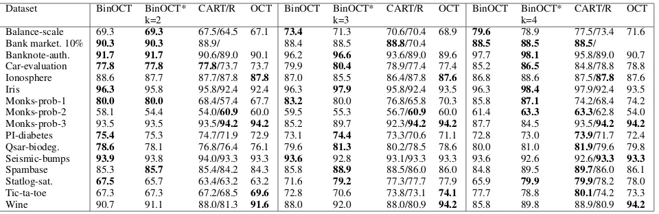
Dataset BinOCT BinOCT* CART/R OCT BinOCT BinOCT* CART/R OCT BinOCT BinOCT* CART/R OCT
k=2 k=3 k=4
Balance-scale 69.3 69.3 67.5/64.5 67.1 73.4 71.3 70.6/70.4 68.9 79.6 78.9 77.5/73.4 71.6
Bank market. 10% 90.3 90.3 88.9/ 88.4 88.5 88.8/70.4 88.5 88.5 88.5/
Banknote-auth. 91.7 91.7 90.6/89.0 90.1 96.2 96.6 93.6/89.0 89.6 97.7 98.1 95.8/89.0 90.7
Car-evaluation 77.8 77.8 77.8/73.7 73.7 79.9 80.4 78.9/77.4 77.4 85.2 86.5 84.8/78.8 78.8
Ionosphere 88.6 87.7 87.7/87.8 87.8 87.0 85.5 86.4/87.8 87.6 86.8 88.6 87.5/87.8 87.6
Iris 96.3 95.8 95.8/92.4 92.4 96.3 97.9 95.8/92.4 93.5 96.3 98.4 97.9/92.4 93.5
Monks-prob-1 80.0 80.0 68.4/57.4 67.7 83.2 80.0 76.8/65.8 70.3 85.8 87.1 74.2/68.4 74.2
Monks-prob-2 58.1 54.4 54.0/60.9 60.0 59.5 55.3 56.7/60.9 60.0 61.4 63.3 63.3/62.8 54.0
Monks-prob-3 93.5 93.5 93.5/94.2 94.2 85.2 89.7 92.3/94.2 94.2 87.7 84.5 93.5/94.2 94.2
PI-diabetes 75.4 75.3 74.7/71.9 72.9 73.1 74.4 73.3/70.6 71.1 72.8 73.0 73.9/71.7 72.4
Qsar-biodeg. 78.6 78.1 76.8/76.4 76.1 79.6 81.3 80.2/78.5 78.6 80.0 81.0 81.9/79.6 79.8
Seismic-bumps 93.9 93.8 94.0/93.3 93.3 93.6 92.8 93.1/93.3 93.3 93.6 92.6 92.6/93.3 93.3
Spambase 85.3 85.7 85.4/84.2 84.3 85.8 88.9 88.5/86.0 86.0 84.8 89.5 89.7/86.0 86.1
Statlog-sat. 67.5 65.7 63.4/63.2 63.2 71.6 79.2 77.3/77.7 77.9 65.9 79.9 79.9/78.2 78.0
Tic-ta-toe 67.3 67.3 67.2/68.5 69.6 72.8 70.6 73.8/73.1 74.1 77.7 78.8 80.1/74.2 73.3
Wine 90.7 91.1 88.0/81.3 91.6 88.0 92.0 88.0/80.9 94.2 85.8 89.8 88.9/80.9 94.2
Table 6: Testing accuracy of BinOCT, BinOCT*, CART, R (CART in (Bertsimas and Dunn 2017)) and OCT.
10 minutes. These problems have many features, classes, and possible threshold values. The performance of BinOCT and BinOCT* are comparable when learning tees of depths 2 and 3. When the model becomes large (depth 4), it is more beneficial to have a starting solution. DTIPs was also able to return optimal solutions on Iris for trees of different depths. The performance of our methods on the other two datasets is consistently higher than DTIPs, although we ran the in-stances much shorter than theirs (10 instead of 30 minutes).
In Table 6 we report the testing accuracy. For depth2and
3, BinOCT outperforms the other methods on many problem instances. Interestingly, it does not outperform OCT when it finds 100% accurate models on the training data for the Wine instances. On depth4problems, the solutions found by BinOCT are frequently outperformed by CART although it’s training accuracy is always better. This shows the strength of CART and OCT in making a trade-off between accuracy and model complexity. By purely maximizing accuracy on the training data, BinOCT is essentially overtraining.
Al-though necessary, this trade-off makes it hard to compare the quality of the different formulations. A different trade-off decision creates a different objective function and thus a different problem to solve. The different cross-validation folds and dissimilar CART performance Overall make this comparison even harder. The best we can do is compare the improvement over CART. For depth 2 and3, BinOCT or BinOCT* clearly outperforms CART, but so does OCT. For the depth 4 instances, OCT’s performance was very close or worse than their CART results. BinOCT* gives slightly better results than CART overall, but sometimes worse due to overfitting. Overall, the results are impressive as we ran only 10 minutes to achieve performance often better than OCT, which was run for 2 hours.
Conclusion
smaller than those in the state-of-the-art formulations. Im-portantly, the size of the decision variables used in our model BinOCT is independent from the size of datasets. The advan-tage of this independence has been demonstrated through a set of experiments. BinOCT, with or without starting solu-tions, gave overall better solutions than the existing formula-tions OCT and DTIPs, despite the fact that the running time of BinOCT was much shorter than OCT and DPIPs. In the future, we plan to extend our model with different learning objectives, such as adding fairness criteria. In addition, we will add a trade-off between accuracy and model complexity to the objective function. Lastly, we will investigate further improving the formulation by reducing the number of con-straints, or using approximation strategies such as selecting a subset of data rows or possible threshold values.
Acknowledgements
The work is partially supported by the NWO project Real-time data-driven maintenance logistics (project number: 628.009.012).
References
Bennett, K. P., and Blue, J. A. 1996. Optimal decision trees. Technical report, R.P.I. Math Report No. 214, Rensselaer Polytechnic Institute.
Bennett, K. P., and Mangasarian, O. L. 1993. Bilinear sep-aration of two sets inn-space. Computational Optimization and Applications2(3):207–227.
Bennett, K. P., and Parrado-Hern´andez, E. 2006. The inter-play of optimization and machine learning research.Journal of Machine Learning Research7:1265–1281.
Bertsimas, D., and Dunn, J. 2017. Optimal classification trees.Machine Learning106(7):1039–1082.
Bertsimas, D., and Shioda, R. 2007. Classification and regression via integer optimization. Operations Research
55(2):252–271.
Bessiere, C.; Hebrard, E.; and O’Sullivan, B. 2009. Min-imising decision tree size as combinatorial optimisation. In International Conference on Principles and Practice of Constraint Programming, 173–187. Springer.
Blanquero, R.; Carrizosa, E.; Molero-Rıo, C.; and Morales, D. R. 2018a. Optimal randomized classification trees.
Blanquero, R.; Carrizosa, E.; Molero-Rıo, C.; and Morales, D. R. 2018b. Sparsity in optimal randomized classification trees.
Breiman, L.; Friedman, J.; Olshen, R.; and Stone, C. 1984.
Classification and regression trees. Wadsworth International Group.
Chang, M.; Ratinov, L.; and Roth, D. 2012. Structured learn-ing with constrained conditional models.Machine Learning
88(3):399–431.
Dash, S.; G¨unl¨uk, O.; and Wei, D. 2018. Boolean decision rules via column generation. arXiv preprint arXiv:1805.09901.
De Raedt, L.; Guns, T.; and Nijssen, S. 2010. Constraint programming for data mining and machine learning. In Pro-ceedings of the Twenty-Fourth AAAI Conference on Artifi-cial Intelligence (AAAI-10), 1671–1675.
Firat, M.; Crognier, G.; Gabor, A. F.; Hurkens, C.; and Zhang, Y. 2018. Constructing classification trees using col-umn generation. arXiv preprint arXiv:1810.06684.
Flach, P. 2012. Machine learning: the art and science of algorithms that make sense of data. Cambridge University Press.
Hyafil, L., and Rivest, R. L. 1976. Constructing optimal bi-nary decision trees is np-complete. Information Processing Letters5(1):15 – 17.
Lichman, M. 2013. UCI machine learning repository. Narodytska, N.; Ignatiev, A.; Pereira, F.; Marques-Silva, J.; and RAS, I. S. 2018. Learning optimal decision trees with sat. InIJCAI, 1362–1368.
Norouzi, M.; Collins, M. D.; Johnson, M.; Fleet, D. J.; and Kohli, P. 2015. Efficient non-greedy optimization of deci-sion trees. InProceedings of the 28th International Confer-ence on Neural Information Processing Systems, NIPS’15, 1729–1737. Cambridge, MA, USA: MIT Press.
Quinlan, J. R. 1986. Induction of decision trees. Machine learning1(1):81–106.
Rhuggenaath, J.; Zhang, Y.; Akcay, A.; Kaymak, U.; and Verwer, S. 2018. Learning fuzzy decision trees using integer programming. In2018 IEEE International Conference on Fuzzy Systems.
Silva, A. P. D. 2017. Optimization approaches to supervised classification. European Journal of Operational Research
261(2):772–788.
Uney, F., and Turkay, M. 2006. A mixed-integer program-ming approach to multi-class data classification problem.
European Journal of Operational Research 173(3):910– 920.
Verwer, S., and Zhang, Y. 2017. Learning decision trees with flexible constraints and objectives using integer opti-mization. InInternational Conference on AI and OR Tech-niques in Constraint Programming for Combinatorial Opti-mization Problems, 94–103. Springer.