Pickup ion-mediated plasma physics of the outer heliosphere and very local interstellar medium

REVIEW

Pickup ion-mediated plasma physics

of the outer heliosphere and very local

interstellar medium

G. P. Zank

Abstract

Observations of plasma and turbulence in the outer heliosphere (the distant supersonic solar wind and the subsonic solar wind beyond the heliospheric termination shock) made by the Voyager Interstellar Mission and the energetic neutral atom observations made by the IBEX spacecraft have revealed that the underlying plasma in the outer helio-sphere and very local interstellar medium (VLISM) comprises distinct thermal proton and electron and suprathermal pickup ion (PUI) populations. Estimates of the appropriate collisional frequencies show that the multi-component plasma is not collisionally equilibrated in either the outer heliosphere or VLISM. Furthermore, suprathermal PUIs in these regions form a thermodynamically dominant component. We review briefly a subset of the observations that led to the realization that the solar wind–VLISM interaction region is described by a non-equilibrated multi-compo-nent plasma and summarizes the derivation of suitable plasma models that describe a PUI-mediated plasma. Keywords: Solar wind, Interstellar medium, Plasma, Pickup ions, Neutral gas

© 2016 The Author(s). This article is distributed under the terms of the Creative Commons Attribution 4.0 International License (http://creativecommons.org/licenses/by/4.0/), which permits unrestricted use, distribution, and reproduction in any medium, provided you give appropriate credit to the original author(s) and the source, provide a link to the Creative Commons license, and indicate if changes were made.

Introduction

The Voyager 1 (V1) spacecraft crossed the heliopause, the boundary separating matter of solar origin from inter-stellar matter, and entered the local interinter-stellar medium (LISM) during August 2012 (Stone et  al. 2013; Krimi-gis et al. 2013; Burlaga et al. 2013; Gurnett et al. 2013), an event of enormous historical import for humankind. Voyager 1 is the first human-made object to leave the confines of the heliosphere and enter interstellar space. With a working set of instruments, Voyager 1 begins an epoch of extraordinary in  situ discovery science in the interstellar medium. We now have the opportunity to study in  situ basic plasma physical processes in the interstellar medium (ISM). We review briefly our under-standing of the basic plasma physics model that is begin-ning to emerge as a result of observations made by the Voyager interstellar mission (Voyagers 1 and 2) and the

interstellar boundary explorer (IBEX) of and in our very local neighborhood of the LISM.

It is now recognized that the interstellar medium and heliosphere are coupled intimately through charge exchange of neutral H and protons, and that the physics of the outer heliosphere and neighboring LISM cannot be understood independently of each other.

The heliosphere is the region of space filled by the expanding solar corona; a region extending >120

astro-nomical units (AU) in the direction of the Sun’s motion through the interstellar medium and perhaps tens of thousands of AU in the opposite or heliotail direction. Neutral interstellar hydrogen is the dominant (by mass) constituent of the solar wind beyond an ionization cav-ity of ∼6−10 AU in the upwind direction (the direction

antiparallel to the incident interstellar wind), and is cou-pled weakly to the solar wind plasma via resonant charge exchange. Charge exchange produces pickup ions (PUIs) that eventually dominate the internal energy of the solar wind.

If, for simplicity, we adopt initially a perspective that the plasma can be described as a single-fluid or magnetohy-drodynamic (MHD) system, then the heliospheric-LISM

Open Access

*Correspondence: [email protected]

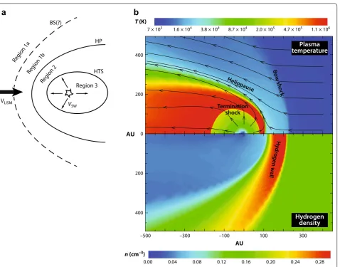
plasma environment is composed of essentially three thermodynamically distinct regions: (i) the supersonic solar wind, with a relatively low temperature, large radial speeds, and low densities, bounded by the heliospheric termination shock (HTS). The outer heliosphere is that region of the solar wind influenced dynamically by physi-cal processes associated with the LISM. (ii) The transition of the supersonic solar wind to a subsonic flow through the HTS creates a region of heated subsonic solar wind, called the inner heliosheath (IHS). The IHS has much higher temperatures and densities, larger magnetic fields, and lower flow speeds than does the distant supersonic solar wind (SW). The IHS is bounded by a contact or tan-gential discontinuity called the heliopause (HP). (iii) The HP is the boundary that separates plasma of solar ori-gin from plasma of interstellar oriori-gin. The LISM in our neighborhood possesses a small plasma flow speed and temperature, but the density is higher than in regions (i) and (ii). A bow shock may or may not exist ahead of the heliosphere due to the relative motion of the Sun and interstellar medium. The three regions are illustrated in Fig. 1 (left panel), where region 3 corresponds to the supersonic solar wind, region 2 to the hot inner heli-osheath, and the interstellar region is subdivided into region 1b between the HP and a possible bow shock/ wave, sometimes called the outer heliosheath (OHS), and region 1a beyond a bow shock or bow wave. Of course, as we discuss below, the plasma system is vastly more complicated than that of MHD and the plasma itself pos-sesses multiple components coupled via charge-exchange and/or collisional and collisionless processes, with asso-ciated transfer of charge, momentum, and energy, and thus thermodynamic coupling. Nonetheless, the zeroth-order distinction of thermodynamically distinct regions provides a useful intuitive guide to the underlying physics of the global solar wind–LISM interaction.

Each of the thermodynamically distinct regions is the source of a distinct population of hydrogen (H) atoms produced by charge exchange between the ambi-ent plasma and neutrals ambi-entering the region (Zank et al. 1996). These three distinct neutral H populations include the “splash” component produced in the fast or super-sonic solar wind, i.e., fast neutrals that acquire high radially outward speeds (∼400−750  km/s) with a

rela-tively small thermal spread, very hot neutrals produced in the inner heliosheath with comparatively high speeds (∼100 km/s) and a large thermal spread (which can

pro-duce ENAs with speeds even that exceed 100  km/s), and decelerated heated atoms originating in the outer heliosheath.

The charge-exchange mean free path (mfp) of neutral hydrogen atoms in the LISM (region 1) is approximately

∼100 AU (assuming a charge-exchange cross-section

σc = 5 ×10−15 cm2 and a total LISM number density of  0.2 cm−3

), in the IHS (region 2) ∼2500 AU for a

num-ber density of 0.005 cm−3

, and >200 AU in the supersonic

solar wind beyond 10 AU (region 3). With the excep-tion of the local interstellar medium region, the charge-exchange mfps are so large that they exceed the expected scale size of the boundary regions separating the helio-sphere and LISM. The interaction of the solar wind with the LISM therefore requires the modeling of plasmas and non-equilibrated H atom gas. Despite the very large charge-exchange mfps in both the supersonic solar wind and the boundary regions, the structure of the global heliosphere is determined in large part by the non-equil-ibrated coupling of neutral interstellar H to supersonic and subsonic solar wind plasma (Zank 1999; 2015; Zank et al. 2009; McComas et al. 2011). This makes the mod-eling of the solar wind interaction with the LISM very challenging. Nonetheless, despite these complications, the basic structure illustrated in the cartoon Fig. 1 (left) emerges from simulations that include the basic physics of the plasma–H charge-exchange coupling. An illustra-tive simulation of a 2D coupled model of the heliospheric interaction with the LISM is shown in Fig. 1 (right panel). The top plot shows the 2D plasma temperature distribu-tion, clearly identifying the three distinct regions and the overall topology and boundaries that can exist (together with a further sub-division of region 1 into pre- and post-bow shock regions 1a and 1b, respectively). The bottom plot illustrates the neutral H density distribution. A more extended summary that discusses the magnetic field observations in both the IHS and at the HP, together with associated references and related theoretical modeling, can be found in the review by Zank (2015).

The coupling of plasma and neutral H occurs through the creation of PUIs via charge exchange between the charged and neutral gases. Over suitably large distances, the neutral H and protons are fully equilibrated, both possessing the same temperature and velocity. Charge exchange in a fully equilibrated partially ionized plasma has no essential dynamical effect, with charge exchange effectively doing no more than relabeling protons and H atoms (assuming that the dominant neutral gas com-ponent is H atoms—in the LISM, this is a reasonable assumption, although He atoms are approximately 9  % of the neutral gas and the remaining heavy atom neu-tral gas is about 1 %). However, in regions 2 and 3, the interstellar H drift speed is different from the plasma flow velocity (∼20  km/s for H versus ∼100−750  km/s

for the plasma), and H originating from regions 3 and 2 that splashes back into the LISM has flow speeds rang-ing from ∼100−>400 km/s, which is quite different from

the ∼15−26  km/s speed of region 1. Thus, throughout

AU of the HP, there is a relative drift between the back-ground plasma and some H components. Depending on the specific environment, the neutral gas can be ionized by either solar photons (photoionization) or charged par-ticles (charge exchange, electron-impact ionization) and the new ions are accelerated almost instantaneously by the motional electric field of the plasma. The PUIs form a ring-beam distribution on the time scale of the inverse gyrofrequency and stream along the magnetic field while experiencing advection by the bulk plasma flow perpen-dicular to the mean magnetic field. Newly created PUIs drive a host of plasma instabilities, from fast magneto-sonic and Alfvénic waves, ion cyclotron waves, to lower

hybrid waves (e.g., Lee and Ip 1987; Cairns and Zank

2002; Gary and Madland 1988, see Gary 1991; Isenberg 1995; Zank 1999 for extensive summaries). PUIs expe-rience scattering and gradual isotropization by either ambient or self-generated low-frequency electromagnetic fluctuations in the plasma. Since the newly born ions are eventually isotropized, their bulk velocity is essentially that of the background plasma, i.e., they advect with the plasma flow and are then said to be “picked up” by the flowing plasma. The isotropized PUIs form a distinct suprathermal population of energetic ions (∼1 keV ener-gies in the supersonic SW, with a number density approx-imately 20  % of the solar wind number density in the vicinity of the HTS) in the plasma whose origin is either the interstellar medium when considering region 3 and 2 AU

T (K)

AU

n (cm–3₎

b

a

Hydrogen density 7 × 103

400

200

0

200

400

–500

0.00 0.04 0.08 0.12 0.16 0.20 0.24 0.28

–300 –100 100 300

1.6 × 104 _{3.8 × 10}4 _{8.7 × 10}4 _{2.0 × 10}5 _{4.7 × 10}5 _{1.1 × 10}6

Heliopaus e

Termination shock

Bo_w sh

oc_k

Hy

dr

og

en

w

all

Plasma temperature Region 1a

Region 1b

Region 2

Region 3 HTS

HP BS(?)

VLISM _V

SW

Fig. 1 Left Schematic of the solar wind–VLISM boundary regions that correspond to distinguishable thermodynamic regions, and which act as neutral H sources whose characteristics are clearly distinct (after Zank et al. 2009). HTS heliospheric termination shock, HP is heliopause, BS is bow shock, VSW denotes the radial solar wind flow speed, and VLISM the LISM flow velocity. Right A 2D steady-state, 2-shock heliosphere showing, top plot,

or the heliosphere when considering regions 2 and 1 (e.g., Holzer 1972; Lee and Ip 1987; Williams and Zank 1994, see Zank 1999, 2015 for an extensive review).

Consider now the three specific regions discussed above. PUIs are created in these regions and mediate the plasma properties. Although each region is mediated by PUIs, the origin of the PUI population in each is different in important ways.

Coulomb collisions are necessary to thermally equili-brate a background thermal plasma, such as the solar wind, and the PUI protons. In the case of the supersonic solar wind, (Isenberg 1986) argued that a multi-fluid model is necessary to describe a coupled solar wind– PUI plasma since neither proton nor electron collisions can equilibrate the PUI-mediated supersonic solar wind plasma (see Zank et al. 2014).

The inner heliosheath (IHS) is complicated by the microphysics of the HTS. The supersonic solar wind is decelerated on crossing the quasi-perpendicular HTS. The flow velocity is directed away from the radial direc-tion and is ∼100 km/s. The interplanetary magnetic field

remains approximately perpendicular to the plasma flow. Voyager 2 measured the downstream solar wind tem-perature to be in the range of ~120,000–180,000 K ∼16

eV (Richardson 2008; Richardson et  al. 2008), which was much less than predicted by simple MHD models. Instead, the thermal energy in the IHS is dominated by PUIs. There are two primary sources of PUIs in the inner heliosheath. The first is interstellar neutrals that drift across the HP and charge exchange with hot solar wind plasma. These newly created ions are picked up in the IHS plasma in the same way that ions are picked up in the supersonic solar wind. The characteristic energy for PUIs created in this manner is ∼50 eV or ∼6 ×105 K,

which is about five times hotter than the IHS solar wind protons. The second primary source is PUIs created in the supersonic solar wind and then convected across the HTS into the IHS. The PUIs convected to the HTS are either transmitted immediately across the HTS or are reflected before transmission (Zank et al. 1996). PUI reflection was predicted by Zank et al. (1996) to be the primary dissipation mechanism at the quasi-perpendic-ular HTS, with the thermal solar wind protons experi-encing comparatively little heating across the HTS. The transmitted PUIs downstream of the HTS have tem-peratures ∼9.75 ×106  K (∼0.84  keV) and the reflected

protons have a temperature of ∼7.7 ×107 K (∼6.6 keV)

(Zank et al. 2010). PUIs, whether transmitted, reflected, or injected, dominate the thermal energy of the IHS, despite being only some 20  % of the thermal subsonic solar wind number density at the HTS. The IHS pro-ton distribution function can be approximated by a 3- (Zank et al. 2010; Burrows et al. 2010) or 4-component

distribution function (Zirnstein et al. 2014), with a rela-tively cool thermal solar wind Maxwellian distribution and two or three superimposed PUI distributions. Such a decomposition of the IHS proton distribution func-tion can be exploited in modeling energetic neutral atom (ENA) spectra observed by the IBEX spacecraft at 1 AU (Desai et al. 2012; Zirnstein et al. 2014; Desai et al. 2014). Multiple proton populations were identified in the IHS and the very local interstellar medium, these being the various PUI populations described above and the ther-mal solar wind proton population (Zank et  al. 2010). Zank et  al. (2014) show that in the IHS neither proton nor electron collisions can equilibrate a PUI-thermal solar wind plasma in the subsonic solar wind or IHS on scales smaller than at least 10,000 AU, meaning that a multi-component plasma description that discriminates between PUIs and the subsonic solar wind plasma is necessary.

The interstellar plasma upwind of the heliopause is also mediated by energetic PUIs. It was noted (Zank et  al. 1996) that energetic neutral H created via charge exchange in the IHS and fast solar wind could “splash” back into the interstellar medium where they would experience a secondary charge exchange. The secondary charge exchange of hot and/or fast neutral H with cold (∼7500 K—McComas et  al. (2012, 2015); Schwadron

et  al. (2015); Bzowski et  al. (2015) LISM protons leads to the creation of a hot or suprathermal PUI population locally in region 1. The heating of the LISM in the neigh-borhood of the Sun has been discussed in detail (Zank et al. 2013), since this results in an increased sound speed with a concomitant weakening or even elimination of the bow shock (yielding instead a bow wave) (McComas et al. 2012). PUIs form a tenuous (np≃5 × 10−5 cm−3,

(Zirn-stein et al. 2014) suprathermal component in the plasma upwind of the HP that is not collisionally equilibrated in the LISM on scales smaller than at least 75 AU (Zank et al. 2014).

Review

Selected observations

The crossing of the HTS by Voyager 2 (V2) revealed an almost classical perpendicular shock structure (labeled TS-3) (Burlaga et al. 2008; Richardson et al. 2008), except that the observed average downstream proton plasma temperature was an order of magnitude smaller than pre-dicted by the MHD Rankine–Hugoniot conditions (Zank et al. 2009). The transmitted solar wind proton distribu-tion is a broadened/heated Maxwellian (with a somewhat flattened peak), and there is no evidence of reflected solar wind ions being transmitted downstream (Richardson et  al. 2008; Richardson 2008). Richardson et  al. (2008);

Richardson (2009) concluded that PUIs provide both

the primary shock dissipation mechanism and the bulk of the hot plasma downstream of the HTS, as predicted 12  years earlier by Zank et  al. (1996). The basic model (Zank et  al. 1996) for the microstructure of the HTS therefore appears to be supported by V2 observations. However, both the observed solar wind proton distribu-tion and a shock dissipadistribu-tion mechanism based on PUIs mean that the downstream proton distribution function is a (possibly complicated) function of the physics of the HTS. Zank et al. (2010) developed a basic model of a quasi-perpendicular HTS, mediated by PUIs, to derive the complete downstream proton distribution function in the IHS, determine the partitioning of energy between solar wind protons and PUIs, and infer the implications of the constructed IHS proton distribution function for the ENA spectral flux observed by IBEX.

Zank et  al. (2010) introduced a three-distribution approximation of the IHS proton distribution, compris-ing core solar wind protons, transmitted (without reflec-tion) PUIs, and reflected (and then transmitted) PUIs. Electrons are of course included too in the complete plasma model. The reflected PUI population results from the reflection of some upstream PUIs at the cross-shock electrostatic potential of the quasi-perpendicular HTS. Reflected PUIs are the primary dissipation mechanism at the HTS (Zank et al. 1996; Lipatov and Zank 1999; Bur-rows et al. 2010). Although the post-HTS PUI distribu-tion is likely highly complex, as a first approximadistribu-tion the solar wind proton distribution is a Maxwellian. Since the number of PUIs reflected is comparatively small, a simplifying assumption that the non-reflected PUI dis-tribution can be approximated by either a filled-shell or a Maxwellian distribution can be made (Zank et  al. 2010). The downstream PUI temperatures for the trans-mitted and reflected PUIs can be computed (Zank et al. 2010), allowing the partitioning of downstream thermal energy into transmitted solar wind protons, transmit-ted PUIs and reflectransmit-ted, and then transmittransmit-ted PUIs to be determined. The smoothed form of the constructed

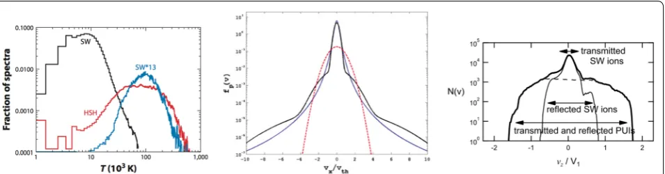
heliosheath proton distribution (Zank et al. 2010) resem-bles a κ-distribution (Heerikhuisen et  al. 2008). As a result, a significant number of protons reside in the wings of the distribution function, quite unlike the Maxwellian distribution. The close correspondence between the con-structed distributions and the κ-distribution with index 1.63 is useful in allowing for simplified simulations based on a κ-distribution (Heerikhuisen et al. 2008; Zank et al. 2010, 2013; Zank 2015). Zank et al. (2010) predicted that the constructed heliosheath proton distribution should possess some structure that would manifest itself in ENA spectra observed at 1 AU by IBEX, and that the micro-physics of the HTS plays a key role in determining the form of the total downstream or heliosheath proton dis-tribution. Finally, we note that kinetic hybrid and PIC simulations (Lipatov and Zank 1999; Oka et al. 2011; Wu et  al. 2009; Matsukiyo and Scholer (2011, (2014); Yang et al. 2015) appear to support the basic model (Zank et al. 1996, 2010) rather well. These comments are illustrated graphically in Fig. 2, where we show three panels. The left panel plots the solar wind proton distribution upstream and downstream of the HTS observed by the Voyager

2 plasma instrument PLS (Richardson 2008).

Unfortu-nately, the PLS instrument measures only solar wind energy protons and not PUIs. The observed downstream proton distribution shows clearly that the transmitted solar wind distribution is simply a heated Maxwellian distribution and no reflected solar wind protons can be identified. The middle panel shows the theoretically predicted total downstream proton velocity distribu-tion funcdistribu-tion Zank et al. (2010). The blue curve shows a κ-distribution with a kappa value of 1.63 (Heerikhuisen et al. 2008). The black curves depict the distribution con-structed from a superposition of transmitted solar wind protons, transmitted but not reflected PUIs, and reflected and then transmitted PUIs. The red curve illustrates a Maxwellian distribution for the observed downstream density and temperature. For this model, the heliosheath constructed proton distribution (black curve) assumed that downstream phase mixing of PUIs caused them to evolve into an approximately Maxwellian distribution. The assumption of a downstream PUI distribution inter-mediate to a filled shell and a Maxwellian distribution creates a shoulder feature in the total downstream proton distribution function (Zank et al. 2010). The right panel shows the total transmitted solar wind and PUI distri-bution function downstream of the HTS derived from a hybrid simulation (Oka et al. 2011)—see also Yang et al.

(2015)—assuming an upstream PUI number density of

theory introduced in Zank et al. (2010) to both Voyager 2 observations and simulations, the relative energies of downstream solar wind ions and transmitted (both directly and initially reflected) PUIs are clearly illustrated in Fig. 2.

To test the possibility that the microphysics of the HTS would manifest itself in IBEX ENA spectra observed at 1 AU, Desai et  al. (2012) in an initial study found that the fluxes, energy spectra, and energy dependence of

the spectral indices of ∼0.5–6  keV ENAs measured by

IBEX-Hi along the V1 and V2 lines of sight were consist-ent within a factor of ~2 with the model results of Zank et  al. (2010). The observed ENA spectra do not exhibit sharp cutoffs at approximately twice the solar wind speed as is typically found for shell-like PUI distributions in the heliosphere. Desai et al. concluded that the ENAs meas-ured by IBEX-Hi are generated by at least two types of PUI populations whose relative contributions depend on the ENA energy: transmitted PUIs in the ~0.5 to 5 keV energy range and reflected PUIs above ~5  keV energy (Desai et al. 2012).

The absence of sharp cutoffs in the ENA distribu-tion indicates that the ENA source in the ∼0.5–5  keV energy range is almost certainly beyond the HTS. The PUI distribution is modified by energization processes in the supersonic solar wind, such as the formation of the filled shell due to cooling, and it appears to develop an extended tail beyond v–2U (U the bulk solar wind speed). However, the tail does not emerge smoothly from the flat-topped PUI distribution function but instead appears as a discontinuous, lower intensity attachment

to the cutoff step at v∼2U of the filled shell distribution (see e.g., Gloeckler et al. 1994, 2001), and so a cutoff is still present. However, Gloeckler et al. (1994, 2001) show examples of the transmission of the solar wind PUI dis-tribution through a CIR reverse shock. The flat-topped PUI distribution is transformed into a kappa-like distri-bution on transmission through the interplanetary shock, i.e., a Maxwellian-like core with an extended tail that emerges smoothly from the thermal distribution. These observations, together with the theory described above, suggest that the observed ENAs are generated primarily downstream of the HTS, after the PUI distribution has been processed by the HTS, rather than upstream in the supersonic solar wind. A further interesting point con-cerns PUI, and hence ENA, energies higher than ∼6 keV. Since all upstream PUIs are processed by the HTS, this

produces PUIs in the ∼0.5–6  keV energy range

down-stream which do not have a flat-topped distribution. These energetic PUIs make up some 20  % of the pro-ton number density. Additional energization may result either at the shock (via, e.g., diffusive shock acceleration (Senanayake et  al. 2015) or further downstream (Zank et al. 2015), or deep in the IHS itself (Lazarian and Opher 2009; Fisk and Gloeckler 2009), and this would then lead to a modification of the total proton spectrum in the IHS. Although it is difficult to quantify the effect of additional proton energization in the IHS, if it produces a power law distribution from the energetic tail of the HTS-processed distribution, then this will simply ensure that (i) there is no cutoff at ∼6 keV; (ii) the intensity in the energy range ∼0.5–6 keV will be reduced a little (bearing in mind that

Fig. 2 Left histograms of the solar wind thermal proton temperature distributions observed by Voyager 2 across the HTS measured in the SW and IHS: (black) solar wind distribution, (red) IHS distribution, and (blue) distribution of the solar wind temperature multiplied by 13, the ratio between the upstream solar wind and downstream IHS temperatures. No reflected solar wind protons can be identified from the distribution function (Richardson 2008). Center the IHS constructed proton distribution (black curve) assuming that the transmitted but not reflected PUIs evolve into a Maxwellian distribution. The blue curve shows a κ-distribution with a value of −1.63. The black curve is the superposition of transmitted solar wind protons, transmitted PUIs, and reflected and then transmitted PUIs. The red curve is a Maxwellian distribution assuming the observed downstream density and temperature. The particle velocity vx is normalized to the Maxwellian thermal speed vth=

the new distribution is a power law), and (iii) this process is likely to be of more importance to higher energy ENA observations (such as the Cassini INCA observations of ENAs (Krimigis et al. 2009).

The observed lower energy ENAs (below ∼0.5  keV)

are not well described by the theory (Zank et al. 2010), and most existing models underestimate the ENA fluxes

between ∼0.05–0.5  keV by an order of magnitude or

more (Fuselier et al. 2012). To address the lower energies, Zirnstein et  al. (2014) extended the Zank et  al. (2010) model in two ways. First, they accounted for the extinc-tion of solar wind protons and transmitted and reflected PUIs by charge exchange with interstellar neutral H in the composite proton distribution. The extinction pro-cess alters the distribution of energy in the IHS, com-pared to assuming that the relative energy densities of the core SW protons and the transmitted and reflected PUIs remain constant. Determining an accurate partitioning of the energy is essential for understanding the role that PUIs play in the heliosphere and its effect on H ENA flux.

The second extension introduced by Zirnstein et  al.

(2014) was to include ENAs from the VLISM that were

created by PUIs. Although ENAs are created every-where in the solar wind–LISM interaction region, ENAs produced in the IHS easily propagate into the VLISM before charge exchange occurs, creating a population of PUIs there. ENAs produced in the VLISM, however, do not easily charge exchange in the IHS, and therefore permeate the inner heliosphere and can be detected

at 1 AU. One can similarly partition the VLISM energy into various proton populations (Zirnstein et  al. 2014). The VLISM plasma consists mostly of protons, initially ∼7500  K in the pristine LISM (McComas et  al. 2015; Schwadron et al. 2015; Bzowski et al. 2015), that are par-tially heated by charge exchange near the H wall and by crossing a bow wave (McComas et al. 2012; Zank et al.

2013). However, the increase in thermal energy of the

VLISM plasma near the HP is also due to energetic PUIs, which are created from charge exchange between LISM protons and ENAs from the IHS (Zank et al. 1996). The majority of PUIs are in close proximity to the HP and drop off exponentially at larger distances due to the mean free path of their parent ENAs, and due to advection with the LISM flow toward the HP (Zirnstein et al. 2014). As with the IHS, Zirnstein et  al. (2014) determine the VLISM PUI properties by partitioning the total energy from the plasma-neutral results between LISM protons and PUIs. Since ENAs from IHS protons may propa-gate into the VLISM and charge exchange to become PUIs, they treat the VLISM plasma as a five-component distribution, including protons from the core (and com-pressed) VLISM plasma, and PUIs created by charge exchange from IHS ENAs.

Figure 3a shows various sources of the H spectrum in the V1 and V2 direction based on an extended model (Zirn-stein et al. 2014) with a comparison to the corrected IBEX data (Desai et al. 2014). The results illustrated in Fig. 3 are based on a single set of parameters that were introduced

100

102

102

103

104

100 ₁₀1

ENA energy (keV) IBEX-Lo

IBEX-Hi

a

10–1

(ENAs/cm

2 s sr keV)

b

100

102

102

103

104

100 ₁₀1

ENA energy (keV) 10–1

(ENAs/cm

2 s sr keV) 2 OHS + 3 IHS

1 OHS + 3 IHS 3 IHS

Sec. ENAs OHS, ribbon 2 OHS

IBEX-Lo IBEX-Hi

in the model (Zirnstein et al. 2014). Specifically, Zirnstein et  al. (1) considered multiple possible sources for OHS PUIs whereas Desai et al. (2014) considered just one case for which the source of OHS PUIs was the IHS, and (2) explored different values for a heating parameter α in their simulations, whereas Desai et  al. (2014) assumed a fixed value α=1/4. The effect of varying these parameters was

discussed in detail by Zirnstein et al. (2014), and a simi-lar comparison of the theoretical model and IBEX obser-vations is presented in Fig. 4 of Zirnstein et al. (2014). As illustrated in Fig. 3, below ∼0.5 keV, the flux is dominated by ENAs from VLISM secondary PUIs, while ENAs from HTS transmitted and reflected PUIs dominate above 0.5  keV. Although a small fraction of ENAs from core solar wind protons are visible at 1 AU, most exit the HP and become PUIs in the VLISM, producing significant flux near ∼0.1 keV. Zirnstein et al. (2014) predict that a signif-icant part of the ENA flux seen at 1 AU comes from the VLISM. ENAs created from solar wind PUIs in the VLISM

dominate the flux below ∼0.2  keV, while

secondary-injected, secondary-transmitted, and secondary-reflected PUIs contribute a significant flux up to keV energies, com-parable to the flux from the IHS. Our current detailed model (Zirnstein et al. 2014) therefore exploits the proper-ties of PUIs that contribute to heating the VLISM plasma, thereby establishing that not only the low- but also the high-energy flux is a result of the coupling between the IHS and VLISM plasmas through charge exchange. PUIs from the IHS are the source of multiple PUI species in the VLISM. Simulation results (Zirnstein et al. 2014) compare favorably with IBEX data, although perhaps somewhat low at high energies compared to those observed by IBEX since VLISM PUIs created from supersonic solar wind ENAs, or time-dependent solar wind boundary conditions were not included. Nonetheless, these results suggest strong cou-pling between the IHS and VLISM plasmas through ENA

charge exchange, and VLISM PUIs up to ∼10  keV may

dominate the globally distributed ENA flux visible at 1 AU. The results from the theoretical models (Zank et al. 2010; Zirnstein et al. 2014) describing the interaction of the solar wind and the partially ionized LISM and the observational results (Desai et  al. 2012, 2014) confirm that indeed the IHS and VLISM are multi-component non-equilibrated plasmas. Simplified single-fluid MHD plasma descriptions do not capture the complexity of the plasma. The multi-component model introduced by Zank et al. (2014) is the first rigorous attempt to extend basic models to incorpo-rate the physics of non-thermal PUI distributions

Modeling a pickup ion‑mediated plasma

The outer heliosphere beyond the ionization cavity (i.e.,

≥ ∼8 AU) is dominated thermally by PUIs (e.g., Burlaga

et  al. 1994; Richardson et  al. 1995a; Zank 1999; 2015;

Zank et  al. 2014). As reported by Decker et  al. (2008,

2015), the inner heliosheath pressure contributed by

energetic PUIs and anomalous cosmic rays far exceeds that of the thermal background plasma and magnetic field. The VLISM can also be regarded as a multi-com-ponent plasma (Desai et  al. 2012, 2014; Zirnstein et  al. 2014).

Coulomb collisions can equilibrate a background ther-mal plasma and energetic protons. Assume that the back-ground thermal proton and electron distributions are Maxwellian. If we restrict our attention to PUIs, then they satisfy the ordering vts≪vp<vte, where vts/e denotes the

background proton/electron thermal speed respectively and vp the PUI speed. For PUIs experiencing scattering

off thermal protons and electrons from a Maxwellian dis-tribution function, the collision frequency between PUIs and protons and PUIs and electrons is given by

respectively. Here mp,e and np,e denote the proton and electron mass and number density, respectively, e the charge on an electron, Te the electron temperature, ε0 the

permittivity of free space, and ln the Coulomb loga-rithm. If the collisional time scale exceeds the character-istic flow time of the plasma region of interest, τf ≃L/U ,

where L is the size of the region and U the characteris-tic velocity, then the PUI distribution will not equilibrate

with the background thermal plasma. Expressions (1)

should be used to determine whether one needs to intro-duce a plasma model that distinguishes energetic PUIs from background or thermal plasma protons.

Zank et  al. (2014) present detailed estimates for the equilibration times for PUIs in the supersonic solar wind of the outer heliosphere, the subsonic solar wind (the inner heliosheath), and the VLSIM using appropri-ate plasma parameters. In all three regions, the plasma does not equilibrate and cannot therefore be described as a magnetized single-component plasma and at least some elements of a multi-component description are necessary.

PUIs drive streaming instabilities in one form or another, and experience pitch-angle scattering from both self-excited and pre-existing Alfvénic fluctuations. The initial PUI ring-beam distribution is scattered toward isotropy (Lee and Ip 1987; Williams and Zank 1994; Zank 1999; Cannon et  al. 2014). Besides pitch-angle scatter-ing by Alfvénic and magnetic field fluctuations, PUIs can experience diffusion in velocity space, both due to counter-propagating Alfvén waves and PUI excited lower hybrid waves, for example. As is typical, we assume that

(1) ν_sps= nse

4_ln�

2π ε02m2pv3

s−1, and ν_spe= nee

4_ln�m1/2

e 2(2π )3/2_ε2

pitch-angle scattering is the fastest process associated with wave-particle interactions and neglect velocity dif-fusion terms. As we show below, pitch-angle scattering serves to introduce both a collisionless heat flux and a non-isotropic pressure tensor into the transport equa-tions describing the PUIs. The pressure tensor modifica-tion is expressed as a collisionless viscosity tensor.

To describe a plasma that contains a non-equilibrated PUI population, we construct an appropriate multi-com-ponent plasma description for a thermal background plasma comprising electrons and protons and a non-equilibrated PUI component that is subject to pitch-angle scattering by turbulence and Alfvénic fluctuations. By making various approximations, we derive succes-sively simpler models. In so doing, we place on a more formal footing the derivation of the well-known two-fluid model of cosmic ray magnetohydrodynamics (Axford et  al. 1982; Webb 1983), showing, somewhat unexpect-edly and contrary to perceived wisdom, that the cosmic ray number density is in fact included implicitly in the total number density.

The multi‑component model

In deriving a multi-component plasma model that includes PUIs, we shall assume that the distribution func-tions for the background protons and electrons are each Maxwellian, which ensures the absence of heat flux or stress tensor terms for the background plasma. The exact continuity, momentum, and energy equations governing the thermal electrons (e) and protons (s) are therefore given by

Here ne,s, ue,s, and Pe,s are the macroscopic fluid variables for the electron/proton number density, velocity, and pressure, respectively, γe,s the electron/proton adiabatic

index, E the electric field, B the magnetic field, and qe,s

the charge of particle.

The streaming instability for the unstable PUI ring-beam distribution excites Alfvénic fluctuations. The self-generated fluctuations and in  situ turbu-lence serve to scatter PUIs in pitch-angle. The Alfvén waves and magnetic field fluctuations both propa-gate and convect with the bulk velocity of the system

(2) ∂ne,s

∂t + ∇ ·

ne,sue,s

=0;

(3) me,_pn_e,_p

∂u_e,s

∂t +

u_{e,s· ∇}u_e,s

= −∇Pe,_s+q_e,_sn_e,_sE+u_e,_s×B;

(4) ∂Pe,s

∂t +ue,s· ∇Pe,s+γe,sPe,s∇ ·ue,s=0.

U=U(u_e,u_s,u_p,ne,ns,np,me,mp), where np and up refer

to PUI variables. The PUIs are governed by the Boltz-mann transport equation with a collisional term δf/δt|c,

for average electric and magnetic fields E and B. On

transforming the transport equation (5) into a frame

that ensures there is no change in PUI momentum and energy due to scattering, assuming that the cross-helicity is zero, and introducing the random velocity c=v−U , we obtain

The velocity U is still unspecified so we choose U such

that E′_{≡E+U×B=0. This assumption corresponds}

to choosing

since we choose U�=0 (U is parallel to B and therefore arbitrary). The use of the velocity U then yields

By taking moments of (8), we can derive the evolution equations for the macroscopic PUI variables, such as

the number density np=

fd3c, momentum density

npu_pi=

cifd3c, and energy density. Moments of the collisional term δf/δt|c are zero. The zeroth moment of

(8) yields the continuity equation for PUIs,

where u_p is the PUI bulk velocity in the guiding center

frame. For the first moment, we multiply (8) by cj and integrate over velocity space. This yields, after a little algebra, the momentum equation for PUIs,

where εijk is the Levi-Civeta tensor. Note the presence of

the term

cicjfd3c, which is the momentum flux or pres-sure tensor.

(5) ∂f

∂t +v· ∇f + e mp

(E+v×B)· ∇_vf = δf δt c , (6) ∂f

∂t +(Ui+ci)

∂f

∂xi +

e mp

(E₊U_×B_)i+ e mp

(c_×B_)i

−∂Ui ∂t −

Uj+cj

∂Ui

∂xj

∂f

∂ci = δf

δt c . (7) U⊥=U−U�=

E×B B2 ≡U,

(8) ∂f

∂t +(Ui+ci)

∂f

∂xi +

e mp

(c_×B_)i

−∂Ui ∂t −

Uj+cj

∂Ui

∂xj

∂f

∂ci = δf

δt c . (9) ∂np

∂t + ∂ ∂xi

np

Ui+u_pi =0, (10) ∂ ∂t np

Uj+u_pj

+ ∇ ·

npU

Uj+u_pj

+npupUj

+ ∂

∂xi

cicjfd3c= e

To close Eq. (10), we need to evaluate the momentum flux, which requires that we solve (8) for the PUI distri-bution function f. In solving (8), we assume (1) that the PUI distribution is gyrotropic, and (2) that scattering of PUIs is sufficiently rapid to ensure that the PUI distribu-tion is nearly isotropic. We can therefore average (8) over gyrophase, obtaining the “focused transport equation” for non-relativistic particles (Isenberg 1997). Details of the derivation can be found in Ch. 5 of Zank (2014). To solve the gyrophase-averaged transport equation requires that we specify the scattering or collisional operator. We make the simplest possible choice, which is the isotropic pitch-angle diffusion operator,

where µ=cosθ is the cosine of the particle pitch-angle θ, and νs=τs−1 is the scattering frequency. The form of

the scattering operator (11) allows us to solve the focused transport equation using a Legendre polynomial expan-sion of the distribution function f. The second-order cor-rect solution to the gyrophase-averaged form of Eq. (8) is

where c= |c| is the particle random speed, b≡B/B is a

directional unit vector defined by the magnetic field, and

D/Dt ≡∂/∂t+Ui∂/∂xi is the convective derivative. The expansion terms f0, f1 and f2 are functions of position,

time, and particle random speed c, i.e., independent of

µ (and of course gyrophase φ). Of particular importance is the retention of the large-scale acceleration, and shear terms. These terms are often neglected in the derivation of the transport equation describing f0 (for relativistic

particles, the transport equation is the familiar cosmic ray transport equation). In deriving a multi-fluid model, retaining the various flow velocity terms is essential to derive the correct multi-fluid formulation for PUIs. We need to evaluate

(11) ∂

∂µ

νs(1−µ2) ∂f ∂µ

,

(12) f ≃f0+µf1+1

2(3µ 2

−1)f2;

(13) f0=f0(x,c,t);

(14) f1= − cτs

3 bi

∂f0

∂xi +DUi

Dt

τs 3bi

∂f0

∂c;

(15)

f2≃cτs 15

bibj

∂Uj ∂xi − 1 3 ∂Ui ∂xi ∂f0 ∂c,

cicjfd3c=

(ci−u_pi)(cj−u_pj)fd3c+npu_piu_pj

≡

c′_ic′_jfd3c+npu_piu_pj

≃

c′_ic′_j

f0+µf1+ 1

2(

3_µ2₋1_)f2

d3c′_+npu

piupj,

from which we find the zeroth- and first-order expressions,

Consequently, the first-order PUI stress tensor is identi-cally zero and the pressure is isotropic, δijPp.

The inclusion of the second-order terms yields a non-zero collisionless stress tensor. Since the PUI pressure is defined in the frame of the bulk PUI velocity u_p, the

dis-tribution function over which the integral is taken needs to be evaluated in this frame. Since the expression (15) for f2 is a function of the guiding center velocity U, we

need to transform to the frame U_p=U+u_p. On using the solution (15) for f2, we obtain

where the coefficient of viscosity η is defined as

The first equality in (20) is the formal definition of the coefficient of viscosity for the PUI gas. If we assume (probably reasonably) that |c| ≫ |u_p|, then we obtain the

second equality, which may be regarded as a PUI pressure moment weighted by the PUI scattering time. Finally, if we assume that τs is independent of c, we then obtain the

“classical” form (20) of the viscosity coefficient. The pres-sure tensor may therefore be expressed as

If we introduce a “viscosity matrix,”

(16)

c′_ic′_jf0d3c=

1

mp

δijPp

,

c_i′c′_jµf1d3c=0,

Pp≡mp4π 3

c′2f0c′

2

dc.

(17)

c′_x21 2(3µ

2

−1)f2d3c′=

c′_y21

2(3µ

2

−1)f2d3c′

= η 15

bibj

∂Upj ∂xi − 1 3 ∂Upi ∂xi ; (18)

c′_z21 2(3µ

2

−1)f2d3c′= −

2η 15

bibj

∂Upj ∂xi − 1 3 ∂Upi ∂xi ; (19)

c_i′c′_j1 2(3µ

2

−1)f2d3c′=0, (i�=j),

(20)

η≡ 4π

15

_∂

∂c′(c ′4

cτs)f0dc′≃ 4π

3

c′2τsf0c′ 2

dc′≃ Ppτs mp

.

(21)

�

Pij�=Pp�δij�+





1 0 0 0 1 0 0 0 ₋2



 η

15

� bkbℓ

∂Upk

∂xℓ −

1

3

∂Upm

∂xm

�

.

(22)

(Mkℓ)≡(ηkℓ)=

η

15bkbℓ

≃

₁

15

Ppτsbkbℓ mp

and note that ηij=ηji and η/15=η11+η22+η33=ηijδij

(since b2=1), we can rewrite (21) in the more revealing

“classical” stress tensor form,

The pressure tensor is therefore the sum of an isotropic scalar pressure Pp associated with drift and curvatur and

the stress tensor, i.e.,

The stress tensor is a generalization of the “classical” form in that several coefficients of viscosity are present, and of course the derivation here is for a collisionless charged gas of PUIs experiencing only pitch-angle scattering by turbulent magnetic fluctuations. Use of the pressure ten-sor (24) yields a “Navier-Stokes”-like modification of the PUI momentum equation,

where we used the transformation U_p=u_p+U for the remaining velocity terms in (10) and ρp=mpnp.

If we introduce c′_≡c−u

p as before, we can express

the heat flux q(x,t) through the definition

The equation for the total energy of the PUIs can then be derived from (8), yielding

(23) η

15

bkbℓ ∂Upk

∂xℓ − 1

3 ∂Upm

∂xm

= ηkℓ 2

∂Upk

∂xℓ + ∂Upℓ

∂xk

− 1 3ηkℓδkℓ

∂Upm ∂xm

= ηkℓ 2

_∂U

pk ∂xℓ +

∂Upℓ ∂xk

−2 3δkℓ

∂Upm ∂xm

. (24) � Pij �

=Pp � δij � +   1 0 0 0 1 0 0 0 −2

  ηkℓ 2 �_∂ Upk ∂xℓ

+∂Upℓ ∂xk

−2 3δkℓ

∂Upm ∂xm

�

≡PpI+�p.

(25) ∂

∂t �

ρ_pU_p�

+ ∇ ·�ρ_pU_pU_p+I_Pp� =enp

�

E₊U_p×B�

− ∇ · 

 1 0 0 0 1 0 0 0 −2



 η_kℓ

2 �_∂U

pk ∂xℓ

+∂Upℓ ∂xk

−2 3δkℓ

∂U_pm ∂xm

� ,

=enp �

E₊U_p×B�

− ∇ ·�_p

(26) qi(x,t)≡mp

₁

2c ′2_c′

ifd 3

c′= mp 2

c2cifd3c

−5

2upiPp− 1

2ρpu 2 pupi.

(27) ∂

∂t

₁

2ρpU 2 p+ 3 2Pp + ∂ ∂xi ₁

2ρpU 2 pUpi+

5

2PpUpi+�ijUpj+qi

=enpU_pi

Ei+U_p×B

i

,

after transforming to U_p. To evaluate the heat flux, we

have

and

In (28), we introduced the spatial diffusion coefficient

together with PUI speed-averaged form κ¯ij≡Kij. The

collisionless heat flux for PUIs is therefore described in terms of the PUi pressure gradient and consequently the averaged spatial diffusion introduces a PUI diffusion time and length scale into the multi-fluid system.

For continuous flows, the transport equation for the PUI pressure Pp can be derived from (27), yielding

illustrating that the PUI heat flux yields a spatial diffu-sion term in the PUI equation of state together with a viscous dissipation term. The PUI system of equations is properly closed and correct to the second-order. Note the typo in Zank et  al. (2014) since we mistakenly omitted the viscous term of Eq. (30) in the corresponding pres-sure equation.

The full system of PUI equations can be written in the form

which is the form we use below. 1

2

c′2c_i′f0d3c=π

c′3µbif0c′

2 dc′=0,

(28)

mp 2

c′2c′_iµf1d3c′= − 2_π

3 mp

c′2κij

∂f0

∂xj c′2dc′

= −1

2κ¯ij

∂Pp

∂xj

=qi(x,t).

(29)

κij≡bi c2_τ

s 3 bj,

(30) ∂Pp

∂t +Upi ∂Pp

∂xi +5

3Pp ∂U_pi

∂xi = 1

3 ∂ ∂xi

Kij

∂Pp ∂xj

−2

3�ij ∂U_pj

∂xi ,

(31) ∂ρ_p

∂t + ∇ ·

ρpUp

=0;

(32)

∂ ∂t

ρpUp

+ ∇ ·ρpUpUp+IPp+�

=enp

_E

+U_p×B

;

(33)

∂ ∂t

₁

2ρpU 2 p+

3

2Pp

+ ∇ ·

₁

2ρpU 2 pUp

+5

2Pp

U_p+�·U_p− 1

2

K_{· ∇Pp}

The full thermal electron–thermal proton–PUI multi-fluid system is therefore given by Eqs. (2)–(4) and (31)– (33) or (30), together with Maxwell’s equations,

where J is the current and µ0 the permeability of free

space. The diffusion tensor is assumed to be of a simple diagonal form (i.e., we do not include the off-diagonal terms associated with drift and curvature–see the discus-sion in Zank (2014) and we specify

We parametrize the perpendicular component of the heat conduction tensor by a term η <1. In estimating the diffusion coefficients (38) from (29), we choose a charac-teristic PUI speed for the region of interest and assume that the scattering time can be approximated by a time scale greater than the corresponding gyroperiod.

Single‑fluid‑like model

For many problems, the complete multi-component model derived above is far too complicated to solve. The multi-fluid system (2)–(4) and (31)–(33) or (30), together with Maxwell’s equations can be considerably reduced in complexity by making the key assumption that U_p≃u_s . The assumption that U_p≃u_s is quite reasonable since (i) the bulk flow velocity of the plasma is dominated by the background protons since the PUI component scat-ters off fluctuations moving with the background plasma speed and (ii) the large-scale motional electric field forces newly created PUIs to essentially co-move with the back-ground plasma flow perpendicular to the mean magnetic field. Accordingly, we let U_p≃u_s=U_i be the bulk pro-ton (i.e., thermal background propro-tons and PUIs) velocity. The thermal proton and PUI continuity and momentum equations are therefore trivially combined as

(34) ∂B

∂t = −∇ ×E;

(35)

∇ ×B=µ0J;

(36) ∇ ·B=0;

(37) J=e

nsus+npUp−neue

,

(38)

K= 



κ⊥ 0 0

0 κ⊥ 0

0 0 κ�



; κ_⊥=η

1

3�_pC

2 0, κ�=

1

3�_pC

2 0.

(39) ∂ni

∂t + ∇ ·(niUi)=0;

(40) mpni

∂U_i

∂t +Ui· ∇Ui

= −∇(Ps+Pp)

+eni(E+Ui×B)− ∇ ·�p,

where ni=ns+np. Since the PUIs are not thermally

equilibrated with the background plasma (Ts�=Tp), we

need to deal separately with the Ps and Pp equations.

These become

We can combine the proton Eqs. (39)–(42) with the elec-tron Eqs. (2)–(4) to obtain an MHD-like system of equa-tions. On defining the macroscopic variables,

we can express

where the smallness of the mass ratio ξ ≡me/mp≪1 has been exploited. Use of the approximations (44) allows us to combine the continuity and momentum equations in the usual way and to rewrite the thermal electron and proton pressure in terms of the single-fluid macroscopic variables. Thus,

where

Since we may assume that the current density is much less than the momentum flux, i.e., |J| ≪ |ρU|, we can simplify (48) further by neglecting the RHS. By assuming

(41) ∂Ps

∂t +Ui· ∇Ps+γsPs∇ ·Ui=0;

(42) ∂Pp

∂t +Ui ∂Pp

∂xi

+5

3Pp

∂Ui

∂xi

= 1

3

∂ ∂xi

Kij

∂Pp

∂xj

− 2

3�ij

∂Uj

∂xi .

(43) ρ≡mene+mpni; q≡ −e(ne−ni);

ρU_≡meneu_e+mpniU_i;J_{≡ −e(ne}u_e−niU_i),

(44) ne=

ρ−(mp/e)q mp(1−ξ )

≃ρ/mp; ni=

ρ+ξ(mp/e)q mp(1+ξ )

≃ρ/mp;

u_e=ρU−(mp/e)J

ρ−(mp/e)q

≃U−mp e

J

ρ; ui=

ρU+ξ(mp/e)J

ρ+ξ(mp/e)q ≃U,

(45) ∂ρ

∂t + ∇ ·(ρU)=0;

(46)

ρ

∂U

∂t +U· ∇U

= −∇(Pe+Ps+Pp)+J×B− ∇ ·�;

(47) ∂Ps

∂t +U· ∇Ps+γsPs∇ ·U=0;

(48) ∂Pe

∂t +U· ∇Pe+γePe∇ ·U= mp eρJ· ∇Pe+

γemp e Pe∇ ·

_J

ρ

,

�_kℓ= 

 1 0 0 0 1 0 0 0 −2



 η_kℓ

2 �

∂U_k ∂xℓ +

∂Uℓ ∂xk

−2 3δkℓ

∂Um ∂xm

that γe=γs=γ, we can combine the thermal proton and

electron equations in a single thermal plasma pressure equation with P≡Pe+Ps,

Note that at this point, no assumptions about either the thermal electron or proton pressures (or temperatures) have been made.

Finally, we need an equation for the electric field E . To do so, we multiply the respective momentum equa-tions by the electron or proton charge, sum, and use the approximations (44) to obtain

The generalized Ohm’s law is therefore

where we have retained the PUI pressure since in prin-ciple it can be a high-temperature component of the plasma system and ξPp may be comparable to the Pe

term. For typical cases of interest, however, the Pp term

can be neglected in Ohm’s law (50). Neglect of the elec-tron pressure and Hall current term then yields the usual form of Ohm’s law.

The reduced single-fluid model equations may there-fore be summarized as

The single-fluid description (51)–(55) differs from the standard MHD model in that a separate description for

(49) ∂P

∂t +U· ∇P+γP∇ ·U=0.

ξ

m_p

e

21

ρ

∂J ∂t + ∇ ·(

JU₊UJ₎

= mp eρ

∇Pe−J×B−ξ∇(Ps+Pp)

−ξ∇ ·�)+E₊U_×B.

(50) E= −U×B− mp

eρ

∇Pe−J×B−ξ∇Pp

,

(51) ∂ρ

∂t + ∇ ·(ρU)=0;

(52) ρ

∂U

∂t +U· ∇U

= −∇(P+Pp)+J×B− ∇ ·�;

(53)

∂ ∂t

₁

2ρU

2

+3

2(P+Pp)+ 1

2µ0B 2

+ ∇ ·

₁

2ρU

2_U

+5

2(P+Pp)U

+ 1 µ0

B2U₋ 1 µ0

U_·BB_+�·U_p−1

2K· ∇Pp

=0_;

(54) ∂P

∂t +U· ∇P+γP∇ ·U=0;

(55)

E= −U×B; ∂B

∂t = −∇ ×E; µ0J= ∇ ×B; ∇ ·B=0.

the PUI pressure is required. Instead of the conserva-tion of energy Eq. (53), one could use the PUI pressure Eq. (42) for continuous flows. PUIs introduce both a col-lisionless heat conduction and viscosity into the system.

The model Eqs. (51)–(55), despite being appropriate to non-relativistic PUIs, are identical to the so-called two-fluid MHD system of equations used to describe cosmic ray-mediated plasmas (Webb 1983). However, the deri-vation of the two models is substantially different in that the cosmic ray number density is explicitly neglected in the two-fluid cosmic ray model and a Chapman–Enskog derivation is not used in deriving the cosmic ray hydro-dynamic equations. Nonetheless, the sets of equations that emerge are the same indicating that the cosmic ray two-fluid equations do in fact include the cosmic ray number density explicitly.

The single-fluid-like model may be extended to include, e.g., anomalous cosmic rays (ACRs) as well as PUIs. In this case, the ACRs are relativistic particles. The same analysis carries over, and one has an obvious extension of the model Eqs. (51)–(55) with the inclusion of the ACR pressure. Thus, the extension of (51)–(55) is

where we have introduced the ACR pressure PA, the

corresponding stress tensor A, the ACR diffusion

ten-sor K_A and adiabatic index γA (4/3≤γA≤5/3). The

coupled system (56)–(61) is the simplest continuum

model to describe a non-equilibrated plasma compris-ing a thermal proton–electron plasma with suprathermal

(56) ∂ρ

∂t + ∇ ·(ρU)=0;

(57) ρ

∂U

∂t +U· ∇U

= −∇(P+Pp+PA)+J×B

− ∇ ·�p− ∇ ·�A;

(58) ∂P

∂t +U· ∇P+γP∇ ·U=0;

(59)

∂Pp

∂t +U· ∇Pp+γpPp∇ ·U

= 1

3∇ ·

Kp· ∇P_p

−(γp−1)�p:(∇U);

(60)

∂PA

∂t +U· ∇PA+γAPA∇ ·U

= 1

3∇ ·(KA· ∇PA)−(γA−1)�A:(∇U);

(61)

E= −U×B; ∂B

particles (e.g., PUIs or even solar energetic particles) and relativistic energy (anomalous) cosmic rays. The system includes both the collisionless heat flux and viscosity associated with the suprathermal and relativistic particle distributions.

On reverting to Eqs. (51)–(55), we can recover the standard form of the MHD equations if we set the heat conduction spatial diffusion tensor K=0 and the

coef-ficient of viscosity (ηkl)=0, which corresponds to

assuming τs→0. If the total thermodynamic pressure Ptotal=P+Pp is introduced, then we recover the

stand-ard MHD equations (dropping the subscript “total”), i.e.,

with an equation of state e=αnkBT/(γ −1). The choice

of α=2 (or greater if incorporating the contribution of cosmic rays, etc.) corresponds to a plasma population comprising protons and electrons.

In setting K=0 and (ηkl)=0, we have implicitly

assumed that PUIs are completely coupled to the thermal plasma. With K�=0, heat conduction reduces the

effec-tive coupling of energetic particles to the thermal plasma, and their contribution to the total pressure is not as large. This will have important consequences for numeri-cal models of, e.g., the large-snumeri-cale heliosphere since they incorporate PUIs into the MHD equations, without dis-tinguishing PUIs from thermal plasma and therefore neglect heat conduction. Consequently, the total pressure is over-estimated.

Conclusions

Observations by Voyager 1 and 2 and the IBEX spacecraft indicate that plasma in the outer heliosphere (the super- and subsonic solar wind) and the VLISM possesses characteristics of a multi-component plasma, being essentially a non-equilibrated distribution of background thermal protons and electrons and PUIs of various ori-gins. Limitations of space prevent discussion of all the observational threads that lead to this conclusion, and we list and discuss above only a few. In the supersonic solar

(62) ∂ρ

∂t + ∇ ·(ρU)=0;

(63)

ρ∂U

∂t +ρU· ∇U+(γ −1)∇e+(∇ ×B)×B=0;

(64)

∂ ∂t

₁

2ρU

2

+e+ B

2

2µ0

+ ∇ ·

₁

2ρU

2

+γe

U

+ 1

µ0

B_×(U_×B₎

=0;

(65) ∂B

∂t = ∇ ×(U×B); ∇ ·B=0,

wind region of the outer heliosphere, the anomalous heating of the solar wind (Williams et al. 1995) has been interpreted in terms of the dissipation of PUI-driven turbulence that leads to the heating of the solar wind plasma (Zank et  al. 1996; 2012; Matthaeus et  al. 1996, 1999; Smith et  al. 2001; Adhikari et  al. 2015a). In the inner heliosheath and the VLISM, the observed plasma characteristics of the HTS (Zank et al. 1996; Richardson 2008; Richardson et al. 2008) and the ENA observations made by IBEX (Zank et al. 2010; Desai et al. 2012, 2014; Zirnstein et al. 2014) have been similarly interpreted in terms of a multi-component plasma distribution com-prising various PUI populations. Estimates of the col-lisional frequency between thermal plasma components and PUIs in the outer supersonic solar wind (>∼10

AU), IHS, and VLISM show that equilibration cannot be achieved in these regions. Illustrated in Fig. 4 is a sche-matic of the solar wind–LISM interaction region with colors indicating regions that have to be described in terms of a multi-component plasma. The three colors for the different regions indicate that each region has a dis-tinct multi-component plasma description reflecting the different origins of the PUI population for each. In the

supersonic solar wind, it is primarily PUIs created from interstellar neutral H that make up the PUI component. In the IHS, PUIs created in the supersonic solar wind and processed by the HTS are the most important PUI com-ponent energetically in the IHS, although there is a lower number density PUI component due to charge exchange with interstellar H as well. For the VLISM, the PUIs arise from charge exchange with secondary “solar wind or splash component neutrals” that were created in the supersonic solar wind and IHS. Basic plasma properties are mediated by PUIs in each of the regions illustrated in Fig. 4, and some discussion of the linear wave modes in these regions was presented by Zank et al. (2014). Table 1 provides a precise breakdown of the plasma models that are necessary for each region, together with estimates of the corresponding plasma and PUI temperature and den-sity for each species (second column). Possible simplifica-tions of the full model are listed in the third column for the IHS case.

Having motivated the need for a multi-component plasma description throughout the solar wind–VLISM interaction region, a derivation of the multi-fluid plasma model was presented, based on the analysis of Zank et  al. (2014) (and correcting some typos). The stand-ard approach of simply using a set of multi-fluid equa-tions under the assumption that all distribuequa-tions are isotropic, as done by Zieger et al. (2015), is incorrect in that it neglects the basic physics of PUI scattering by pre-existing and self-excited fluctuations. Numerous observations of the flat-topped form of the PUI distribu-tion in the solar wind show that wave-particle scattering

is fundamental to the physics of PUIs—for a review, see Zank (1999). Wave-particle scattering of PUIs introduces a collisionless form of PUI heat conduction and viscosity through the PUI pressure tensor. These important dissi-pative terms need to be included in any description of a non-equilibrated PUI-mediated plasma. The model pre-sented here is appropriate for use in models of the global heliosphere. In particular, in the inner heliosheath, the role of PUI and ACR heat flux is to partially decouple the full pressure contribution of the PUIs and energetic parti-cles from the overall pressure, thereby reducing the effec-tive thermodynamic pressure balancing the interstellar pressure against that of the inner heliosheath. The net effect should be a thinner heliosheath than predicted by conventional MHD models that over-estimate the total pressure contribution contributed by energetic particles. The new model equations should be used to explore the global structure of the solar wind–VLISM interaction eventually (but this is well beyond the current scope of the paper). Finally, we note that it is not completely obvi-ous how or whether ENA fluxes would change. At lead-ing order, the energy densities of the different ionized components should be largely unchanged in the IHS. The only difference is that the heat flux associated with ener-getic particles removes energy (i.e., reduces their pres-sure contribution) from the overall total prespres-sure of the inner heliosheath. Because this could lead to a thinner heliosheath, the ENA flux could be reduced but because the heat flux causes the energetic ionized particles to dif-fuse to greater distances; the net effect may be that there is little change in the overall ENA fluxes.

Table 1 An explicit listing of the possible separate PUI populations for the different regions illustrated in Fig. 4

Characteristic temperatures and densities are given for the different PUI species. In estimating np for interstellar PUIs created in the IHS, we assumed a characteristic

time scale of 40 AU/100 km/s ∼6×107  _s

Region Plasma model Reduced model

<8 AU (within ionization

cavity) Standard MHD model—PUIs essentially treated as test particles ~8 AU to HTS (i.e., beyond

ionization cavity)

Multi-component model

Interstellar PUIs created in solar wind (T≤1 _keV, np∼0.05−0.2ni) + ther-mal plasma (protons and electrons)

IHS Multi-component model Three PUI populations:

1) Interstellar PUIs transmitted across HTS without reflection (T∼1 keV,

np∼0.18ni)

2) Interstellar PUIs reflected and then transmitted at HTS (T∼6 –7 keV, np∼0.02ni)

3) Interstellar PUIs created in IHS (T∼50 eV, np∼0.015ni) + thermal

plasma (T∼16 _eV, ni∼0.005 cm−3)

Multi-component model

1) Retain 1) + 2) and incorporate 3) in thermal plasma model (i.e., neglect heat flux for T∼50_{eV PUIs)}

2) Combine models 1) and 2) and incorpo-rate 3) in thermal plasma model

VLISM Multi-component model

Solar wind PUIs created in VLISM (T ∼200 _eV, np∼5×10− 5