R E S E A R C H A R T I C L E
Open Access
Space–time POD based
computational
vademecums
for parametric studies:
application to thermo-mechanical
problems
Y. Lu
*, N. Blal and A. Gravouil
*Correspondence: [email protected] CNRS UMR5259, INSA-Lyon, LaMCoS, Univ Lyon, Villeurbanne, France
Abstract
Standard numerical simulations for optimization or inverse identification of welding processes remain costly and difficult due to their multi-parametric aspect and inherent complexity. The aim of this paper is to propose a non-intrusive strategy for building
computational vademecumsdedicated to real-time simulations of nonlinear
thermo-mechanical problems. There is in essence, a set of precomputed space–time parametric solutions (snapshots), selected by an appropriate approach in the
parameter space and stored in memory as quasi-optimal reduced bases (RBs) provided by the proper orthogonal decomposition method. Once the RBs are obtained, the
computational vademecumscan be used online and provide real-time space–time transient nonlinear thermo-mechanical solutions for any desired parameter value. The contributions of the paper consist in a space–time RBs interpolation approach with the Grassmann manifolds method, and a localized multigrid selection method that allows an automatic selection of snapshots in the parameter areas of interest for a given level of accuracy. As application, the welding simulation is considered with a transient non-linear thermo-mechanical model using the finite element method. It is shown that the moving frame allows an optimal design of the RBs. A good efficiency of the proposed approach is demonstrated.Computational vademecumscan be used for optimization or inverse identification problems of welding.
Keywords: Computational vademecums, POD, localized multigrid selection, Grassmann manifold interpolation
Introduction
Despite the increasing computer efficiency over the last decades, numerical simulations of welding processes remain prohibitive in terms of CPU time and storage, due to their multi-parametric aspect. To estimate the welding quantities of interest (residual stress, distortion, etc.) depending on different input parameters (typically, the geometry, materi-als properties, boundary conditions and the imposed loading), larges computations have to be re-run. Thus, the construction ofcomputational vademecums[1] (called also
vir-©The Author(s) 2018. This article is distributed under the terms of the Creative Commons Attribution 4.0 International License (http://creativecommons.org/licenses/by/4.0/), which permits unrestricted use, distribution, and reproduction in any medium, provided you give appropriate credit to the original author(s) and the source, provide a link to the Creative Commons license, and indicate if changes were made.
tual charts [2,3] or meta-model computations) with standard computations remains a cumbersome task.
The idea of computational vademecums consists in computing at the offline stage general solutions of a parametric problem, so as to make available a database of solu-tions. Engineers can then use these vademecums at the online phase for design, opti-mization or identification, etc. Although the offline computation can be costly, it is advantageous to lose time at this stage compared to that earned at online phase, espe-cially in the case of repetitive tasks. This paper focuses on the construction of numer-ical vademecums and the reduction of the associated costs for a given level of accu-racy.
As mentioned earlier, the construction ofcomputational vademecumswith standard computations based on full order models for welding simulations is out of reach. It seems important to make use of reduced-order model (ROM) techniques in order to develop models with a minimal number of degrees of freedom.
Reduction methods consist in finding a reduced basis (RB){Λi}ki=1, with an expected
small value of k compared to the number of degrees of freedom of the finite element approximation or to the number of time steps, that spans the subspace of the original solution function X(x, t)
X(x, t)≈ k
i=1
λi(t)Λi(x) (1)
Generally speaking, methods for building RBs can be classified into two families: a posteriori approaches and a priori approaches. Either, RBs are built a posterior from snapshots in the parametric space, or a priori (on the fly) during the calculation of the meta-model. A posteriori approaches require prior solutions (the so-called snap-shots) precomputed with standard full models and the accuracy of online solutions depends strongly on the quality of RBs computed with snapshots. The proper orthog-onal decomposition (POD) method [4], also known as Principal Component Analysis (PCA) [5–7] and Karhunen–Loeve Transform (KLT) [8,9], is often employed to build the RBs. It is worthwhile to mention that the computed POD basis is optimal with respect to given measures. This preliminary phase is called the offline phaseand can be costly. Such approaches have been applied to tackle many different problems in sci-ences and engineering [10–15]. Their main drawback resides in their inefficiency when one deals with non-linear problems, since the full tangent stiffness matrix needs to be rebuilt.
Efficient ROMs lie usually on a mixed approach between a posteriori and a priori approaches. They consist of a reduction step based on POD and an enrichment stage in order to improve the quality of these RBs. Interested readers can be referred to [27] for an enrichment technique originally proposed by Ryckelynck. This approach is of success applied to solve complex fluid flows [28,29] and speeds up thermomechanical simulations [30,31].
Recently, Chinesta successfully extended the separated representation, i.e. PGD meth-ods, for solving parametric (and thus multi-dimensional) problems [16,32–34], by adding extra-coordinates, related to model parameters or boundary conditions, to standard space–time solutions, and developed a series of computational vademecumsmethods for different problems in sciences and engineering such as thermal control of industrial furnaces [35], shape optimization [36], computational surgery [37], etc. These results are very encouraging. The PGD methods make possible efficient simulations of complex high-dimensional problems and the resultingcomputational vademecumsthat give real-time responses open numerous possibilities in the context of simulation based engineering, e.g. optimization or inverse identification which is also at the heart of the construction of computational vademecumsfor welding.
Nevertheless, one relies on the a posteriori POD approaches, because preliminary computed snapshots are sometimes available and it is obviously advantageous to use them for constructing optimal RBs instead of leaving behind the previous knowledge. As encountered in nonlinear problems, recomputing the tangent matrix makes inefficient the standard POD approaches. Although several approaches, e.g. the Discrete Empirical Interpolation Method (DEIM) [38], the hyper-reduction methods [11,27] and the asymp-totic numerical method that allows eliminating the recomputation of the tangent matrix [4,39,40], are introduced to accelerate the computations, real time requirements remain intractable. In addition, RBs lack robustness with respect to the variation of parameter value when one deals with parametric problems. In the works of [31], a hyper-reduced model coupled with an interpolation technique [41] based on Grassmann manifolds has been applied for the adaptation of the space RBs to tackle the robustness issue. However computing of the remaining parts (generally the time RBs) is still time-consuming work.
This work presents a methodology to overcome the above issues that go with the a pos-teriori approaches for space–time nonlinear parametric problems. The space and time RBs are both adapted by intensive use of the Grassmann manifolds interpolation. The recomputing of stiffness tangent matrix online can be then avoided. Once the snapshots are computed offline, there is no computation anymore and thus real-time parametric responses at online phase can be expected both in space and time. Furthermore, this approach is not intrusive, which can make available existing industrial software for differ-ent problems.
on a localized “multi-grid” approach (in the parameter space), allowing a quasi-optimal computational vademecum(quasi-optimal RB for a given level of accuracy), that provides reliable solutions.
The purpose of the strategy is to construct a space–time (4 dimensional) “computational vademecums” with controlled error for welding problems. To this end, the concerned transient nonlinear thermo-mechanical problem is presented in “Thermo-mechanical formulation” section. A brief review of model reduction techniques is proposed in “Design of reduced basis” section. The adaptation approach dedicated to parametric studies is detailed in “ROM adaptation for parametric studies” section. An academic example of welding is studied in terms of reducibility aspect in “Reducibility of welding simulations” section. In “Quasi-optimal computational vademecums with error control-application to welding simulations” section the quasi-optimalcomputational vademecumsare built. Finally, This paper is closed by some remarks in “Conclusion” section.
Thermo-mechanical formulation
In this section, a standard Lagrange formulation for transient nonlinear thermo-elasto-plastic problems is presented. More particularly, an alternative formulation in the moving frame is considered. For the application in welding processes, a sequentially coupled thermo-mechanical analysis is performed. The temperature is assumed to be independent on the mechanical fields.
Thermal analysis
Let us consider a material domainΩof densityρ, specific heat capacityC, and conductiv-ity tensork, with an initial temperature fieldT0. The bodyΩis subjected to a heat source
r, a prescribed temperatureTover the subspace∂ΩTand a surface flux q on the comple-mentary subspace∂Ωq(∂Ω =∂Ωq∪∂ΩT). Denoting byθ =T −T0the difference of
temperature between the actual and initial states, the governing equations, boundary and initial conditions to be satisfied by the thermal problem read as follows:
⎧ ⎪ ⎪ ⎪ ⎪ ⎪ ⎪ ⎪ ⎪ ⎨ ⎪ ⎪ ⎪ ⎪ ⎪ ⎪ ⎪ ⎪ ⎩
ρCdθ(dtX,t)+divq(X, t)=r(X, t)
q(X, t)= −k· ∇θ(X, t)
q(X, t)·n(X, t)=q(X, t) on∂Ωq θ(X, t)=θ(X, t) on∂ΩT
θ(X, t=0)=0
(2)
where “div•” (resp. “∇ •”) is the divergence (resp. gradient) operator with respect to the initial positionXand d•/dt the material time derivative.
In order to improve the computational efficiency for processes with moving heat loading like welding, [46,47] have proposed to solve thermal problems in moving frame, where the heat flux is fixed in space and the material flows through a reference configuration. Indeed, it is shown that for welding problems the quasi-state transient thermal problem can be simplified to a steady-state problem in a such configuration [47].
given timet, the coordinatex(with respect to the material configuration) of a material point which occupied the initial positionXat initial time inΩcan be given by a smooth motion mappingf:
x=f(X, t) (3)
Hence, the material time derivative in the flowing body reads:
dθ(x, t) dt =
∂θ(x, t)
∂t +v.∇θ(x, t) (4)
where ∂θ(∂xt,t)represents the local temperature variation over time,v= ddtxis the velocity vector which depends on the mappingf andv.∇θ(x, t) is the advection term.
By replacing this derivative expression in the previous Eq. (2), the heat equation defined in the control volume ˜Ωis expressed as:
divq(x, t)+ρC∂θ(x, t)
∂t +ρCv.∇θ(x, t)=r(x, t) (5)
For steady-state processes, the local temperature variation over time in the control volume can be neglected [47], which yields to:
divq(x, t)+ρCv.∇θ(x, t)=r(x, t) with∂θ(x, t)
∂t =0 (6)
It should be notified that the solutions are solved in the control volume ˜Ω, where boundary conditions (BCs) are not defined and should be chosen in an appropriate way to approximate original solutions in the fixed frame. Recently, similar use of moving reference is proposed for thermal analysis within a computational framework ofVademecum-based GFEM [48]. In this method, boundary conditions of the control volume are not needed to impose, because they are treated as extra-coordinates and considered in general cases. But it is not the case of this paper.
Mechanical analysis
The mechanical analysis is carried in the fixed frame, although the thermal analysis can be performed in the moving frame. In this case, a reverse of change of variables is particularly used for obtaining the representation of thermal temperature in the fixed frame:
θ(X, t)=θ(f−1(x), t) (7)
Otherwise, special techniques such as streamline integration [49,50] must be employed for dealing with this problem.
For the mechanical problems, the displacement and transformation are small. Hence the governing equations are solved on the undeformed initial material configuration. Then, the infinitesimal strain tensor ε is linked to the displacement fieldu by the linearized relationship:
ε= ∇su(X, t) (8)
where∇sdenotes the symmetric gradient operator. The total strainεis the sum of elastic, plastic and thermal strains denoted byεe,εp,εθ respectively, and only the elastic strain contributes to the Cauchy stressσ, i.e.
whereDdenotes the fourth order elasticity tensor andεθ =αθI(Iis the second-order identity tensor) results from thermal expansion, (•:•) is the double-contracted product. Considering the domainΩ subjected to a body force fwith prescribed forcesF and displacement u on boundaries∂ΩF and∂Ωu respectively (∂Ω = ∂ΩF ∪∂Ωu), static elasto-plastic analysis consists in seeking the admissible fieldsσ,uandεpsatisfying the following balance equations and boundary conditions:
⎧ ⎪ ⎪ ⎨ ⎪ ⎪ ⎩
divσ(X, t)+f(X, t)=0
σ(X, t)·n(X, t)=F(X, t) on∂ΩF
u(X, t)=u(X, t) on∂Ωu
(10)
with a complementary plastic behavior law, e.g. the associativeJ2plasticity theory
incor-porated with an isotropic hardening R reads: ⎧
⎨ ⎩
f(σ,p)=σd −σy−R(p) ˙
εp=H(f)<σdR: ˙gσd>σσdd
(11)
whereσydenotes the initial yield stress,H(•) the Heaviside function,σdthe deviatoric stress tensor,Athe positive part of A, p the equivalent plastic strains andg= ddRp.
Weak formulation of the thermo-elasto-plastic problem
The principle of virtual work is employed to develop the weak forms of governing equa-tions and the boundary condiequa-tions. Denoting byH1(Ω) the variational first order Sobolev
space, the transient thermal problem defined in the fixed frame has the variational descrip-tion: ⎧ ⎪ ⎪ ⎪ ⎪ ⎪ ⎨ ⎪ ⎪ ⎪ ⎪ ⎪ ⎩
findθ ∈Θsuch that
ΩρCθθ˙ ∗dΩ+
Ω∇θ.k.∇θ∗dΩ+
∂Ωqqθ∗ds=Ωrθ∗dΩ ∀θ∗∈Θ0
with Θ=θ(X, t)|θ(X, t)∈H1(Ω),θ| ∂Ωθ =θ Θ0=
θ∗(X, t)|θ∗(X, t)∈H1(Ω),θ∗| ∂Ωθ =0
(12)
The transient thermal problem defined in the moving frame is expressed as:
⎧ ⎪ ⎪ ⎪ ⎪ ⎨ ⎪ ⎪ ⎪ ⎪ ⎩
findθ ∈Θ˜ such that
˜
ΩρC ∂θ
∂t +v.∇θ
θ∗dΩ˜ +˜
Ω∇θ.k.∇θ∗dΩ˜ +
∂Ω˜qqθ∗ds=
˜
Ωrθ∗dΩ˜ ∀θ∗∈Θ˜0
with Θ˜ =
θ(x, t)|θ(x, t)∈H1( ˜Ω),θ|∂Ω˜θ =θ˜
˜ Θ0=
θ∗(x, t)|θ∗(x, t)∈H1( ˜Ω),θ∗| ∂Ω˜θ =0
(13)
In the same way, the steady-state problem formulation is obtained by neglecting the variation of temperature, i.e.∂θ∂t =0:
˜
ΩρCv.∇θθ
∗dΩ˜ +
˜
Ω∇θ.k.∇θ
∗dΩ˜ +
∂Ω˜qqθ
∗ds=
˜ Ωrθ
⎧ ⎪ ⎪ ⎪ ⎪ ⎪ ⎨ ⎪ ⎪ ⎪ ⎪ ⎪ ⎩
findu∈U such that
−Ωσ(u) :ε(u∗)dΩ+Ωf.u∗dΩ+∂ΩFF¯.u∗ds=0 ∀u∗∈U0
with u∈U, U =u(X, t)|u(X, t)∈H1(Ω),u|∂Ωu =u
U0=
u∗(X, t)|u∗(X, t)∈H1(Ω),u∗|
∂Ωu =0
(15)
Finite element semi-discretized formulation
For numerical implementation, the spaceH1(Ω) is replaced by finite dimensional sub-space (subsub-space of shape function). The semi-discretized problem associated to the tran-sient heat load reads:
Kthθ(t)+Cθ˙(t)=Q(t) (16) whereKthandCare the usual thermal conductivity and capacity matrices,θandQare respectively the nodal temperature and external flux vector.
In the moving frame configuration, the semi-discretized equation has a similar form: ˜
Kthθ˜(t)+C˜θ˙˜(t)=Q˜(t) (17) where ˜(•) denotes the quantity defined in the control volume ˜Ω. The difference from the usual thermal conductivity matrix in (16) consists in a modified thermal conductivity matrix with an additive advection term:
˜
Kth=
elements
(BTthkBth+NTρCvTBth) (18)
where the Bth andNare the usual matrices respectively for temperature gradient and interpolation of the element temperatureθ.
The mechanical solutions are given when the following residual vanishes: ⎧ ⎪ ⎪ ⎨ ⎪ ⎪ ⎩
R(U(t))=Fext(U(t))−Fint(U(t))
with Fext(t)=ΩNTfdΩ+∂ΩFNTF¯ds Fint(t)=
ΩBTm.σdΩ
(19)
where Uis the nodal displacement vector,Fext andFint are respectively the associated external and internal force vectors.Bmis the usual matrix for displacement gradient.
This residual problem can be solved with the Newton–Raphson scheme and incorpo-rated with the radial return mapping algorithm for plasticity flows. The transient thermal problem is solved by a first order time integrator.
State vector of the thermo-mechanical problem
The state vector corresponds to the minimal vector needed for storing the space–time history of all the thermal and mechanical fields. It is the only data vector one keeps at the end of the FE computations. The necessary memory for the storage completely depends on the size of X. Therefore, the state vector should be chosen so that its size is as small as possible.
For the transient thermo-elasto-plastic problem, the state vector can be defined as:
X(X, t)=θ,U,εp,σ,p T (20) An alternative state vector when the thermal analysis is performed in moving frame reads:
X(X, t)=θ˜,U,εp,σ,p T
Moreover, the state variables are represented in an approximate way with the compres-sion tools. The concerning model reduction methods and space–time separated variable representation are presented in the next section.
Design of reduced basis
This section presents the generation of the reduced basis (RB) using the popular POD method. Among the various techniques for obtaining a reduced basis, POD constructs a RB that is optimal in the sense that a certain approximation error concerning the snapshots is minimized. Thus, the space spanned by the basis from POD often gives an excellent low-dimensional approximation.
Snapshot proper orthogonal decomposition
Given a set of snapshots X= {X(t1), ...,X(tm)} ∈Rn×m, the POD method seeks an orthog-onal projectorΠΦ,Φ=ΦΦTthat minimizes the summed projection error:
argmin Ψ ΨTΨ=I
m
i=1
X(ti)−ΠΨ,ΨX(ti)22 (22)
It can be proved that the solution of the previous minimization problem can be provided by the Singular Value Decomposition (SVD) of the space–time snapshot X:
X=ΦVT (23)
whereΦ=[Φ(1),. . .,Φ(n)]∈Rn×nandV=[V(1),. . .,V(m)]∈Rm×mare orthogonal and respectively the so-called space and time bases. And∈Rn×mcontains positive singular valuesσi(withi≤r = min(n, m)) in decreasing amplitudes. Then the optimal solution of (22) isΦK = {Φ(i)}|i=1,...,k (withk ≤ r). The minimum 2-norm error [51] from the approximated snapshots using the POD basis is then given by:
X−ΠΦK,ΦKXF = r
i=k+1σ 2
i (24)
where • Fdenotes the Frobenius norm.
Generally,k is chosen in such a way that a great compression is gained as far as the amount of the RB to store is concerned and the corresponding low rank approximation is sufficiently accurate. One adopts the following definition:
Definition 1 k-compressibility
A space–time field is said to bek-compressibleif the number of the space–time modes needed to obtain the solution within a given tolerance isk.
ROM adaptation for parametric studies
Reduced bases often lack robustness with respect to parameter variations and updating of snapshots. This section tackles the actualization of the RB for parametric studies. A local interpolation strategy based on the Grassmann manifolds interpolation is presented and will be applied in our case to the adaptation of both the space and time RBs.
Grassmann manifolds interpolation
Let Y0 ∈ Rp×k, wherek ≤ p, denote a full-rank orthogonal matrix associated with a
ST(k, p) , which is defined as the set of allp×korthonormal matrices. Besides, the columns ofY0form a basis of the subspaceS0of dimensionkinRp. This subspaceS0belongs to
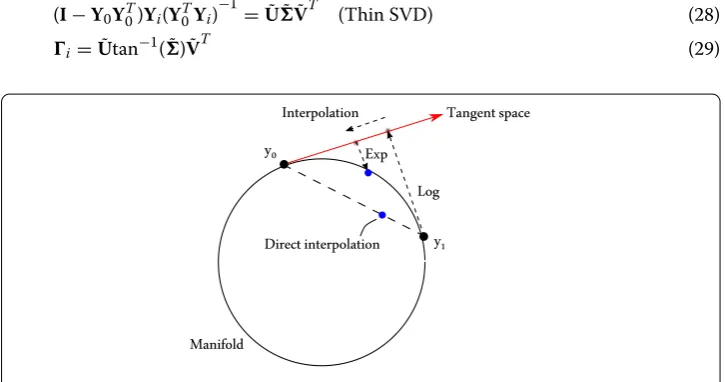
the Grassmann manifold [52,53]G(k, p) which is defined as the set of all k-dimensional subspaces ofRp. Generally, each k-dimensional subspaceScan be viewed as a point of G(k, p) at which there exists a tangent space of the same dimension [52,53]. This tangent space, denoted byT, is a “flat” space in which interpolation can be performed as usual [41] and can be represented by a matrix ∈Rp×k.
Lety(t) be a geodesic path uniquely defined by its initial and final pointsy0, y1∈G(k, p)
or initial point and velocityy(0)=y0,y˙(0)=y˙0∈T, the exponential mapping is defined as
the final extremity point, which maps a tangent space to the manifold itselfG(k, p)[52,54]:
Expy0(˙y0)=y(1)=y1 (25)
The inverse map, known as the logarithmic map, permits the back mapping from a point of the manifold to the tangent space.
Logy0(y1)=y˙0 (26)
Different analytic formulas for exponential and logarithmic mappings of matrix man-ifolds can be found in [55]. Coupled with a standard interpolation in the tangent space, exponential and logarithmic mappings allow defining a manifold-based interpolation (Fig.1).
In the case of Grassmann manifold, a computational framework for this interpolation has been proposed in [41]. Given a set of RBsYi|i=0,n∈Rp×kprecomputed at different oper-ating pointsSi|i=0,n(corresponding to different parameter valuessi|i=0,n), the geodesic of the Grassmann manifold, to which the subspaceSispanned by the RBs belong, can be described by the following equation [52,56]:
¨
Y+Y(YTY)−1Y˙TY˙=0 with YTY=I (27) In the same manifold, the following procedure permits the adaptation of the available RBs to a new operating pointSfor a valuesdifferent fromsi.
LetS0be the origin point, the tangent space spanned by the columns of iat this point is given by the logarithmic map [57]:
(I−Y0YT0)Yi(YT0Yi)−1=U˜˜V˜T (Thin SVD) (28) i=U˜tan−1( ˜) ˜VT (29)
The usual interpolation in this plane is then performed by calculating the FE basisNiin the parameter space:
Ni =
i=j s−sj si−sj
(30)
N = n
i=0
Ni i (31)
where N can be viewed as the mapping point ofS in the tangent space havingS0as
origin point. Herein a special case of 1D FE interpolation is presented. The application to 2 or 3 dimensional parameter cases is straightforward. More generally, a multivariate interpolation scheme (e.g [58,59]) can be used for multi-parameter cases.
The exponential map returns the adapted RB, which reads:
N =U˜N˜NV˜TN (Thin SVD) (32)
Y(s)=Y0V˜Ncos( ˜N)+U˜Nsin( ˜N) ˜
VTN (33)
where ˜VTN appears to guaranty the homogeneity of unity. In standard POD-Garlerkin models, the homogeneity for the interpolated basis is often abandoned (e.g [31,41]), since:
y(s)=spanY0V˜Ncos( ˜N)+U˜Nsin( ˜N)
(34)
In those models, only the space RB is interpolated for adaptation of the solution subspace, the homogeneity can be therefore abandoned. The loss of homogeneity is compensated by solving the equilibrium equation with FE computations when computing the remaining part (usually the time RB). Herein, keeping the homogeneity of interpolated bases is a crucial point and should be respected, since there is no resolution of equilibrium equa-tion for computing the time RB in the proposed method (both space and time RBs are interpolated in the Grassmann manifold).
A simplified form is obtained when there are only two RBs that are taken into account. Equations from (29) to (32) can be reduced to one equation:
Y(s)=
Y0V˜cos
s−s0
s1−s0
tan−1( ˜)
+U˜sin
s−s0
s1−s0
tan−1( ˜)
˜
VT (35)
Finally, It should be mentioned that the above computational framework is a special case of one varied parameter. We refer the readers to [41,52] for more details about the general case.
Space–time bases adaptation
Given two space–time solutions X0(X, t) and X1(X, t) pre-computed for two different
parameter valuesμ0andμ1respectively, then the POD basis is provided by SVD:
X0=Φ00VT0 (36)
X1=Φ11VT1 (37)
where the space and time bases are respectively Φi|i=0,1 and Vi|i=0,1. The new basis
{Φ(μ),V(μ)}corresponding to a new parameter valueμ∈[μ0,μ1] can be both obtained
by interpolations using the previous Grassmann manifolds interpolation method (see Algorithm 1). As mentioned before, homogeneity of unity with respect to Φi|i=0,1 and Vi|i=0,1should be kept here when interpolating the new basisΦ(μ) andV(μ) , otherwise
The singular value matrix (μ) can be directly interpolated with FE method, which yields to
(μ)= i
Ni(μ)i (38)
withNi(μ) is the FE basis in the parameter space.
Finally, the new solution X(X, t) corresponding to the new parameter valueμcan be then obtained by the combination of the interpolated matrices:
X=Φ(μ)(μ)VT(μ) (39)
Remark 1 Contrary to standard POD-Galerkin models, the proposed approach does not require new transient nonlinear FE computations with respect to the new parameter value. The space and time bases are both interpolated using Grassmann manifold inter-polation, which signifies that the variables homogeneity must be retained throughout interpolations. It can be highlighted that this interpolation-based procedure presents high efficiency in terms of time-cost. This provides a practical framework for parametric studies with low cost time computations as it will be shown hereinafter, even for transient nonlinear problems.
Remark 2 Application of the proposed approach to a 2D/3D parametric case can be simply carried out by employing the corresponding FE basis in Eqs. (31) and (38) for interpolation.
Remark 3 Due to the nature of the manifold-based interpolation, the solution rebuilt with this approach presents a notably better accuracy compared to a space–time adaptation with standard Lagrange interpolation methods. This point will be illustrated in the next part.
Local interpolation strategy
The space–time adaptation of the RB highly depends on the generated snapshots in the parameter space. In order to pre-compute the snapshots with a small number of trial points and a high fidelity, a local controlled error strategy is developed. Considering a transient nonlinear thermo-mechanical problem, the prior known solutions, correspond-ing to different parameter valuesμi=1,n∈[μ1,μn], are pre-computed with full FE method.
The POD snapshotsΦi,i,Viare provided by the truncated SVD method according to a k-compressibility criterion.
Note that while the local interpolation is performed for the space and time bases, the singular value matrix can be interpolated globally, i.e.
=
n
i=1 i=j μ−μj μi−μj
Remark 4 Though a global interpolation can indeed improve the accuracy of the rebuilt solution, the space and time bases are interpolated locally in view of the numerical cost increasing in the online phase and for the interpolation scheme stabilization.
Comparison with traditional interpolation methods
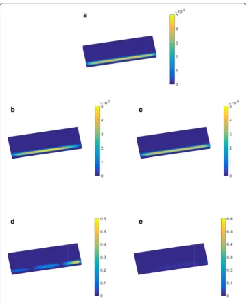
In order to show the efficiency of the proposed interpolation method, two examples of comparison are depicted in this section. As the first example, the comparison is performed between traditional methods and the proposed method for interpolating the seperated RBs. With two snapshots appropriately drawn in a 1D parameter space, the resulting equivalent plastic strain fields (recombined with the interpolated RBs) are illustrated in Fig.2. Compared with that obtained from full FE computations, the proposed approach can provide a good approximation (with a standard 2-norm error less than 1%). However, the Lagrange interpolation fails to interpolate RBs for new parameter values, the resulting solution shows a global error about 17%. Indeed, the RBs interpolated with traditional interpolation methods loss orthogonality (which should be guaranteed for POD-bases), while this property can be kept when using the proposed manifold-based interpolation.
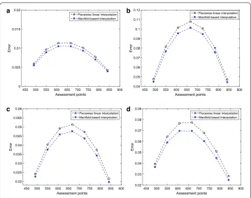
The second example consists in comparing the Grassmann interpolation with tradi-tional methods that interpolate straightforwardly solutions stemming form FE computa-tions (direct interpolation of snapshots). Given two snapshots calculated for two extremity values in the parameter space of thermal capacityμ:Cp∈[432,900]
J·kg−1·K−1(see Fig.3), the state variables are then interpolated for seven selected intermediate parameter values (called assessment points) using two different methods: piecewise linear interpo-lation and proposed manifold-based interpointerpo-lation. Figure4depicts the standard 2-norm error at assessment points for both thermal and mechanical variables interpolated with these two methods. It shows that the proposed manifold-based method improves more or less the quality of interpolated solutions both in thermal and mechanical cases with respect to piecewise linear interpolation. This can be explained by the fact that the pro-posed method takes into account the evolution of solutions at different time which may improve the interpolation accuracy. In addition, the proposed approach seems more suit-able for nonlinear cases. As shown in Fig.4, for the thermal problem, the proposed method improves only slightly the precision, while remarkable improvement can be observed in mechanical cases.
This confirms the efficiency of the proposed method with respect to the traditional interpolation methods, when only two snapshots are given. The comparison for higher order cases with more snapshots points in the parameter space is not taken into account here, since only local interpolation strategy is considered in our cases (see Algorithm 2).
Remark 5For the stability of methods, the space and time bases are interpolated mode by mode in the above examples.
Reducibility of welding simulations
Fig. 2 Equivalent plastic strain field comparisons [reference calculations (a) and online Lagrange (bandd) and Grassmann (cande) interpolation].aSolution from full FE computations.bSolution rebuilt by RBs interpolated with the Lagrange interpolation.cSolution rebuilt by RBs interpolated with the proposed method.dLocal error resulted from RBs interpolated with the Lagrange interpolation.eLocal error resulted from RBs interpolated with the proposed method
a b
d c
Fig. 4 Interpolation error for some assessment points in the parameter space (traditional piecewise linear interpolation vs proposed manifold-based interpolation).aError of temperature field.bError of displacemen field.cError of stress field.dError of plastic strain field
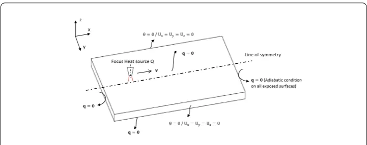
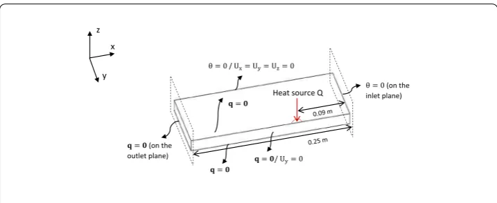
Welding finite element model
The work-piece with prescribed boundary conditions is shown in Fig.5. The heat source moves along the line of symmetry. The used material properties as well as the load param-eters are given in Table1. All the material properties are assumed independent on the temperature.
Since the problem (geometry, material, loading, BCs) is x–z plane symmetric, only one half of the actual problem is modeled Fig.6a. The mesh characteristics are presented in Table2.
Fig. 5 Welding work-piece: geometry and boundary conditions
Table 1 Material properties and load data
Notation Name Values
Cp Specific heat capacity 432 J·kg−1·K−1
λ Thermal conductivity 46 W·m−1·K−1
α Thermal expansion 1.2×10⁻⁵K−1
E Young’s modulus 210×109Pa
ν Poisson ratio 0.3
σy Initial yield stress 300×106Pa
H Linear isotropic hardening parameter 21×109Pa
Q Heat flux 8×10⁶W·m−2
V Velocity of loading 0.001 m·s−1
a b
Fig. 6 Problem definition with boundary conditions.aHalf model.bFE mesh
Table 2 Geometry parameter of FE model
Lx(m) Ly(m) Lz(m) E.T. E.N. N.N. G.N.
0.3 0.1 0.02 CUB8 (P1) 7200 9317 8
E.T.element type,E.N.element number,N.N.node number,G.N.Gauss point number per element
is prescribed with the initial temperatureθ0=0, while the outlet boundary is prescribed
with zero heat flux. The relation between the initial position of a material point and its actual position (3) can be written as:
Fig. 7 Control volume with boundary conditions
Reducibility of problem
The investigation of the problem reducibility is performed for the components of the state vector X defined in the previous section with a SVD analysis. For comparison purpose, the thermal solution (i.e.θor ˜θ) is solved in both the fixed and moving frames. In the sequel, the following definitions are used:
Definition 2 Relative SVD error
According to the Eckart–Young’s theorem [51], a relative error between the snapshot matrix X and the truncated SVD ˆX accountingkmodes is given by:
εk(X)=
X−Xˆ F XF =
X−ΠΦK,ΦKXF
XF =
r i=k+1σi2 r
i=1σi2
(42)
Definition 3 Energy SVD error estimator
A global space–time energy estimatorEkcan be defined for a state vector X (or one field of this state vector) through an integration over the time interval of a space-norm of X, e.g:
⎧ ⎨ ⎩
Ek( ˆU)= 12 T
0 uˆ(t).uˆ(t)dt= 12
k i=1σi2 Ek( ˆU)= EEtotk =1−ε
2
k
(43)
where ˆUdesignates a low rank approximation for the displacement fieldU ∈Rn×m,Ek defines a cumulative associated energy withkmodes andEk denotes a energy indicator with respect to the total associated energyEtotwhich is equal to 1 whenk=r=min(n, m).
Definition 4 Reducibility condition
In this analysis, a field is assumed to be reducible if the number of needed modes for its k-compressibility is less than 20% of the total number of modesr, i.e.kr <20%.
a
c b
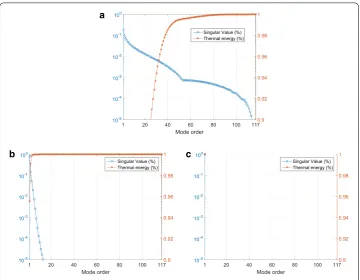
Fig. 8 Modes contribution forθ(top) and ˜θ(bottom).aTransient state solution in the fixed frame.
bTransient state solution in the moving frame.cSteady state solution in the moving frame
a b
d c
Fig. 9 Modes contribution for mechanical variables.aModes contribution forU.bModes contribution forσ.
thermal problem is significantly improved in the moving frame, since the thermal field is 3-compressible whereas it is 50-compressible in the fixed frame. Figure9 illustrates the application of SVD analysis to the mechanical problem solved in the fixed frame. A truncation energy of 99.99% requires less than 30 modes for each of these mechanical state variables, which makes the reducibility condition be satisfied.
The moving load and flowing heat flux induce the non-reducibility of the thermal prob-lem in the fixed frame. Whereas the resolution in the moving frame, which makes the moving load be fixed in reference configuration, leads to an hyper-reducible model. Fur-thermore, only one mode left with steady state assumption is required in our case. Contrary to the thermal problem, the mechanical problem is reducible in the fixed frame. Indeed, the mechanical field does not diffuse and is located in the domain of laser torch, while this is not the case for the temperature field that diffuses over time.
Thus, in order to guaranty the optimality of the RBs in the construction ofcomputational vademecumsof this welding model, the thermal problem is solved independently with a steady-state assumption in the moving frame. The mechanical problem is solved in the fixed frame. Finally, the state vector X is chosen as:
X=θ˜,U,εp,σ,p T
(44)
Quasi-optimalcomputational vademecumswith error control-application to welding simulations
This section tackles the precision problem of computational vademecums. A multi-grid based method is proposed to control the error produced in the construction of computational vademecums by Grassmann manifolds interpolation. Finally, the computational vademecums with error control are built based on the above welding model. In the following, the considered error is measured with respect to High Fidelity FE Models (HFM) and model discretization errors are not taken into account [44].
Reduced basis error indicator
Given XROM ∈Rn×mrebuilt with the approach proposed in “ROM adaptation for
para-metric studies” section, a reduced basis error indicator with respect to HFM is then defined as:
(X)= XROM(tm)−XHFM(tm)2 XHFM(tm)2
(45)
where (•)(tm) denotes the solution at the final time step and XHFMthe solution computed
with HFM.
Localized multigrid selection method
It is clear that an exhaustive generation of snapshots in the parameter space can ensure a reliable solution rebuilt by interpolation. However, the resulting offline time-cost is too much expensive. Herein, an efficient multigrid selection method that allows local refinements in the parameter space is presented.
Fig. 10 Successive localized refinements for a 2D parameter space
4D⊗1D thermalcomputational vademecum
An application of the proposed method to constructcomputational vademecumsis pre-sented herein. The notation 4D⊗1D means that solutions provided by thevademecums is 4D (in physical space: Ω ×[0tm]) and the concerned parameter space is 1D. Para-metric studies are performed with respect to the thermal capacityCp(J·kg−1·K−1) ∈
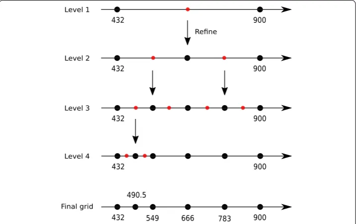
Fig. 11 Localized multigrid refinement in the 1D parameter space: the final sampling points obtained by the final grid are{432,490.5,549,666,783,900}
Table 3 Illustration of parameter refinement
Grid order Corners of the grid Assessment points Error (σMV) (%) Error test
1 432, 900 666 4.89 0
2 432, 666 549 1.5 0
2 666, 900 783 1.21 0
3 432, 549 490.5 1.19 0
3 549, 666 607.5 0.97 1
3 666, 783 724.5 0.93 1
3 783, 900 841.5 0.98 1
4 432, 490.5 461.25 0.80 1
D=[432,900]. The quantity of interest is chosen as residual stress induced by welding, represented here by von Mises stress. In order to satisfy a level of accuracy of 1%, the localized multigrid refinement in the parameter space is shown in Fig.11. Table3reports the corresponding errors at assessment points for each refinement order. As one can see, the final sampling points that should be taken into account for an accuracy of 1% are {432, 490.5, 549, 666, 783, 900}.
The prescribed accuracy is satisfied after two successive refinements. Acomputational vademecumwith an error of 1% with respect to parameter variation for the residual stress is thus developed. The full space–time solution can then be obtained for any value in the parameter interval. Similar analysis can be done for the other state variables of the state vector X.
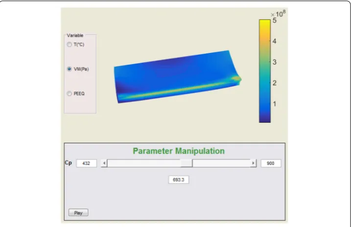
A demonstrator has been programmed for the visualization of the resulting space–time (4D)computational vademecum(see Fig.12). One recalls that there is no FE computation at the online phase. Interpolating a new space–time solution with the proposed adapta-tion approach is done in real time. CPU time for the thermo-mechanical fields of a new parameter is less than 0.1 s, whereas it takes about 7 h to perform a full FE computations with a single processor (see Table4). Although the offline CPU time for constructing the snapshots may be expensive, it will reduce much more time in the use of thecomputational vademecumat the online phase for computing parametric solutions with optimization or identification purpose. Furthermore, the necessary memory to perform the online inter-polation is less than 500 Mb in this example. It means that thecomputational vademecum can be used either with a laptop or even a smartphone.
Fig. 12 Demonstrator of Space–timecomputational vademecumdeveloped in matlab
Table 4 CPU time for a new solution
Phase Proposed approach (6 snapshots, error<1%) Standard FEM
Offline ≈42 h –
Fig. 13 Space–time yield stresscomputational vademecum
4D⊗1D mechanicalcomputational vademecum
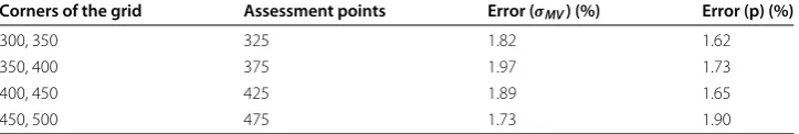
A similarcomputational vademecumis made for a mechanical parameter: the material initial yield stressσy(MPa)∈D=[300, 500]. The minimal set of snapshots that should be taken into account for building thecomputational vademecum(see Fig.13) with an error smaller than 2% is obtained by the sampling points{300, 350, 400, 450, 500}(see Table5). The online space–time response is given in real time with a high computation time reduction (Table6). Optimal memory storage is obtained by space–time separated variable representation of the RBs.
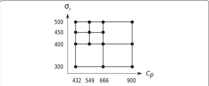
4D⊗2Dcomputational vademecum
LetD=DC ×Dσ be a 2D parameter space withCp(J·kg−1·K−1)∈ DC =[432, 900] andσy(MPa)∈ Dσ = [300, 500]. This time, parametric studies are considered in the square 2D-domainD. The snapshots selected by the proposed approach are shown in Fig.14for an guaranteed error smaller than 7% (see Table7). A 4D⊗2Dcomputational
Table 5 RB errors of von Mises stress and plastic strain
Corners of the grid Assessment points Error (σMV) (%) Error (p) (%)
300, 350 325 1.82 1.62
350, 400 375 1.97 1.73
400, 450 425 1.89 1.65
450, 500 475 1.73 1.90
Table 6 CPU time and memory (yield stresscomputational vademecum)
Phase CPU time (5 snapshots, error<2%) Memory
Full calculations ≈35 h 10 Gb
RB storage – 100 Mb
Fig. 14 Snapshots (black circles) selected in the 2D parameter space
Table 7 RB errors of von Mises stress and plastic strain in the 2D parameter space
Assessment points Error (σVM) (%) Error (p) (%)
(549, 350) 4.51 5.68
(783, 350) 4.45 5.09
(783, 450) 5.62 6.49
(490.5, 425) 2.57 1.92
(607.5, 425) 2.52 2.02
(607.5, 475) 2.65 2.24
(490.5, 475) 2.67 2.71
Fig. 15 Space–time 2Dcomputational vademecum
Table 8 CPU time and memory (4D⊗2Dcomputational vademecum)
Phase CPU time (14 snapshots, error<7%) Memory
Full calculations ≈98 h 10 Gb
RB storage – 220 Mb
Online <0.5 s <500 Mb
Fig. 16 Front sight of 3D welding with variable loading power
Computational vademecumfor real-time process control of welding
Let us consider a welding problem with a moving thermal load at a constant velocity over the work-piece with a possible change of input power at mi-time t2f (see Fig.16). In order to control the quality of welded piece and make real-time decisions to adaptQ1andQ2,
real-time simulations are required.
Assuming thatQi|i=1,2∈[8 12]×106W·m−2, the real-timecomputational vademecum
is then constructed using the proposed approach in the 2D parameter space for an error
less than 5%. Real time solutions are obtained for any value of input power in the parameter space. As depicted in Fig.17, one can modify the input power according to the real-time evolution of stress, here is an example obtained forQ1=8.5, Q2=11.5×10⁶W·m−2.
The online use ofcomputational vademecumcan help engineers make real time decisions for the input power of welding to control the quality of work-pieces.
Conclusion
Quasi-optimal space–time computational vademecumdedicated to parametric studies of welding process is constructed with a non-intrusive strategy. The reducibility of the full transient thermo-elasto-plastic model is studied by SVD analysis. It is shown that the reducibility of the transient thermal problem is significantly improved when the RBs are pre-computed in the moving frame. The proposed approach is based on a space– time Grassmann manifold interpolation of the reduced bases. This ensures high level of efficiency and accuracy for real time simulations and significantly reduces the high cost of computations for parametric studies. Furthermore, a localized multigrid selection method is presented. It leads to an appropriate selection of the sampling points in the parameter space that guarantee the accuracy of the space–timecomputational vademecum. Thus, the exhaustive generation of snapshots in the parameter space is avoided.
The proposed approach is applied to a 3D transient non-linear thermo-mechanical welding model with a moving heat Source. space–timecomputational vademecumsare obtained for a given quantity of interest (residual stress), for both thermal and mechanical parametric studies. Excellent results have been obtained for the RBs accuracy, memory storage and the online phase computations (real time). Indeed, online phase CPU time is less than 0.5s and limited memory storage is required with a guaranteed acceptable error. As one of applications of thecomputational vademecum(parametric solutions), fast identification of problem parameters can be straightforwardly expected. In addition, real time process control can be expected as well by considering loading-related parameters.
Extension to multiparametric (high-dimensional) analysis is in progress with application to industrial software. In this case, the main challenge will be the development of a strategy sampling efficiently the parameter space for high-dimensional problems.
Authors’ contributions
All authors have prepared the manuscript. All authors read and approved the final manuscript.
Acknowledgements
The authors gratefully acknowledge AREVA and SAFRAN for funding of this work within the framework of the “Life extension and manufacturing processes” teaching and research Chair.
Competing interests
The authors declare that they have no competing interests.
Availability of data and materials
Not applicable.
Consent for publication
Not applicable.
Ethics approval and consent to participate
Not applicable.
Funding
Publisher’s Note
Springer Nature remains neutral with regard to jurisdictional claims in published maps and institutional affiliations.
Received: 8 March 2017 Accepted: 6 January 2018
References
1. Chinesta F, Leygue A, Bordeu F, Aguado J, Cueto E, González D, Alfaro I, Ammar A, Huerta A. Pgd-based computational vademecum for efficient design, optimization and control. Arch Comput Methods Eng. 2013;20(1):31–59.
2. Courard A, Néron D, Ladeveze P, Andolfatto P, Bergerot A. Virtual charts for shape optimization of structures. In: 2nd ECCOMAS Young investigators conference (YIC 2013). 2013.
3. Vitse M, Néron D, Boucard PA. Virtual charts of solutions for parametrized nonlinear equations. Comput Mech. 2014;54(6):1529–39.
4. Niroomandi S, Alfaro I, Cueto E, Chinesta F. Model order reduction for hyperelastic materials. Int J Numer Methods Eng. 2010;81(9):1180–206.
5. Hotelling H. Analysis of a complex of statistical variables into principal components. J Educ Psychol. 1933;24(6):417. 6. Loeve M. Probability theory, the university series in higher mathematics. NJ: Princeton University Press; 1960. 7. Lorenz EN. Empirical orthogonal functions and statistical weather prediction. Cambridge, USA: Massachusetts
Institute of Technology; 1956.
8. Karhunen K. Über lineare Methoden in der Wahrscheinlichkeitsrechnung. Helsinki: Universitat Helsinki; 1947. 9. Loève M. Probability theory: foundations, random sequences. New York: D. Van Nostrand Company; 1955. 10. Fritzen F, Böhlke T. Three-dimensional finite element implementation of the nonuniform transformation field
analysis. Int J Numer Methods Eng. 2010;84(7):803–29.
11. Hernández J, Oliver J, Huespe AE, Caicedo M, Cante J. High-performance model reduction techniques in computational multiscale homogenization. Comput Methods Appl Mech Eng. 2014;276:149–89.
12. Holmes P, Lumley JL, Berkooz G. Turbulence, coherent structures, dynamical systems and symmetry. Cambridge: Cambridge university press; 1998.
13. Kerfriden P, Gosselet P, Adhikari S, Bordas SPA. Bridging proper orthogonal decomposition methods and augmented newton-krylov algorithms: an adaptive model order reduction for highly nonlinear mechanical problems. Comput Methods Appl Mech Eng. 2011;200(5):850–66.
14. Kunisch K, Volkwein S. Galerkin proper orthogonal decomposition methods for parabolic problems. Numerische mathematik. 2001;90(1):117–48.
15. Yvonnet J, He QC. The reduced model multiscale method (r3m) for the non-linear homogenization of hyperelastic media at finite strains. J Comput Phys. 2007;223(1):341–68.
16. Chinesta F, Ammar A, Cueto E. Recent advances and new challenges in the use of the proper generalized decomposition for solving multidimensional models. Arch Comput Methods Eng. 2010;17(4):327–50. 17. Chinesta F, Cueto E. PGD-based modeling of materials, structures and processes. Berlin: Springer; 2014. 18. Chinesta F, Ladeveze P, Cueto E. A short review on model order reduction based on proper generalized
decomposition. Arch Comput Methods Eng. 2011;18(4):395–404.
19. Ladeveze P, Passieux JC, Néron D. The latin multiscale computational method and the proper generalized decomposition. Comput Methods Appl Mech Eng. 2010;199(21):1287–96.
20. Ladevèze P. Sur une famille d’algorithmes en mécanique des structures. Comptes rendus des séances de l’Académie des sciences. Série 2, Mécanique-physique, chimie, sciences de l’univers, sciences de la terre. 1985;300(2):41–4. 21. Ladevèze P. Nonlinear computational structural mechanics: new approaches and non-incremental methods of
calculation. New York: Springer; 2012.
22. Boisse P, Bussy P, Ladeveze P. A new approach in non-linear mechanics: the large time increment method. Int J Numer Methods Eng. 1990;29(3):647–63.
23. Cognard JY, Ladevèze P. A large time increment approach for cyclic viscoplasticity. Int J Plast. 1993;9(2):141–57. 24. Relun N, Néron D, Boucard P. A model reduction technique based on the pgd for elastic-viscoplastic computational
analysis. Comput Mech. 2013;51(1):83–92.
25. Boucinha L, Gravouil A, Ammar A. Space–time proper generalized decompositions for the resolution of transient elastodynamic models. Comput Methods Appl Mech Eng. 2013;255:67–88.
26. Giacoma A, Dureisseix D, Gravouil A, Rochette M. A multiscale large time increment/fas algorithm with time-space model reduction for frictional contact problems. Int J Numer Methods Eng. 2014;97(3):207–30.
27. Ryckelynck D. A priori hyperreduction method: an adaptive approach. J Comput Phys. 2005;202(1):346–66. 28. Ammar A, Ryckelynck D, Chinesta F, Keunings R. On the reduction of kinetic theory models related to finitely
extensible dumbbells. J Non-Newtonian Fluid Mech. 2006;134(1):136–47.
29. Chinesta F, Ammar A, Falco A, Laso M. On the reduction of stochastic kinetic theory models of complex fluids. Model Simul Mater Sci Eng. 2007;15(6):639.
30. Chinesta F, Ammar A, Lemarchand F, Beauchene P, Boust F. Alleviating mesh constraints: model reduction, parallel time integration and high resolution homogenization. Comput Methods Appl Mech Eng. 2008;197(5):400–13. 31. Zhang Y, Combescure A, Gravouil A. Efficient hyper reduced-order model (HROM) for parametric studies of the 3D
thermo-elasto-plastic calculation. Finite Elem Anal Des. 2015;102:37–51.
32. Ammar A, Mokdad B, Chinesta F, Keunings R. A new family of solvers for some classes of multidimensional partial differential equations encountered in kinetic theory modeling of complex fluids. J Non-Newtonian Fluid Mech. 2006;139(3):153–76.
34. Pruliere E, Chinesta F, Ammar A. On the deterministic solution of multidimensional parametric models using the proper generalized decomposition. Math Comput Simul. 2010;81(4):791–810.
35. Ghnatios C, Masson F, Huerta A, Leygue A, Cueto E, Chinesta F. Proper generalized decomposition based dynamic data-driven control of thermal processes. Comput Methods Appl Mech Eng. 2012;213:29–41.
36. Ammar A, Huerta A, Chinesta F, Cueto E, Leygue A. Parametric solutions involving geometry: a step towards efficient shape optimization. Comput Methods Appl Mech Eng. 2014;268:178–93.
37. Niroomandi S, González D, Alfaro I, Bordeu F, Leygue A, Cueto E, Chinesta F. Real-time simulation of biological soft tissues: a pgd approach. Int J Numer Methods Biomed Eng. 2013;29(5):586–600.
38. Chaturantabut S, Sorensen DC. Nonlinear model reduction via discrete empirical interpolation. SIAM J Sci Comput. 2010;32(5):2737–64.
39. Niroomandi S, Alfaro I, Cueto E, Chinesta F. Real-time deformable models of non-linear tissues by model reduction techniques. Comput Methods Programs Biomed. 2008;91(3):223–31.
40. Niroomandi S, Alfaro I, Cueto E, Chinesta F. Accounting for large deformations in real-time simulations of soft tissues based on reduced-order models. Comput Methods Programs Biomed. 2012;105(1):1–12.
41. Amsallem D, Farhat C. Interpolation method for adapting reduced-order models and application to aeroelasticity. AIAA J. 2008;46(7):1803–13.
42. Maday Y, Patera AT, Turinici G. A priori convergence theory for reduced-basis approximations of single-parameter elliptic partial differential equations. J Sci Comput. 2002;17(1–4):437–46.
43. Maday Y, Rønquist EM. A reduced-basis element method. J Sci Comput. 2002;17(1–4):447–59.
44. Rozza G, Huynh DBP, Patera AT. Reduced basis approximation and a posteriori error estimation for affinely parametrized elliptic coercive partial differential equations. Arch Comput Methods Eng. 2008;15(3):229–75. 45. Veroy K, Patera AT. Certified real-time solution of the parametrized steady incompressible navier-stokes equations:
rigorous reduced-basis a posteriori error bounds. Int J Numer Methods Fluids. 2005;47(8–9):773–88.
46. Balagangadhar D, Dorai G, Tortorelli D, of Illinois at Urbana-Champaign U. A displacement-based reference frame formulation for steady-state thermo-elasto-plastic material processes. Int J Solids Struct. 1999;36(16):2397–416. 47. Rajadhyaksha SM, Michaleris P. Optimization of thermal processes using an eulerian formulation and application in
laser surface hardening. Int J Numer Methods Eng. 2000;47(11):1807–23.
48. Canales D, Leygue A, Chinesta F, González D, Cueto E, Feulvarch E, Bergheau JM, Huerta A. Vademecum-based gfem (v-gfem): optimal enrichment for transient problems. Int J Numer Methods Eng. 2016;108:971–89.
49. Bergheau J, Pont D, Leblond J. Three-dimensional simulation of a laser surface treatment through steady state computation in the heat source’s comoving frame. In: Mechanical effects of welding, Springer; 1992, p. 85–92. 50. Gu M, Goldak J, Knight A, Bibby M. Modelling the evolution of microstructure in the heat-affected zone of steady
state welds. Can Metall Q. 1993;32(4):351–61.
51. Eckart C, Young G. The approximation of one matrix by another of lower rank. Psychometrika. 1936;1(3):211–8. 52. Absil PA, Mahony R, Sepulchre R. Riemannian geometry of grassmann manifolds with a view on algorithmic
computation. Acta Applicandae Mathematica. 2004;80(2):199–220.
53. Edelman A, Arias TA, Smith ST. The geometry of algorithms with orthogonality constraints. SIAM J Matrix Anal Appl. 1998;20(2):303–53.
54. Boothby WM. An introduction to differentiable manifolds and Riemannian geometry. Houston: Gulf Professional Publishing; 2003.
55. Amsallem D. Interpolation on manifolds of cfd-based fluid and finite element-based structural reduced-order models for on-line aeroelastic predictions. Ph.D. thesis, Stanford University. 2010.
56. Absil PA, Mahony R, Sepulchre R. Optimization algorithms on matrix manifolds. New Jersey: Princeton University Press; 2009.
57. Begelfor E, Werman M. Affine invariance revisited. In: null, IEEE; 2006. p. 2087–94.
58. De Boor C, Ron A. Computational aspects of polynomial interpolation in several variables. Math Comput. 1992;58(198):705–27.