Robust sound event classification with bilinear multi-column ELM-AE and two-stage ensemble learning

R E S E A R C H

Open Access

Robust sound event classification with

bilinear multi-column ELM-AE and

two-stage ensemble learning

Junjie Zhang

, Jie Yin

, Qi Zhang

, Jun Shi

and Yan Li

Abstract

The automatic sound event classification (SEC) has attracted a growing attention in recent years. Feature extraction is a critical factor in SEC system, and the deep neural network (DNN) algorithms have achieved the state-of-the-art performance for SEC. The extreme learning machine-based auto-encoder (ELM-AE) is a new deep learning algorithm, which has both an excellent representation performance and very fast training procedure. However, ELM-AE suffers from the problem of unstability. In this work, a bilinear multi-column ELM-AE (B-MC-ELM-AE) algorithm is proposed to improve the robustness, stability, and feature representation of the original ELM-AE, which is then applied to learn feature representation of sound signals. Moreover, a B-MC-ELM-AE and two-stage ensemble learning (TsEL)-based feature learning and classification framework is then developed to perform the robust and effective SEC. The experimental results on the Real World Computing Partnership Sound Scene Database show that the proposed SEC framework outperforms the state-of-the-art DNN algorithm.

Keywords:Sound event classification, Multi-column, Bilinear, Extreme learning machine auto-encoder, Ensemble learning

1 Introduction

Sound event classification (SEC), also known as acoustic event classification (AEC), which aims to assign a se-mantic label to the audio content of a short sound chip [1, 2], is attracting a growing attention in recent years. SEC has wide potential applications [3], such as acoustic surveillance, bioacoustic monitoring, and environmental sound supervising [1–3].

The SEC system usually consists of three components, namely, signal preprocessing, feature extraction, and classification [2]. As a critical factor for the performance of SEC, feature extraction is a challenging task in SEC, and many efforts have been devoted to extract effective feature representation. The commonly extracted features for SEC can be roughly divided into the following cat-egories [2]: temporal domain features, frequency domain features, time-frequency image features, cepstral features,

modulation frequency features, eigen domain features, and phase space features. However, most of these features are hand-crafted descriptors, which are at a low semantic level, and also generic for different sound datasets without data specificity [4].

In contrast to the hand-crafted features, the learning-based feature representation methods have gained their good reputation for SEC in recent years because they are data-specific and robust, and the learned features have a higher semantic level [4]. The typical feature learning methods for SEC include bag of words [5], sparse coding [6], exemplar-based coding [7], and deep learning (DL) [8]. Specially, DL has achieved great success in image and speech signal processing by developing a layered, hierarchical architecture to yield high-level and more effective data representation [9–11]. DL has also been applied to SEC and performs superiorly to the com-monly used hand-crafted features [8, 12, 13]. McLough-lin et al. proposed to use deep neural network (DNN) classifier for representing the time-frequency features from the stabilized auditory image (SAI) and spectro-gram image features (SIF), respectively, for SEC [8]. Notably, this DNN algorithm can effectively improve * Correspondence:[email protected];[email protected]

2_{School of Communication and Information Engineering, Shanghai}

University, Shanghai, China

3_{College of Computer Science and Software Engineering, Shenzhen}

University, Shenzhen, China

Full list of author information is available at the end of the article

feature representation of original time-frequency fea-tures and then promote the classification performance [8]. Other DL algorithms, such as deep belief network (DBN) [13], convolutional neural networks (CNN) [14, 15], and auto-encoder (AE) [16], have also been effect-ively used for SEC. However, it is still time-costing to train a deep network model by these DL algorithms for a large-scale sound dataset.

The extreme learning machine (ELM) is a supervised learning algorithm based on single-layer feedforward neural networks (SLFNs), which randomly assigns the weights to the input layer and analytically fixes the weights between the hidden layer and the output layer [17]. ELM offers significant advantages, such as fast learning speed, effective performance, and ease of

imple-mentation [17–19]. Therefore, ELM has become a

popu-lar tool for solving various classification and regression tasks.

Although AE is an effective unsupervised DL algo-rithm for SEC, it also suffers from the problem of time-costing training. Recently, Kasun et al. proposed a novel extreme learning machine-based auto-encoder (ELM-AE) algorithm for unsupervised feature learning from large-scale data [20]. ELM-AE is a special case of ELM in essence, in which the input is equal to the output, and the randomly generated weights are chosen to be orthogonal together with the bias of hidden layers [20]. ELM-AE is no longer an iterative algorithm, and it adopts a similar solution procedure to ELM to improve the training speed. Therefore, ELM-AE has not only an excellent representation performance with multi-layer ELM-AE networks but also an extremely fast training stage, which is several orders of magnitude faster than other DL algorithms [20].

ELM-AE has attracted considerable attentions in re-cent years, and its variants have also been proposed for different applications [21–25]. However, all these ELM-AE-based algorithms generally suffer from the problem that the random input-layer weights in ELM-AE net-works usually result in unstable performance. To im-prove its stability, we propose a bilinear multi-column ELM-AE (B-MC-ELM-AE) algorithm to robustly learn feature representation and then apply it to SEC.

The multi-column deep neural network (MC-DNN) is a newly proposed DL method inspired by the microcol-umns of neurons in the cerebral cortex. MC-DNN trains several deep neural columns as experts to unfold their potentials and improve representation performance [26]. Ciresan et al. combined multiple DNN columns by averaging their outputs that were trained on inputs with different standard preprocessing methods, and this MC-DNN algorithm outperformed the compared DL algorithms on several public image datasets [26]. Agostinelli et al. developed a multi-column-based

stacked sparse AE algorithm for image denoising by calculating the optimal column weights via solving a nonlinear optimization program [27]. Shao et al. pro-posed a multispectral neural networks algorithm to learn robust feature representation from MC-DNN, which achieved superior performance for image classi-fication [28]. All these studies indicate the effective-ness of multi-column method in DL.

ELM-AE has the potential to be extended to a multi-column version, from which the learned multi-channel features can be further fed to an ensemble learning al-gorithm for classification. Moreover, ELM-AE is also suitable for implementing the multi-column operation, since each column of ELM-AE has a very fast training speed. Therefore, this multi-column-based ELM-AE (MC-ELM-AE) algorithm will consequentially improve the robustness, stability, and classification performance. On the other hand, the bilinear model has been successfully applied to CNN, which multiplies the convolutional-layer outputs of two-channel CNNs at each location of the image, resulting in bilinear features [29]. This bilinear outer product can capture pairwise correlations between the feature channels to help im-prove feature representation. While from the perspective of kernel functions, bilinear features are closely similar to the quadratic kernel, which gives a linear classifier the discriminative power of a quadratic kernel machine [30]. Therefore, the bilinear model can be effectively used for feature representation [29, 30], which is also feasible for AE to build a bilinear model-based MC-ELM-AE (B-MC-ELM-MC-ELM-AE); that is to say, the bilinear model can be applied to each pair of ELM-AE columns to fur-ther improve the robust feature representation.

In this study, we propose a feature learning and clas-sification framework for SEC with B-MC-ELM-AE and two-stage ensemble learning (TsEL), in which a B-MC-ELM-AE algorithm learns the robust feature represen-tation of sound segments, and then, a two-stage ensemble learning algorithm is used to fuse features from B-MC-ELM-AE and classify sound events. The main contributions are threefold: (1) A MC-ELM-AE algorithm is proposed to achieve the robust feature repre-sentation for sound signals; (2) A B-MC-ELM-AE algo-rithm is proposed to capture pairwise correlations among multiple ELM-AE columns for further improving feature representation and robustness; (3) A TsEL framework is proposed as a classifier to fuse the decisions of B-MC-ELM-AE to promote classification performance.

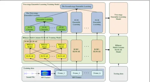
2 B-MC-ELM-AE- and TsEL-based robust SEC framework

operation is performed on a sound file to generate fea-tures for each segmented frame, which has the same length for analysis [8]. The B-MC-ELM-AE algorithm is then implemented on the SIF features for each frame to learn more effective feature representation, which will generate multiple-channel bilinear features. Next, in the first stage of the TsEL component, single-channel bilin-ear features are first fed to an ELM classifier to generate classification decision values, which are then fused by the weighted-voting-based ensemble learning algorithm to achieve the decision of the current frame. Finally, the second-stage ensemble learning algorithm is conducted on all the frames belonging to a sound file to fuse their decisions and yield the final classification result for SEC. It is worth noting that in the conventional SEC frame-work, only one stage of ensemble learning is used to in-tegrate the classification results of different frames in one sound file. However, an additional ensemble learn-ing is adopted to fuse multiple B-MC-ELM-AE in our proposed framework.

2.1 SIF feature extraction

As introduced in [8], in order to extract the SIF features, the fast Fourier transform (FFT) is performed and a stack of FFT magnitude spectra builds the initial spectrogram. For the current frameF, spectral linefFis given by

f_Fð Þ ¼k X_nw_¼s−₀1

sFð Þne −j2πnk

ws

fork¼1⋯ ws 2 −1

ð

1Þ

With

sFð Þ ¼n s Fð ⋅σþnÞ⋅w nð Þ for n¼0⋯ðws−1Þ ð2Þ

where σ is the sample advance between analysis frames

and w(n) defines an N-point Hamming window. Then,

down sampling is then implemented by averaging over

B'

= [ws/2B] samples, where Bis the number of bin

fre-quency resolution. The resulting spectrum are stacked to form an overlap spectrogram as

S lð; mÞ ¼_B1₀XB_n¼0⋅ð_Bl0þ_⋅l1ÞfF−mð Þn

for l¼0⋯B=σ

ð3Þ

The spectrogramS includes a history of up toD

con-secutive spectral lines, which are concatenated to form a (B⋅D+ 1) dimension feature vector, called spectrogram image feature (SIF). This feature vector is augmented by a scalar energy metric, which is defined by

v¼X

D−1

l¼0

XB−1

m¼0

S lð;mÞ ð4Þ

Please refer to [8] for details about SIF feature extraction.

2.2 ELM-AE algorithm

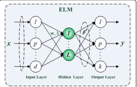
ELM is an effective SLFN-based learning algorithm with randomly generated hidden nodes as shown in Fig. 2 [17–19]. The ELM theory can also be applied to build a multi-layer AE, which performs layer-by-layer unsuper-vised learning [20, 22].

For a training set {(xi,yi),i= 1,…,n}, where xi is the

training sample and yi is the label, the input data x is

mapped to the ELM random feature space with the net-work output by

f_Lð Þ ¼x XL_i¼1βihið Þ ¼x h xð Þβ ð5Þ

where L is the number of nodes in hidden layer,βi

de-notes the weight connecting theith hidden node and the output layer, and hi(x) is the hidden node output

(non-linear feature mapping) for inputxby

hið Þ ¼x g wð i⋅xþbiÞ ð6Þ

wherewiis the weight vector connecting the ith hidden

node and the input nodes, bi is the bias of ith hidden

node, andg(x) is the activation function.

The ELM then aims to solve the following problem:

Y¼Hβ ð7Þ

Where Y= [y1,…yn]T and H= [hT(x1),…, hT(xn)]T. The

output weightsβcan be calculated by

β¼H†_Y¼HT_HHT−1 _ð8Þ

where H† is the Moore-Penrose generalized inverse of

matrix H. By adding a regularization term to improve

the generalization performance and make the solution more robust, the resulting solutionβis given by [18, 19]

β¼ HT_Hþ I

C

−1

HT_{Y ð9Þ}

where C is a parameter to balance the experiential risk

and structural risk.

On the other hand, AE is a popular unsupervised fea-ture learning model, which aims to make the encoded outputs to be equal to the original inputs by minimizing the reconstruction errors [31]. As a variant of AE, ELM-based AE (ELM-AE) significantly improves the training speed [20] and also achieves excellent representation performance by building multi-layer networks [22].

Figure 3 shows the network architectures of ELM-AE. In ELM-AE, the input data is first transformed into an ELM random feature space, and then, a multi-layer un-supervised learning is conducted to achieve high-level feature representation.

For a single-layer ELM-AE, the input data is projected to a new space with the constraint of the orthogonal random weights and biases of the hidden nodes on Eq. (10) by

H¼gðw⋅xþbÞ s:t: wTw¼Iand bTb¼1 ð10Þ

The output weight β is now responsible for learning

transformation from the feature space to input data, and it can be determined analytically as ELM with the simi-lar form:

β¼ HT_Hþ I

C

−1

HT_{X ð11Þ}

whereXis the input data.

The multi-layer ELM-AE can then be implemented to learn higher level feature representation based on single-layer ELM-AE network architectures. Here, we rewrite the equation of the output of each hidden layer as

Hi¼gðHi−1⋅βÞ ð12Þ

where Hi and Hi−1 are the outputs of the ith and the

(i-1)th layers, respectively. Notably, each hidden layer of ELM-AE works as an independent and separated fea-ture extractor.

2.3 Bilinear multi-column ELM-AE

In order to suppress the effect of unstability deriving from random weights and improve the robustness to-gether with representation performance, we proposed the B-MC-ELM-AE algorithm.

As shown in Fig. 1, several column ELM-AEs are per-formed on the same input data and fused to form the multi-column ELM-AE (MC-ELM-AE) algorithm. Since multi-column features are generated from MC-ELM-AE, the feature concatenation is the simplest way to fuse these features.

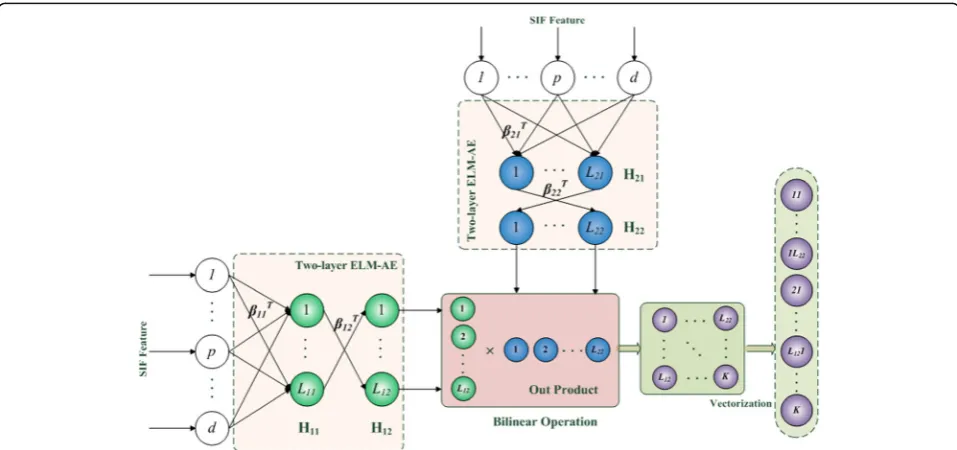
In this work, we use the bilinear model to pairwisely fuse the features of MC-ELM-AE to improve representa-tion and further boost classificarepresenta-tion performance as shown in Fig. 4, which is similar to the bilinear CNN model [29]. The bilinear features are the outer product

of a pair of ELM-AE features. Define E1 and E2 as the

learned features of two ELM-AEs from the same input data; the bilinear feature representation is calculated by

EB¼E1⊗E2¼E1⋅ET2 ¼

e1 1

e2 1

⋮

em

1

2 6 6 4

3 7 7

5 e12 e22⋯e

n

2

¼

z11 _{⋯ z}1n

⋮ ⋱ ⋮

zm1 _{⋯ z}mn

2 6 4

3 7

5 ð13Þ

where m and n are the feature dimensionalities of E1

andE2, respectively.

The calculated bilinear representation EB is a matrix, which is then vectorized to a vector formebas the input

of a classifier in this work. Since there is no back propa-gation in ELM-AE, the bilinear feature representation is

very straightforwardly embedded in ELM-AE. For the k

column MC-ELM-AEs,k× (k−1)/2 channel bilinear

fea-tures in total are obtained by the pairwise bilinear oper-ation, which are then fed to the TsEL framework for classification.

2.4 Two-stage ensemble learning framework

The multi-channel bilinear features from one sound frame are more robust and effective than the original single-column ELM features, which can be used for clas-sification of the current frame. Since a sound file is di-vided into multiple frames, the final classification result of a sound file is the fused decision of all frames. In this work, a two-stage ensemble learning (TsEL) framework is proposed for SEC with B-MC-ELM-AE features, since Fig. 3The network architecture of ELM-AE

ensemble learning can improve the generalization and prediction performance of multiple classifiers by com-bining their decisions.

Specifically, as shown in Fig. 1, the first-stage ensemble learning is implemented on the base ELM classifiers of the multi-channel bilinear features generated from B-MC-ELM-AE for each sound frame, and the second-stage ensemble learning is conducted on all the decisions of all frames to provide final SEC. It is worth noting that various ensemble learning algorithms can be used in this TsEL framework.

A weighted-voting-based ensemble learning algorithm is used in the first-stage learning [32], which is very sim-ple and effective.

Define the classification decisions of all ELM classifiers on individual bilinear features of B-MC-ELM-AE as

Ŷ= [Ŷ1(x),Ŷ2(x),⋯,Ŷk(x) ]T, where k is the number

of all base ELM classifiers, andŶi(x) means the output of ith base classifier on sample x. Suppose that the total weight matrix of all of base classifiers is given by W0_{¼ w}0

1; w 0 2;⋯;w

0

k

T

, wherew0ijði¼1;⋯;k; j¼1;2;⋯;mÞ means the weight of the ith base classifier on the jth class. The weight of each base classifier is calculated as

w0

ij¼

logðpij=ð1−pijÞÞ Xt

i¼1logðpij=ð1−pijÞÞ

; i¼1;2;⋯k; j¼1;2;⋯m

-(14) wherepijis the classification accuracy of theith classifier

on thejth class. The final decision of this multi-classifier ensemble learning is given by the maximum score based on Eqs. (15) and (16)

sj¼

X

i¼1

k _w0

ij⋅Y^ij; j¼1;2;⋯;m ð15Þ

wheresjis the score of the jth class. The final

classifica-tion result is decided by

Label¼argmax sð1; s2;s3;⋯;smÞ ð16Þ

Since different sound files have different sound lengths, resulting in different frame numbers, some sim-ple ensemble learning algorithms, such as majority vot-ing and weighted votvot-ing [8], can be used in the second-stage ensemble learning in our framework to fuse the decisions of all multiple sound frames from the first stage to generate the final classification decision for the current sound event.

3 Experiments and results 3.1 Dataset and data preprocessing

The performance of the proposed B-MC-ELM-AE-TsEL framework for SEC was evaluated on the Real World Computing Partnership (RWCP) Sound Scene Database in Real Acoustic Environments [33]. The noise-corrupted data use four background noise environments selected

from the NOISEX-92 database, namely “Destroyer

Con-trol Room,” “Speech Babble,” “Factory Floor1,” and “Jet Cockpit 1”[3]. In McLoughlin’s work, there were in total 50 classes of sound events selected from the RWCP Sound Scene Database, such as the wooden, metal and china im-pacts, friction sounds, bells, phones ringing, and whistles, and each class included 80 files.

McLoughlin et al. have achieved the state-of-the-art performance on this RWCP dataset with the DNN algo-rithm [8]. Thus, we directly used this dataset with ex-tracted SIF features in this study. Each sound file was segmented into several frames, and the SIF features were then extracted from each frame with a dimensionality of 721. The details about SIF features and data processing can be found in [8] and [3]. The proposed B-MC-ELM-AE algorithm was then implemented to learn feature representation from the extracted SIF features, and the learned features were further fed to the TsEL framework for SEC.

3.2 Experimental settings

We conducted two same experiments as those in [8] to evaluate our proposed SEC framework. In the first mis-matched condition experiment, the data in training set were exclusively clean sounds without noise, but the data in testing set were corrupted by additive back-ground noise at levels of 20, 10, and 0 dB SNR. The sec-ond experiment was the multi-csec-ondition evaluation, in which both the data in training set and testing set com-prised a variety of clean and noise-corrupted sounds. The 10-fold cross-validation strategy is performed for all algorithms, and the result of classification accuracy is given by the form of mean ± SD (standard deviation).

All the compared algorithms are listed as follows:

(i) DNN in [8]: the results of DNN by McLoughlin et al. in [8] were selected as the baseline.

(ii) SIF-ELM: the original SIF features of each sound segment were directly fed to the ELM classifier for classification, and then, only the second-stage ensemble learning was implemented to generate the final decision on all segments.

(iii) ELM-AE: the single-column ELM-AE was imple-mented on SIF features for each sound segment with the ELM classifier, and then, only the second-stage ensemble learning was used to get the final decision on all segments.

all segments. Notably, B-ELM-AE is a special case of B-MC-ELM-AE with two-column ELM-AEs. (v) MC-ELM-AE-C: the 5-column MC-ELM-AE was

conducted on SIF features for each sound segment to generate 5-column features, which were then concatenated to form a feature vector for the ELM classifier, and only the second-stage ensemble learning was used to get the final decision on all segments.

(vi) AE-TsEL-V: the 5-column MC-ELM-AE was conducted on SIF features for each sound segment to generate 5-column features, which were then fed to a TsEL algorithm. However, the

majority-voting-based ensemble learning algorithm was performed to boost the classification results of the 5-column features in the first-stage ensemble learning.

(vii) AE-TsEL-W: the 5-column MC-ELM-AE was conducted on SIF features for each sound segment to generate 5-column features, which were then fed to a TsEL algorithm with the weighted-voting-based ensemble learning algorithm in Section2.4.

(viii) B-MC-ELM-AE-C: the B-MC-ELM-AE was conducted on SIF features for each sound segment to generate 5-channel bilinear features, which were then concatenated to form a feature vector for the ELM classifier, and only the second-stage ensemble learning was used to get the final decision on all segments.

(ix) ELM-AE-TsEL-V: the proposed B-MC-ELM-AE and TsEL-based algorithm was conducted on SIF features for classification as shown in Fig.1. Here, the 5-column MC-ELM-AE was used for the bilinear model. However, the majority-voting-based ensemble learning algorithm was performed to boost the classification results of the pairwise bilinear features in the first-stage ensemble learning. (x)ELM-AE-TsEL-W: the proposed

B-MC-ELM-AE- and TsEL-based algorithm was conducted on SIF features for classification as shown in Fig.1

with the weighted-voting-based ensemble learning algorithm in Section2.4. Here, the 5-column MC-ELM-AE was used for the bilinear model.

It is worth noting that the following three ensemble learning methods were used in the second-stage of TsEL [8]: (1) the baseline method that considers the maximum class score from the mean of all predictive probability values of classifiers as the final decision (denoted as -b); (2) majority-voting-based ensemble learning (denoted as -v); (3) weighted-voting-based ensemble learning that weights the votes of individual classifiers by calculating the context energy (denoted as -e).

3.3 Results of the mismatched condition experiment

Tables 1, 2, and 3 show the classification results of dif-ferent algorithms for the first mismatched condition experiment with the -b, -v, and -e ensemble learning methods in the second stage of TsEL, respectively.

It can be found in Table 1 that all the ELM-AE-based algorithms outperform the baseline DNN algorithm in [8], showing the effectiveness of ELM-AE for SEC. The proposed B-MC-ELM-AE-TsEL-W algorithm achieves the best performance on all the clean condition, 20 , 10, and 0 dB SNR conditions, whose corresponding mean classification accuracies are 99.45 ± 0.30%, 97.00 ± 0.46%, 96.15 ± 1.26%, and 91.63 ± 1.29%, respectively. Compared with DNN, the B-MC-ELM-AE-TsEL-W algorithm im-proves accuracies by 2.72, 2.40, 5.88, and 15.16% at the clean, 20, 10, and 0 dB SNR conditions, respectively. Moreover, both MC-ELM-AE-TsEL-W and B-ELM-AE-TsEL-W outperform the majority-voting-based

MC-ELM-AE-TsEL-V and B-MC-ELM-AE-TsEL-V, which

indicates that the weighted-voting is more effective to boost multiple classifiers in this work. On the other hand, both B-ELM-AE and MC-ELM-AE algorithms are super-ior to the original ELM-AE, which indicates that the bilinear model and multi-column extension truly effect-ively improve the representation performance. Further-more, B-MC-ELM-AE achieves better performance than B-ELM-AE and MC-ELM-AE by fairly comparing the classification accuracy with the -C and -TsEL methods, respectively.

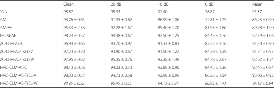
In Table 2, B-MC-ELM-AE-TsEL-W again obtains the best performance, whose mean accuracies are 98.95 ± 0.52%, 96.45 ± 0.55%, 94.15 ± 1.27%, and 86.93 ± 1.43% on the clean, 20, 10, and 0 dB SNR condition, respect-ively. Compared with DNN, B-MC-ELM-AE-TsEL-W achieves 1.12, 1.75, and 8.06% improvements for the 20, 10, and 0 dB SNR conditions, respectively. It also im-proves by at least 1.06% on the mean classification accuracy compared with all other algorithms. Again, the weighted-voting ensemble learning is superior the majority-voting case. However, with the -b ensemble learning method, the baseline DNN algorithm is slightly superior to other ELM-AE-based algorithms except B-MC-ELM-AE-TsEL-W on the clean, 20 and 10 dB SNR condition, while it dramatically degenerates on the 0 dB condition.

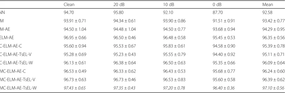
3.4 Results of the multi-condition evaluation experiment

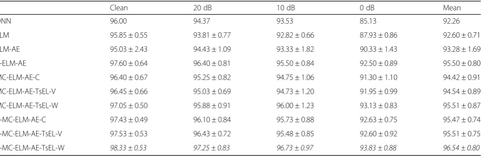
Tables 4, 5, and 6 give the results of different algorithms on the second multi-condition evaluation experiment with the -b, -v, and -e ensemble learning methods in the second stage of TsEL, respectively.

As can be seen from Table 4, B-MC-ELM-AE-TsEL-W outperforms all other algorithms, with mean classifica-tion accuracies of 98.65 ± 0.39%, 98.23 ± 0.45%, 98.18 ± 0.19%, and 96.90 ± 0.59% on the clean, 20, 10, and 0 dB SNR conditions, respectively. Here, there are no results given for the DNN algorithm with the -b ensemble learning method in [8].

It can be found in Table 5 that B-MC-ELM-AE-TsEL-W again achieves the best performance with the mean accuracies of 98.03 ± 0.36%, 97.40 ± 0.31%, 96.28 ± 1.05%, and 91.53 ± 0.84% on all the clean, 20, 10, and 0 dB SNR conditions, respectively, which improves by 1.13, 0.5, 3.08, and 11.13% compared with the baseline DNN algorithm.

In Table 6, almost all ELM-AE-based algorithms are superior to DNN, and B-MC-ELM-AE-TsEL-W is the best one. The mean accuracies of

B-MC-ELM-AE-TsEL-W are 97.43 ± 0.65%, 97.35 ± 0.43%, 97.20 ± 0.78% and 96.40 ± 0.36% on the clean, 20 dB, 10 dB and 0 dB SNR conditions, respectively, which improves by 2.73, 1.55, 5.10, and 8.70% compared with DNN.

4 Discussion

In this work, a feature learning and classification frame-work named B-MC-ELM-AE-TsEL is proposed for SEC. Generally, the learned features by ELM-AE are unstable due to the random input-layer weights in ELM-AE net-works, resulting in unstable performance. In order to improve the stableness of ELM-AE, the multi-column extension is proposed for ELM-AE to build MC-ELM-AE, whose multiple decisions are then fused by ensem-ble learning methods to generate more staensem-ble and robust performance. Moreover, the bilinear model is then ap-plied to MC-ELM-AE to mining the correlation among multiple ELM-AEs, and the TsEL strategy is proposed to improve the final decision. In the experiment, three levels of noise were added to clean sound data, namely, 20, 10, and 0 dB SNR conditions. With the increase of noise, the recognition performance for sound events

Table 1Classification results of different algorithms with the mean probability value ensemble learning (-b) at the second-stage TsEL (unit: %)

Clean 20 dB 10 dB 0 dB Mean

DNN 96.73 94.60 90.27 76.47 89.52

ELM 97.08 ± 0.45 90.31 ± 0.92 85.75 ± 1.16 72.39 ± 1.18 86.38 ± 0.93

ELM-AE 97.68 ± 1.31 94.25 ± 1.53 92.28 ± 2.04 86.63 ± 1.43 92.71 ± 1.58

B-ELM-AE 99.08 ± 0.34 95.88 ± 0.49 94.93 ± 0.93 89.85 ± 0.85 94.93 ± 0.65

MC-ELM-AE-C 98.63 ± 0.46 95.88 ± 0.67 94.35 ± 0.86 87.90 ± 1.27 94.19 ± 0.82

MC-ELM-AE-TsEL-V 98.53 ± 0.52 95.63 ± 0.55 93.73 ± 0.91 88.33 ± 1.48 94.05 ± 0.86

MC-ELM-AE-TsEL-W 99.03 ± 0.34 96.55 ± 0.52 95.53 ± 0.92 89.08 ± 1.61 95.05 ± 0.85

B-MC-ELM-AE-C 99.08 ± 0.35 96.08 ± 0.69 94.65 ± 1.07 89.93 ± 1.19 94.94 ± 0.83

B-MC-ELM-AE-TsEL-V 99.15 ± 0.31 96.20 ± 0.42 95.10 ± 0.88 90.45 ± 0.93 95.23 ± 0.63

B-MC-ELM-AE-TsEL-W 99.45 ± 0.30 97.00 ± 0.46 96.15 ± 1.26 91.63 ± 1.29 96.06 ± 0.83

Table 2Classification results of different algorithms with the context voting ensemble learning (-v) at the second-stage TsEL (unit: %)

Clean 20 dB 10 dB 0 dB Mean

DNN 98.87 95.33 92.40 78.87 91.37

ELM 93.76 ± 0.61 91.35 ± 0.62 86.99 ± 1.06 72.81 ± 1.29 86.23 ± 0.90

ELM-AE 95.53 ± 2.35 92.28 ± 1.67 89.40 ± 1.70 81.93 ± 1.86 89.78 ± 1.90

B-ELM-AE 98.23 ± 0.57 94.38 ± 0.67 92.50 ± 1.25 84.43 ± 1.76 92.39 ± 1.06

MC-ELM-AE-C 96.93 ± 0.65 93.70 ± 0.97 91.33 ± 0.83 83.25 ± 1.16 91.30 ± 0.90

MC-ELM-AE-TsEL-V 97.23 ± 0.70 93.90 ± 0.67 91.50 ± 1.22 84.20 ± 1.29 91.71 ± 0.97

MC-ELM-AE-TsEL-W 97.95 ± 0.62 95.35 ± 0.76 92.38 ± 1.49 84.78 ± 2.07 92.62 ± 1.24

B-MC-ELM-AE-C 98.13 ± 0.36 94.33 ± 0.73 92.88 ± 0.90 84.45 ± 1.36 92.45 ± 0.84

B-MC-ELM-AE-TsEL-V 98.33 ± 0.57 94.73 ± 0.58 92.98 ± 0.99 86.23 ± 1.54 93.06 ± 0.92

decreases for all algorithms used in this study. However, in the 0 dB SNR condition, the baseline DNN algorithm degenerates most rapidly compared with all the ELM-AE-based algorithms as shown in Tables 1, 2, 3, 4, 5, and 6, while the proposed B-MC-ELM-AE-TsEL algorithms, including both ELM-AE-TsEL-V and B-MC-ELM-AE-TsEL-W, still achieve good performance with a more than 90% mean accuracy only except the result in Table 2. Therefore, our B-MC-ELM-AE-TsEL framework is effective and robust for SEC, especially in the noisy environment.

There are three findings from the experimental results on RWCP Sound Scene Database: (1) the random input-layer weights in ELM-AE networks usually result in unstable performance, and the numbers of the hidden nodes in ELM-AE also lead to different feature represen-tations. Therefore, we propose the multi-column ELM-AE algorithm, which performs multiple ELM-ELM-AEs with different numbers of the hidden nodes on the same sound frame to generate diverse classification results. The first-stage ensemble learning is then conducted on the classification decisions of these multi-column ELM-AE to improve robustness and classification performance compared with the original ELM-AE algorithm; (2) the

bilinear model is then applied to each feature-pair of ELM-AE columns, in which the bilinear outer product can capture pairwise correlations between the feature channels for superior feature representation. The pro-posed B-MC-ELM-AE algorithm by integrating both bilinear and multi-column models into ELM-AE can fur-ther promote the representation performance and robustness for sound data; (3) the proposed B-MC-ELM-AE-TsEL framework is superior to the state-of-the-art DNN algorithm in [8] for SEC.

In the current B-MC-ELM-AE-TsEL framework, the B-MC-ELM-AE features are integrated by a classifier-or decision-level fusion method, that is to say, ensemble learning can be applied to all the classification results of individual column of B-ELM-AE. Specifically, a weighted-voting-based ensemble learning algorithm is used in the first-stage learning [32], which has shown its effectiveness compared with the majority-voting-based ensemble learning as shown in Tables 1, 2, 3, 4, 5, and 6. It should be noted that other ensemble

learn-ing algorithms, such as the margin distribution

optimization method and the Adaboost-based method [34, 35], also can be applied in this framework. On the other hand, instead of the classifier- or decision-level

Table 3Classification results of different algorithms with e-scaled weight ensemble learning (-e) at the second-stage TsEL (unit: %)

Clean 20 dB 10 dB 0 dB Mean

DNN 96.00 94.37 93.53 85.13 92.26

ELM 95.85 ± 0.55 93.81 ± 0.77 92.82 ± 0.66 87.93 ± 0.86 92.60 ± 0.71

ELM-AE 95.03 ± 2.43 94.43 ± 1.09 93.33 ± 1.82 90.33 ± 1.43 93.28 ± 1.69

B-ELM-AE 97.60 ± 0.64 96.40 ± 0.81 95.50 ± 0.84 92.50 ± 0.89 95.50 ± 0.80

MC-ELM-AE-C 96.40 ± 0.67 95.25 ± 0.82 94.75 ± 1.06 91.30 ± 1.10 94.42 ± 0.91

MC-ELM-AE-TsEL-V 96.45 ± 0.66 95.03 ± 0.69 94.73 ± 1.20 91.95 ± 0.99 94.54 ± 0.89

MC-ELM-AE-TsEL-W 97.05 ± 0.50 95.88 ± 0.91 96.00 ± 1.23 93.13 ± 0.83 95.51 ± 0.87

B-MC-ELM-AE-C 97.43 ± 0.49 96.10 ± 0.84 95.73 ± 0.88 92.63 ± 0.75 95.47 ± 0.74

B-MC-ELM-AE-TsEL-V 97.53 ± 0.53 96.43 ± 0.72 95.48 ± 0.85 92.60 ± 0.92 95.51 ± 0.75

B-MC-ELM-AE-TsEL-W 98.33 ± 0.53 97.25 ± 0.83 96.73 ± 0.97 93.83 ± 0.88 96.54 ± 0.80

Table 4Multi-condition (MC) classification results of different algorithms with the mean probability value ensemble learning (-b) at the second-stage TsEL (unit: %)

Clean 20 dB 10 dB 0 dB Mean

ELM 95.20 ± 0.59 94.06 ± 0.38 93.29 ± 0.69 89.42 ± 0.93 92.99 ± 0.65

ELM-AE 96.65 ± 0.85 96.03 ± 0.85 95.88 ± 0.78 94.35 ± 0.83 95.73 ± 0.83

B-ELM-AE 98.15 ± 0.24 98.03 ± 0.41 97.48 ± 0.31 95.95 ± 0.35 97.40 ± 0.33

MC-ELM-AE-C 97.20 ± 0.49 96.80 ± 0.72 96.43 ± 0.40 95.10 ± 0.72 96.38 ± 0.58

MC-ELM-AE-TsEL-V 96.93 ± 0.50 96.50 ± 0.64 96.15 ± 0.44 95.10 ± 0.89 96.17 ± 0.62

MC-ELM-AE-TsEL-W 97.95 ± 0.53 97.43 ± 0.47 97.55 ± 0.52 96.05 ± 0.77 97.25 ± 0.57

B-MC-ELM-AE-C 98.08 ± 0.54 97.65 ± 0.45 97.40 ± 0.47 96.08 ± 0.50 97.30 ± 0.49

B-MC-ELM-AE-TsEL-V 98.20 ± 0.35 97.9 ± 0.40 97.55 ± 0.45 96.03 ± 0.59 97.42 ± 0.45

fusion, another way to properly integrate these B-MC-ELM-AE features is the feature-level fusion. For ex-ample, the multiple kernel learning (MKL) method can effectively combine multiple-channel features and then make a decision, since the multiple kernels in MKL can naturally correspond to features from different views [36]. This feature-level fusion method will be studied for our B-MC-ELM-AE-TsEL framework in the future.

The proposed B-MC-ELM-AE-based two-stage ensem-ble learning algorithm has very fast learning speed, which is several orders of magnitude faster than other DL algorithms, resulting in short training time. More-over, the multi-channel ELM-AEs can perform in a par-allel way, which will improve the time efficiency. Therefore, our proposed algorithm is more suitable for real-time implementation than DNN in [8], because of its fast computational efficiency and high classification accuracy. However, since the multiple channels of ELM-AE should be trained to improve robustness and stabil-ity, B-MC-ELM-AE-based algorithm requires more

memory than DNN, mainly because the bilinear model is an operation of high-dimensional matrix. Therefore, dimensionality reduction can be conducted on ELM-AE features before bilinear operation. In current work, we only use the SIF features as the input to the proposed al-gorithm for a fair comparison with DNN in [8]. In fu-ture, we will select more features to evaluate the effect of input features on B-MC-ELM-AE and even directly perform B-MC-ELM-AE on the raw data or the features of time and frequency domain [37].

5 Conclusions

In conclusion, we propose a bilinear multi-column ELM-AE and two-stage ensemble learning-based feature learning and classification framework for SEC. The experimental results on RWCP Sound Scene Database indicate the robustness and effectiveness of B-MC-ELM-AE-TsEL framework. It suggests that the proposed framework has the potential for SEC.

Table 5Multi-condition (MC) classification results of different algorithms with context voting ensemble learning (-v) at the second-stage TsEL (unit: %)

Clean 20 dB 10 dB 0 dB Mean

DNN 96.90 96.90 93.20 80.40 91.85

ELM 93.34 ± 0.60 91.55 ± 0.57 89.22 ± 0.91 79.78 ± 1.62 88.47 ± 0.93

ELM-AE 94.23 ± 0.76 93.38 ± 1.49 91.65 ± 0.76 86.88 ± 1.60 91.54 ± 1.15

B-ELM-AE 97.38 ± 0.47 96.58 ± 0.47 95.10 ± 0.62 90.05 ± 1.35 94.78 ± 0.73

MC-ELM-AE-C 95.48 ± 0.63 94.70 ± 0.38 93.18 ± 0.91 88.73 ± 1.02 93.02 ± 0.74

MC-ELM-AE-TsEL-V 95.35 ± 0.57 94.35 ± 0.48 93.28 ± 0.82 89.00 ± 1.30 92.99 ± 0.79

MC-ELM-AE-TsEL-W 96.63 ± 0.31 95.35 ± 1.01 93.63 ± 1.02 89.50 ± 1.42 93.78 ± 0.94

B-MC-ELM-AE-C 97.13 ± 0.49 96.43 ± 0.62 94.88 ± 1.00 89.68 ± 0.97 94.53 ± 0.77

B-MC-ELM-AE-TsEL-V 97.33 ± 0.50 96.55 ± 0.60 95.38 ± 0.76 90.55 ± 0.72 94.95 ± 0.65

B-MC-ELM-AE-TsEL-W 98.03 ± 0.36 97.40 ± 0.31 96.28 ± 1.05 91.53 ± 0.84 95.81 ± 0.64

Table 6Multi-condition (MC) classification results of different algorithms with e-scaled weight ensemble learning (-e) at the second-stage TsEL (unit: %)

Clean 20 dB 10 dB 0 dB Mean

DNN 94.70 95.80 92.10 87.70 92.58

ELM 93.91 ± 0.71 94.34 ± 0.61 93.90 ± 0.86 91.51 ± 0.91 93.42 ± 0.77

ELM-AE 94.50 ± 1.04 94.48 ± 1.04 94.50 ± 0.77 93.68 ± 0.94 94.29 ± 0.95

B-ELM-AE 96.95 ± 0.66 96.50 ± 0.46 96.48 ± 0.58 95.45 ± 0.53 96.35 ± 0.56

MC-ELM-AE-C 95.60 ± 0.94 95.53 ± 0.67 95.83 ± 0.61 94.58 ± 0.90 95.39 ± 0.78

MC-ELM-AE-TsEL-V 95.28 ± 0.69 95.23 ± 0.43 95.55 ± 0.79 94.40 ± 0.92 95.11 ± 0.71

MC-ELM-AE-TsEL-W 96.13 ± 0.61 96.38 ± 0.64 96.50 ± 0.63 95.35 ± 0.66 96.09 ± 0.64

B-MC-ELM-AE-C 96.53 ± 0.49 96.33 ± 0.62 96.43 ± 0.53 95.68 ± 0.77 96.24 ± 0.60

B-MC-ELM-AE-TsEL-V 96.73 ± 0.63 96.73 ± 0.46 96.53 ± 0.83 95.60 ± 0.58 96.39 ± 0.62

Acknowledgements

This work is supported by the National Natural Science Foundation of China (61471231, 61401267, 61471245, U1201256), the Natural Science Foundation of Shenzhen City (JCYJ20140418091413514, JSGG20150529160945187, CXZZ20150424113738307).

Authors’contributions

YL and JS conceived and proposed the algorithm of this paper. JZ wrote the grogram of algorithms, and he also wrote the paper. JY performed the experiments and QZ revised the paper. All authors read and approved the final manuscript.

Competing interests

The authors declare that they have no competing interests.

Publisher’s Note

Springer Nature remains neutral with regard to jurisdictional claims in published maps and institutional affiliations.

Author details

1_{Key Laboratory of Specialty Fiber Optics and Optical Access Networks,}

School of Communication and Information Engineering, Shanghai University, Shanghai, China.2_{School of Communication and Information Engineering,} Shanghai University, Shanghai, China.3College of Computer Science and Software Engineering, Shenzhen University, Shenzhen, China.

Received: 12 August 2016 Accepted: 8 May 2017

References

1. D Stowell, D Giannoulis, E Benetos, M Lagrange, MD Plumbley, Detection and classification of acoustic scenes and events. IEEE Transactions on Multimedia17(10), 1733–1746 (2015)

2. RV Sharan, TJ Moir, An overview of applications and advancements in automatic sound recognition. Neurocomputing200, 22–34 (2016) 3. J Dennis, H Tran, ES Chng, Image feature representation of the subband

power distribution for robust sound event classification. IEEE Trans. Audio Speech Lang. Process.21(2), 367_–377 (2013)

4. H Phan, L Hertel, M Maass, R Mazur, A Mertins, Learning representations for nonspeech audio events through their similarities to speech patterns. IEEE Trans. Audio Speech Lang. Process.24(4), 807–822 (2016)

5. A Plinge, R Grzeszick, GA Fink, A bag-of-features approach to acoustic event detection (The 39th International Conference on Acoustics, Speech and Signal Processing (ICASSP), 2014), pp. 3704-3708.

6. X Lu, Y Tsao, S Matsuda, C Hori, Sparse representation based on a bag of spectral exemplars for acoustic event detection (The 39th International Conference on Acoustics, Speech and Signal Processing (ICASSP), 2014), pp. 6255-6259.

7. JF Gemmeke, L Vuegen, B Vanrumste, HV hamme, An exemplar-based NMF approach for audio event detection (IEEE Workshop on Application of Signal Processing to Audio and Acoustics (WASPAA), 2013

8. I McLoughlin, HM Zhang, ZP Xie, Y Song, W Xiao, Robust sound event classification using deep neural networks. IEEE Trans. Audio Speech Lang. Process.23(3), 540_–552 (2015)

9. Y Bengio, A Courville, P Vincent, Representation learning: a review and new perspectives. IEEE Trans Pattern Anal Mach Intell35(8), 1798–1828 (2013) 10. D Yu, L Deng, Deep learning and its applications to signal and information

processing. IEEE Signal Process Mag28(1), 145_–154 (2011)

11. J Schmidhuber, Deep learning in neural networks: an overview. Neural Netw61, 85–117 (2015)

12. Z Kons, O. Toledo-Ronen, Audio event classification using deep neural networks (Interspeech, 2013), pp. 1482-1486.

13. O Gencoglu, T Virtanen, H Huttunen, Recognition of acoustic events using deep neural networks (The 22nd European Signal Processing Conference (EUSIPCO), 2014), pp. 506-510.

14. M Espi, M Fujimoto, K Kinoshita, T Nakatani, Exploiting spectro-temporal locality in deep learning based acoustic event detection. EURASIP Journal on Audio, Speech, and Music Processing 2015: 26, (2015)

15. HM Zhang, I McLoughlin, Y Song, Robust sound event recognition using convolutional neural networks (The 40th International Conference on Acoustics, Speech and Signal Processing (ICASSP), 2015), pp. 559-563.

16. E Marchi, F Vesperini, F Eyben, S Squartini, B Schuller, A novel approach for automatic acoustic novelty detection using a denoising autoencoder with bidirectional LSTM neural networks (The 39th International Conference on Acoustics, Speech and Signal Processing (ICASSP)), 2015, pp. 1996-2000 17. GB Huang, QY Zhu, CK Siew, Extreme learning machine: theory and

applications. Neurocomputing70, 489_–501 (2006)

18. GB Huang, DH Wang, Y Lan, Extreme learning machines: a survey. Int J Mach Learn Cybern2(2), 107–122 (2011)

19. GB Huang, H Zhou, X Ding, R Zhang, Extreme learning machine for regression and multiclass classification. IEEE Transactions on Systems, Man, and Cybernetics, Part B (Cybernetics) 42(2), 513-529 (2012)

20. LLC Kasun, HM Zhou, GB Huang, CM Vong, Representational learning with extreme learning machine for big data. IEEE Intell Syst28(6), 31–34 (2009) 21. SF Ding, N Zhang, XZ Xu, LL Guo, J Zhang, Deep extreme learning machine

and its application in EEG classification. Mathematical Problems in Engineering 1-12 (2015)

22. JX Tang, CW Deng, GB Huang, Extreme learning machine for multilayer perceptron. IEEE Trans Neural Netw Learn Syst27(4), 809_–821 (2016) 23. MD Tissera, MD McDonnell, Deep extreme learning machines supervised

autoencoding architecture for classification. Neurocomputing174, 42_–49 (2016) 24. N Zhang, SF Ding, ZZ Shi, Denoising Laplacian multi-layer extreme learning

machine. Neurocomputing171, 1066_–1074 (2016)

25. J Wei, HP Liu, GW Yan, FC Sun, Robotic grasping recognition using multi-modal deep extreme learning machine. Multidimensional Systems and Signal Processing 1-17 (2016)

26. D Ciresan, U Meier, J Schmidhuber, Multi-column deep neural networks for image classification (IEEE Conference on Computer Vision and Pattern Recognition (CVPR), 2012), pp. 3642-3649.

27. F Agostinelli, M Anderson, and H Lee, Adaptive multi-column deep neural networks with application to robust image denoising (Proceedings of the Advances in Neural Information Processing Systems (NIPS), 2013), pp. 1493-1501.

28. L Shao, D Wu, XL Li, Learning deep and wide: a spectral method for learning deep networks. IEEE Trans Neural Netw Learn Syst25(12), 2303_– 2308 (2014)

29. TY Lin, A RoyChowdhury, S Maji, Bilinear CNN models for fine-grained visual recognition (Proceedings of the IEEE International Conference on Computer Vision (ICCV), 2015), pp. 1449-1457

30. Y Gao, O Beijbom, N Zhang, T Darrell, Compact bilinear pooling. arXiv: 1511. 06062 (2015)

31. DE Rumelhart, GE Hinton, RJ Williams, Learning internal representations by error propagation (Parallel Distributed Processing, MIT Press Cambridge, 1986) pp. 318-362

32. LJ Dang, FC Tian, L Zhang, CB Kadri, XW Peng, X Yin, SQ Liu, A novel classifier ensemble for recognition of multiple indoor air contaminants by an electronic nose. Sensors and Actuators A: Physical 207, 67-74 (2014) 33. S Nakamura, K Hiyane, F Asano, T Yamada, T Endo, Data collection in real

acoustical environments for sound scene understanding and hands-free speech recognition (The 6th European Conference on Speech Communication and Technology, 1999), pp. 2255-2258.

34. PF Zhu, L Zhang, QH Hu, SCK Shiu, Multi-scale patch based collaborative representation for face recognition with margin distribution optimization (European Conference on Computer Vision (ECCV), 2012), pp. 822-835. 35. F Yang, HC Lu, MH Yang, Robust visual tracking via multiple kernel boosting

with affinity constraints. IEEE Trans. Circuits Syst. Video Technol.24(2), 242– 254 (2014)

36. C Xu, DC Tao, C Xu, A survey on multi-view learning. arXiv: 1304.5634 (2013) 37. L Hertel, H Phan, A Mertins, Comparing time and frequency domain for