An Application of Vector Error Correction Model Approach in Explaining the Impact of Foreign Direct Investment on Economic Growth of Asian Developing Countries

Issues

ISSN: 2146-4138

available at http: www.econjournals.com

International Journal of Economics and Financial Issues, 2018, 8(4), 133-139.

An Application of Vector Error Correction Model Approach in

Explaining the Impact of Foreign Direct Investment on Economic

Growth of Asian Developing Countries

Najaf Ali*, Ye Mingque

School of Economics, Shanghai University, Shanghai, China, School of Economics, Shanghai University, Shanghai, China. *Email: [email protected]

ABSTRACT

This study has binal purposes, the first one is to inspect the interrelation between foreign direct investment (FDI) and economic growth and the second one is to scrutinize the effect of FDI on economic growth of Sri Lanka, Pakistan, Philippine and Thailand using panel data for the period of 1990–2014.

This study applies Johansen Cointegration test and vector error correction model analysis as evaluation techniques. The facts show that there is a

positive, significant and long period relationship among FDI and economic growth. The results also discloses there is a long-term granger causality running from FDI, gross capital formation, government consumption, trade openness and labor to gross domestic product.

Keywords: Foreign Direct Investment, Asian Developing Countries, Vector Error Correction Model JEL Classifications: F10, F19, F21

1. INTRODUCTION

International business is the combination of all those kind of transactions and business operations which are taken place across the national borders. This term (international business) expresses to all those kinds of activities which are performed across the border and leads to different transactions between two or more countries. These transactions are comprises transportation, exporting, and foreign direct investment (FDI). FDI is the fixed form of investment which is referred by the enterprise of host country. The operations and transactions of FDI need the commitment of a substantial size of assets and source in the home country. FDI inflow could contribute for the economic growth and well-being of the host country (Cavusgil et al., 2008; Daniels et al., 2004).

The issue of FDI is one of the most prevailing issues for last few decades which are popular not only in emerging countries but also have become popular for developed countries. After going through the literature we found that there are several ways of development which are acquired by receiving FDI. By the inflow of FDI many valuable tangible and intangible assets are acquired. Where FDI work as a fuel in the developing countries by transferring technology, access to the local markets, finding and then reducing

the gap between saving and investment, increasing the opportunities of employment, reducing poverty, increasing the efficiency of productivity, increasing the sources of exports and facilitating imports, increasing the living standard, creating more and more business atmosphere, improving in human capital formation, it provides contact to international markets for local products, in this way it provide linkages between developed and developing countries (Liu et al., 2009; Vu, 2008; Wang, 2009). The other most important role of FDI inflow is that it can increase and expand the flow of funds to the domestic investment for home country. For all this there can be created a production chain, for instance a foreign firm buy host country made inputs and in return sell intermediate inputs to host country enterprises to produce other goods and services. Besides all of this FDI inflow can play a vital role in increasing the host country’s exports capacity, by this host country can increase its foreign exchange earnings (Belloumi, 2014).

move to domestic firms and use this knowledge for their productivity. The third one is linkage spillover; it provides linkages from foreign to domestic firm. Competition is another hidden spillover; by this local firms compare their productivity with foreign firms and improve their progress by using existing resources. The last technological spillover mechanism is networking; it joints all foreign and domestic firms and create the atmosphere of cooperation between them (Belloumi, 2014; De Mello, 1999; Günther, 2002; Wang and Blomström, 1992). FDI cause another spillover effect transferring of knowledge to the home country, this spillover is owing to labor mobility from external to internal firms (Fosfuri et al., 2001; Glass and Saggi, 2002).

FDI is especially more important for emerging economies owing to these economies don’t have enough resources, modern technology and enough capital in order to grow up economic growth (Bevan and Estrin, 2004; Billington, 1999). FDI is one of the vital sources of expansion of financing and it contributes by generating new investment, sources of technology, expertise of management and new export market. But the most important influence of FDI is that it motivates the foreign capital formation through investment process. Now developing economies, emerging or in transition economies, all of them need foreign capital to stimulate their economic growth. In this way FDI encourages economic growth, particularly in emerging countries by increasing the capacity of investment and efficiency. This is why country tries by the package of benefits to attract FDI.

In past, most of the studies talked about the reaction of FDI on economic growth in growing countries but mostly didn’t raise the question of causal relationship within FDI and economic growth. The other thing is that the techniques which are used in those studies like Cointegration test based on (Engle and Granger, 1987) and (Johansen, 1988) and (Johansen and Juselius, 1990). Which are not may be appropriate for the small sample size (Odhiambo, 2009). The last thing is that by using cross-sectional data most of the studies didn’t mention the specific issues of the target country (Caselli et al., 1996; Ghirmay, 2004).

This study observes the dynamic causal association between FDI and economic growth in selected Asian emerging countries1 _by implementing the vector error correction model (VECM). Gross domestic product (GDP) is dependent variable which is the proxy of economic growth. Labor force, trade openness (TO), gross fixed capital formation, real gross government consumption (GC) and FDI are the independent variables of this study. The Granger causality test is used to estimate the direction of the variables. If the set of variables are stationary at I(1) and are co-integrated then we can use VECM. It means that when all variables are stationary in similar order, it is necessary to test the co-integration to look whether the interrelation is long-term or not within the variables. If the variables are co-integrated with each other it means there is a long run relationship between proposed variables.

2. REVIEW OF LITERATURE

The neoclassical theory of growth states that the economic growth can be accomplished by the appropriate amount of three

1 Sri Lanka, Pakistan, Philippine, Thailand.

driving forces that are technology, capital and labor. The theory also argues that these three forces have a major influence on an economy. On the other hand the endogenous growth theory states that enhancement in the proper amount of human capital leads to economic growth. These two theories provide support to FDI, because the parameters-technology, capital and labor-which lead to economic growth of the host country can be increased by FDI (Karimi and Yusop, 2008; Brems, 1970). In view of diminishing returns to capital in neoclassical growth theory, FDI has an indistinguishable impact on economic growth to that of domestic capital. However on the other hand in endogenous growth theory FDI is considered more productive as compare to domestic investment because FDI encourages new technology in host country (Borensztein et al., 1998). In this view FDI lead the economy to long-term pathway through technology and balances the effects of diminishing return to capital. Furthermore FDI promote long-term economic growth through the training of labor, as well as through substitute management skills and structural measures, in this way FDI is important for the economic growth of host country (De Mello, 1999).

In theoretical point of view FDI definitely improves the integration of one country into the international economy and faster the growth and progress. Because of positive and various influences of FDI, it is believed that it will balance the negative effects and help in improvement of economic growth and development (Asheghian, 2004; Salehizadeh, 2005) asserted that FDI not only appropriate for the economy of developing countries but also have identical impact for developed economies. In their study they probe and the results show the positive and significant influence of FDI on the economic growth of United States (Fang and Liu, 2007; Omer and Yao, 2011; Sharahili and Liu, 2008) after observational analysis of business cycle and FDI from China and Malaysia they found out a bi-directional and long-run association between FDI and economic growth (Kornecki and Raghavan, 2011) probes that FDI is most important engine in the development and transformation for the economies of Central and Eastern Europe countries. (Sothan, 2017) explore the causality linkages within two variables in Cambodia. He used the data for the period of 1980 to 2014 and used the econometric methodology of Granger causality which was based on VECM. According to his results there are strong evidences of FDI effect on economic growth.

After using panel co-integration and causality test this study found that there is a bidirectional connection within FDI and economic growth of 23 emerging countries for the period of 1978–1996. This study also inspect the impact of liberalization and found the long run cointegration interrelation within FDI and economic growth (Basu et al., 2003). In another study of causality interrelationship of FDI on economic growth of 24 developing nations, the researchers have found significant causal interrelationship within FDI and economic growth, moreover they found the progress of FDI is more efficient in open countries (Nair-Reichert and Weinhold, 2001). In another study the researcher argues that the previous studies, which show the positive link between FDI on economic growth, have many problems like endogeneity, country-specific effects. After removing all those problems the results show that independently FDI don’t have an influence on economic progress (Carkovic and Levine, 2005).

After using the panel data of 84 countries for the period of 1970–1999, the researcher explores the effect of FDI on economic growth,the researchers used both single and simultaneous equation system methods to investigate the relationship. They found that FDI directly and indirectly affects the economic growth, moreover they found that with the collaboration of FDI with human capital, FDI has a positive effect on economic growth in developing countries, but it establish a significant and negative effect when FDI is interacted with technology (Li and Liu, 2005). In another study there are similar results found, this study investigates the data of 69 developing industrial countries and found that FDI is important for transferring of technology, and found that FDI is better promoting to growth than domestic investment, moreover this productivity holds with the interaction between FDI and human capital. According to them FDI contributes more efficiently to economic growth when there will be advanced technology available in the home country (Borensztein et al., 1998).

By using the data of 139 countries for the years of 1970–2009 the study investigates the effect of FDI on economic growth by diffusion of technology and innovation. By using these two mechanisms the author found a positive effect of FDI on productivity growth and on economic growth (Neto and José, 2012). After using sectoral data of six economies of the OECD. The study first categorize the sectoral outgrowth of FDI on economic growth in developed countries. The empirical results demonstrate that FDI has directly positive effect on economic growth as well as with the interaction of labor. Furthermore they found that the effects look diverse in different economies and economic sectors (Vu and Noy, 2009). This study uses the panel data of 119 developing countries and inspects the interaction between FDI,

inequality and economic growth, empirically and theoretically the study examined that FDI encourages both disparity and economic growth, and tends to decrease the proportion of agriculture to GDP in the beneficiary country (Basu and Guariglia, 2007).

3. DATA AND METHODOLOGY

Effect of FDI on growth can be varying country to country under different economic circumstances. The economies which are selected in this study (Sri Lanka, Pakistan, Philippine, Thailand) have various basic resemblances in term of demographic and economic profiles. This study inspects the interrelationship within FDI and economic growth for selected Asian developing countries2 _{for the period of} 1990–2014. The set of all appropriate variables for this study include real GDP as dependent variable, and independent variables are real net FDI inflow, Labor force participation rate (L), gross capital formation (GCF) which is the proxy of domestic investment, TO and GC. The data of variables of all selected countries are taken from World Bank and Federal Reserve Economic Data.

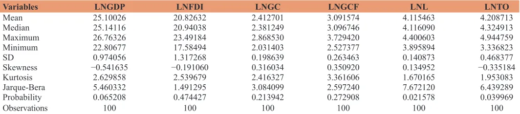
To evaluate the short term and long term association within FDI and economic growth, Cointegration technique and VECM will be applied along these techniques Granger causality test will also be performed in this study. The Cointegration technique was first introduced by (Granger, 1969), then it was further extended and formalized by (Engle and Granger, 1987). In order to perform all estimation techniques the first step is that all variables must be stationary or co-integrated. The steps we have to carry out in this study are unit root will be tested, then co-integration test and in the end Granger causality analysis based on VECM will be applied. Before going to panel data analysis a detailed summary statistics is shown in Table 1 which exhibits the mean, median and standard deviation of all variables; it also shows that all the variables are right-skewed. Kurtosis statistics of all variables illustrate that all the variables are short-tailed or lower peak. A Jarque-Bera test shows that all the variables are normally distributed.

4. EMPIRICAL RESULTS AND

INTERPRETATION

4.1. Panel Unit Root Test

To check the stationarity of the variables, the tests which are used, the Augmented Dickey-Fuller test (ADF) (Dickey and Fuller,

2 Sri Lanka, Pakistan, Philippine, Thailand.

Table 1: Summary statistics of the variables

Variables LNGDP LNFDI LNGC LNGCF LNL LNTO

Mean 25.10026 20.82632 2.412701 3.091574 4.115463 4.208713

Median 25.14116 20.94038 2.381249 3.096746 4.116090 4.324913

Maximum 26.76326 23.49184 2.868530 3.729420 4.400603 4.944759

Minimum 22.80677 17.58494 2.031403 2.527377 3.895894 3.336823

SD 0.974056 1.317268 0.198639 0.263463 0.140873 0.468377

Skewness −0.541635 −0.191060 0.316034 0.350920 0.134952 −0.335184

Kurtosis 2.629858 2.539679 2.416327 3.361606 1.670165 1.953083

Jarque-Bera 5.460332 1.491295 3.084099 2.597240 7.672120 6.439289 Probability 0.065208 0.474427 0.213942 0.272908 0.021578 0.039969

Observations 100 100 100 100 100 100

1981), Phillips-Perron (PP) test (Phillips and Perron, 1988), and Levin, Lin, and Chu (LLC) test (Levin et al., 2002). First of all these tests are performed at level then performed at first difference. Two different models are considered while performing the tests, (1) the model with an intercept (2) the model with intercept and trend. The general form of ADF test which may could be as follows:

With intercept and no trend:

∆Xt a Xt ∆X

i q

i t i t

= + − + +

=

− +

∑

δ 1 δ ε

1 1 (1)

With intercept and trend:

∆X_t a _t X_t ∆X

i q

i t i t

= + + ₋ + +

= − +

∑

β δ ₁ δ ε

1 1

(2)

Where ∆ is first difference, α is constant, β is coefficient of time trend, t is linear time trend, X is the variable under examination, represents the error term, the null hypothesis is X contains unit root, if it is found that the coefficient β is meaningfully different from zero (β ≠ 0) the null hypothesis would be rejected and alternative hypothesis that X doesn’t have a unit root would be accepted.

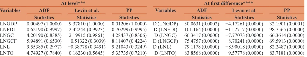
The series is converted into logarithms. Table 2 presents the results from Dickey-Fuller test (ADF), LLC and PP panel unit root tests with lag length of Schwarz Info Criterion. The level results show no variables are stationary in case of Dickey-Fuller test (ADF), LLC test (LLC) and PP, accept the null hypothesis there is a unit root. The first difference results express that all variables are stationary at 5% level and are stationary in the same order I(1). The null hypothesis there is a unit root has been rejected.

4.2. Panel Cointegration Test

When all the variables are integrated in the same order the Cointegration is necessary to be checked. If the Cointegration exists among variables it means long run interrelationship exists among proposed variables. There are two kinds of Cointegration tests. The primary kind is residual (single equation) based Cointegration test and maximum likelihood (system) based Cointegration test. In this study we employed the maximum-likelihood test established by (Johansen, 1988) Panel cointegration maximum likelihood-based test. The null hypothesis is “there is no cointegration.”

The study in hand first employed panel unit root and the results showed that all the proposed variables are stationary at I (1). We already have explained that when all variables are stationary in one order we test Cointegration. The initial point of Johansen Cointegration framework is given as:

1 1 2 2 .

t t t p t p t

y = + A y₋ +A y₋ ……… +A y₋ +

(3)

Where y_t is an n × 1 vector of variables, A denotes the autoregressive matrix, represents the vector of innovations and p represents the lag length. The function can be written as:

∆ = ₋ + ∆ +

= −

−

∑

y_t y_t y

i p

i t i t

Π ₁ Γ

1 1

 (4)

Where,

∏ = − =

− = +

∑

∑

i p

i

j i p

j

A I and A

1 1

� � Γ (5)

If the coefficient matrix Π has shortened rank r < n, then their n × r exists, matrices α and β each with rank r such that Π = αβˈ, where the elements of α are recognized as the analogous adjustment of coefficient in the VECM and β symbolizes the matrix of parameters of the Cointegrating vector. There are two tests under (Fisher/Johansen) test, the first one is called Maximum Eigenvalue test, and the other one is called trace test. Both tests are used to describe the number of Cointegration vectors (r). Both the tests are expressed as:

λtrace λ

i r n

i T

= − −

= +

∑

1 1

log( ) ₍₆₎

λmax = −Tlog(1−λi+1) (7)

Where T is the number of observations and λ is symbolized the values of characteristic roots which are gained from projected matrix. The null hypothesis is that there is r cointegration (r = 0) vectors, the alternative hypothesis is that there is r + 1 cointegration vectors.

Johansen cointegration test is used in this series and Table 3 shows its results. The null hypothesis is no cointegration which

Table 2: Results from panel unit root test

At level*** At first difference****

Variables ADF Levinet al. PP Variables ADF Levinet al. PP

Statistics Statistics Statistics Statistics Statistics Statistics

LNGDP 0.00497 (1.0000) 9.37810 (1.0000) 0.01206 (1.0000) D (LNGDP) 30.0631 (0.0002) −4.17261 (0.0000) 32.1901 (0.0001) LNFDI 0.62190 (0.9997) 2.42244 (0.9923) 0.70299 (0.9995) D (LNFDI) 101.164 (0.0000) −11.2717 (0.0000) 98.7565 (0.0000) LNGC 4.20190 (0.8385) 2.19915 (0.9861) 4.28437 (0.8306) D (LNGC) 66.3417 (0.0000) −7.77073 (0.0000) 66.3614 (0.0000) LNGCF 5.94891 (0.6530) −0.51322 (0.3039) 8.11407 (0.4224) D (LNGCF) 75.4757 (0.0000) −8.70241 (0.0000) 69.5913 (0.0000) LNL 9.55385 (0.2977) −0.38778 (0.3491) 9.21043 (0.3249) D (LNL) 79.1178 (0.0000) −8.90018 (0.0000) 82.2487 (0.0000) LNTO 4.74927 (0.7840) 0.16230 (0.5645) 5.33735 (0.7210) D (LNTO) 83.8568 (0.0000) −9.57778 (0.0000) 83.7181 (0.0000)

is rejected by trace and maximum eigenvalue statistics, the results indicate that two Cointegration equations are found in both trace and maximum eigenvalue test. So here series accept the alternative hypothesis of there is Cointegration. Existence of Cointegration shows the presence of long-run interrelationship within proposed variables.

4.3. The VECM

The vector autoregressive (VAR) model was first introduced by (Sims, 1980). According to him VAR model provide a theory-free methods for the estimation of economic relationship, and it describes the simultaneous relationship between proposed variables. VAR model is utilized to find out the relationship between proposed variables, however the variables which are used in VAR must be stationary. If including variables are non-stationary may create problem, this problem is called spurious relationship. To escape of this problem VECM is a better choice to use. VECM is used to identify the presence of long-run equilibrium interrelationship amongst proposed non-stationary variables. VECM and VAR models are resembles but VECM has an error correction term (ECT) which is a restricted VAR.

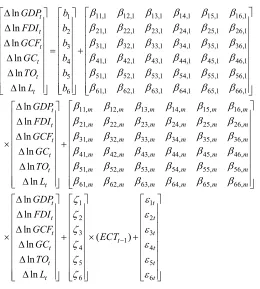
The study in hand is a panel based study, after the estimation of unit root and cointegration test the results show that all the variables are stationary at 1 (I), and cointegration is also exists, so panel VECM is a better model to use. So after finding the long-term interrelation among the variables in Cointegration the next step is to use Granger Causality to define the causality between the proposed variables. After finding the Cointegration within the variables then the dynamic panel causality test established on VECM is developed in equation (8).

11,1 12,1 13,1 14,1 15,1 16,1 1

21,1 22,1 23,1 24,1 25,1 26,1 2

31,1 32,1 33,1 34,1 35,1 36,1 3

41,1 42,1 43,1 44 4 5 6 ln ln ln ln ln ln

β β β β β β

β β β β β β

β β β β β β

β β β β

t t t t t t GDP b FDI b GCF b GC b TO b L b ∆     _∆        ∆    = +     ∆     _∆        ∆        

,1 45,1 46,1 51,1 52,1 53,1 54,1 55,1 56,1 61,1 62,1 63,1 64,1 65,1 66,1

11, 12, 13, 14, 15, 16,

21, 22, 23, 24

ln ln ln ln ln ln β β

β β β β β β

β β β β β β

β β β β β β

β m β m β m β m m m

t

m m m

t t t t t GDP FDI GCF GC TO L                     ∆   _∆    ∆  × + ∆    _∆    ∆    

, 25, 26,

31, 32, 33, 34, 35, 36,

41, 42, 43, 44, 45, 46,

51, 52, 53, 54, 55, 56,

61, 62, 63, 64, 65, 66,

ln ln ln ln ln ln β β

β β β β β β

β β β β β β

β β β β β β

β β β β β β

m m m

m m m m m m

m m m m m m

m m m m m m

m m m m m m

t t t t t t GDP FDI GCF GC TO L                     ∆  ∆  ∆ × _∆   ∆  ∆  1 1 2 2 3 3 1 4 4 5 5 6 6 ( ) ζ ε ζ ε ζ ε ζ ε ζ ε ζ ε t t t t t t t ECT−                     + × +                        _{  } _ _

Where ∆ is the first difference, all the variables are in log form,

ECT_t-1 is the ECT, created from the long term interrelationship. The long term causality is estimated by the significance of coefficient of lagged ECT by using t-statistics. Β_ijs are the short term modification of coefficients, ε_1t, ε_2t, ε_3t, ε_4t, ε_5t and ε_6t, are error terms assumed to be uncorrelated with each other and are normally distributed with mean of zero. The above model is significant only when all variables are stationary at order one I (1) and are cointegrated. On the other hand ECT is detached in the estimation process when the variables are not cointegrated.

The direction of causal interrelationship amongst proposed variables is examined by applying the VECM Granger causality model. In doing so we used the VECM model to detect the causal relationship between GDP, FDI, GCF, GC on, capital and labor which would help policymakers to configure a comprehensive policy to run the economic growth on fast-track in long run.

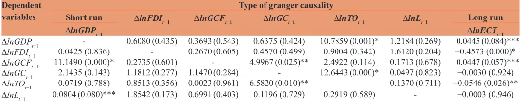
Table 4 represents the results of short term and long term causality relationship. In long-term when ΔlnGDP_t−1 is used by way of dependent variable, the coefficient of lagged ECT is negative and significant which shows that GDP has a coverage tendency to its long term equilibrium in response to changes in its regressors, but one can see there is a comparatively low speed of change to the long term equilibrium. Negative ECT shows that there is a long term Granger causality running from FDI, GCF, GC, TO and labor to GDP. The other long term causality relationship is when ΔlnFDI_t−1 is used by way of dependent variable, the lagged ECT is negative and statistically important, which shows that GDP, GCF, GC, TO, and labor are Granger cause to FDI in the long term. There is another long term causality relationship when ΔlnGCF_t−1 is used in place of dependent variable, the lagged ECT is important and negative, this shows that GDP, FDI, GC, TO and labor Granger cause to GCF in the long term. There is another Granger causal relationship when ΔlnTO_t−1 is used in place of dependent variable the lagged ECT is statistically important and negative which shows that GDP, FDI, GCF, GC and labor Granger cause TO in the long term.

The short-term results demonstrate that there is a bidirectional causal relationship between GC and TO [lnGC↔lnTO]. A unidirectional causal interrelationship exists which is running from TO to GDP [lnTO→lnGDP], another unidirectional causal relationship is found running from GC to GCF [lnGC→lnGCF] and GDP to GCF [lnGDP→lnGCF]. We find the existence of another unidirectional causal relationship running from GDP to labor [lnGDP→lnL].

5. CONCLUSION

Factual outcomes show that all the included variables are integrated at I(1), that is proved by the panel unit root. The Cointegration results illustrate that there is a long-term interrelationship among proposed variables. The study applied VECM, the observed findings show that there is a positive and statistically noteworthy long-term relationship amongst FDI and GDP. This suggests the selected Asian countries in this study that if they increase in FDI inflow it cause increase in GDP.

The importance of the study is to provide information, to the countries which are included in this study that will work as a guideline to the policy makers for the implementation of short-run and long-run policies and development goals. First, these Asia countries should provide incentives to attract FDI inflow. Second, the lawful framework regulating FDI in the Asian region should be empowered. This will cause a favorable investment environment in the Asian region and will attract FDI in the region.

REFERENCES

Aitken, B.J., Harrison, A.E. (1999), Do domestic firms benefit from direct foreign investment? Evidence from Venezuela. American Economic Review, 89(3), 605-618.

Asheghian, P. (2004), Determinants of economic growth in the United

States: The role of foreign direct investment. International Trade Journal, 18, 63-83.

Basu, P., Chakraborty, C., Reagle, D. (2003), Liberalization, FDI, and growth in developing countries: A panel cointegration approach. Economic Inquiry, 41(3), 510-516.

Basu, P., Guariglia, A. (2007), Foreign direct investment, inequality, and growth. Journal of Macroeconomics, 29(4), 824-839.

Belloumi, M. (2014), The relationship between trade, FDI and economic growth in Tunisia: An application of the autoregressive distributed lag model. Economic Systems, 38(2), 269-287.

Bevan, A., Estrin, S. (2004), The determinants of foreign direct investment in transition economies. Journal of Comparative Economics, 32, 775-787.

Billington, N.M. (1999), The location of foreign direct investment: An empirical analysis. Applied Economics, 31, 65-76.

Borensztein, E., De Gregorio, J., Lee, J.W. (1998), How does foreign

direct investment affect economic growth. Journal of International

Economics, 45(1), 115-135.

Brems, H. (1970), A growth model of international direct investment. American Economic Review, 60, 320-331.

Carkovic, M.V., Levine, R. (2005), Does Foreign Direct Investment Accelerate Economic Growth? Does Foreign Direct Investment Promote Development?. Washington, DC: Institute of International Economics. p195-222.

Caselli, F., Esquivel, G., Lefort, F. (1996), Reopening the convergence debate: A new look at cross-country growth empirics. Journal of Economic Growth, 1(3), 363-389.

Cavusgil, S.T., Knight, G., Riesenberger, J. (2008), International Business. Strategy. Management Ans the New Realities. Available from: https://www.pearsonhighered.com/product/Cavusgil- International-Business-Strategy-Management-and-the-New-Realities/9780131738607.html.

Daniels, J.D., Radebaugh, L.H., Daniel P, Sullivan. (2004). International Business: Environments and operations. Long Range Planning. Reading, MA: Addison-Wesely.

De Gregorio, J. (2003), The Role of Foreign Direct Investment and Natural Resources in Economic Development. Working Papers of the Bank of Chile. p. 1-26. Available from: http://www.dialnet.unirioja.es/ servlet/articulo?codigo=965310.

De Mello, L.R. (1999), Foreign Direct Investment-Led Growth: Evidence from Time Series and Panel Data. Vol. 51. Oxford Economic Papers. p133-151.

De Mello, L.R.Jr. (1997), Foreign direct investment in developing countries and growth : A selective survey. Journal of Development Studies, 34(1), 1-34.

Dickey, B.Y.D.A., Fuller, W.A. (1981), Likelihood ratio statistics for

autoregressive time series with a unit root. Journal of Econometric

Society, 49(4), 1057-1072.

Engle, R.F., Granger, C.W.J. (1987), Co-integration and error correction: Representation, estimation, and testing. Econometrica, 55(2), 251-276. Fang, Q., Liu, Y. (2007), Empirical analysis : Business cycles and inward

Table 3: Results from panel cointegration test

Hypotheses No. Hypotheses Fisher Stat.* Prob. Fisher Stat.* Prob.

H0 H1 From trace test From max-eigen test

r=0 r≥1 113.5 0.0000 66.20 0.0000

r≤1 r≥2 56.33 0.0000 36.18 0.0000

r≤2 r≥3 26.89 0.0007 14.36 0.0729

r≤3 r≥4 17.31 0.0270 11.70 0.1652

r≤4 r≥5 11.38 0.1810 10.79 0.2141

r≤5 r≥6 8.874 0.3530 8.874 0.3530

Probabilities are computed using asymptotic Chi-square distribution. Null hypothesis: There is no cointegration.

Table 4: The results of short run and long run panel VECM granger causality analysis

Dependent

variables Short run ΔlnFDI_t−1 ΔlnGCF_t−1 Type of granger causalityΔlnGCt−1 ΔlnTOt−1 ΔlnLt−1 Long run

ΔlnGDPt−1 ΔlnECTt−1

ΔlnGDP_t−1 - 0.6080 (0.435) 0.3693 (0.543) 0.6375 (0.424) 10.7859 (0.001)* 1.2184 (0.269) −0.0445 (0.084)***

ΔlnFDI_t−1 0.0425 (0.836) - 0.2670 (0.605) 0.4570 (0.499) 0.9004 (0.342) 1.6120 (0.204) −0.4573 (0.000)*

ΔlnGCF_t−1 11.1490 (0.000)* 0.2735 (0.601) - 4.9967 (0.025)** 2.4922 (0.114) 0.1713 (0.678) −0.0447 (0.057)***

ΔlnGC_t−1 2.1435 (0.143) 1.1812 (0.277) 1.1470 (0.284) - 12.6443 (0.000)* 0.0497 (0.823) −0.0030 (0.924)

ΔlnTO_t−1 0.0719 (0.788) 0.8513 (0.356) 0.0023 (0.961) 6.5820 (0.010)** - 0.1370 (0.711) −0.0546 (0.026)**

ΔlnL_t−1 0.0804 (0.080)*** 1.8542 (0.173) 0.6991 (0.403) 0.1196 (0.729) 0.2919 (0.589) - −0.0003 (0.946)

*,_{** and ***show significance at 1%, 5% and 10% levels respectively. VECM: Vector error correction model, GDP: Gross domestic product, FDI: Foreign direct investment, GCF: Gross}

FDI in China Qiyun Fang, Yao Liu School of Economics, Huazhong University of Science and Technology. Journal American Sciences, Applied Publications, Science, 4(10), 802-806.

Fosfuri, A., Motta, M., Rønde, T. (2001), Foreign direct investment and spillovers through workers’ mobility. Journal of International Economics, 53(1), 205-222.

Ghirmay, T. (2004), Financial development and economic growth in Sub-Saharan African Countries: Evidence from time series analysis. African Development Review, 16(3), 415-432.

Glass, A.J., Saggi, K. (2002), Multinational firms and technology transfer. Scandinavian Journal of Economics, 104(4), 495-513.

Granger, C.W.J. (1969). Investigating causal relations by econometric models and cross-apectral methods. The Econometric Society, 37(3), 424-438. Available from: http://www.jstor.org/stable/1912791. Günther, J. (2002), FDI as a multiplier of modern technology in Hungarian

industry. Intereconomics, 37(5), 263-269.

Johansen, S. (1988), Statistical analysis of cointegration vectors. Journal of Economic Dynamics and Control, 12(2-3), 231-254.

Johansen, S., Juselius, K. (1990). Maximum likelihood estimation and

inference on cointegration with applications to the demand for

money. Oxford Bulletin of Economics and Statistics, 52(2), 169-210. Karimi, M.S., Yusop, Z. (2008), FDI and Economic Growth in Malaysia.

Business, 8225. Retrieved From: https://mpra.ub.uni-muenchen. de/14999/1/ MPRA _paper_14999.pdf.

Kornecki, L., Raghavan, V. (2011), Inward FDI stock and growth in central and eastern Europe. The International Trade Journal, 25(5), 539-557. Levin, A., Lin, C.F., Chu, C.S.J. (2002), Unit root tests in panel data:

Asymptotic and finite-sample properties. Journal of Econometrics, 108(1), 1-24.

Li, X., Liu, X. (2005), Foreign direct investment and economic growth: An increasingly endogenous relationship. World Development, 33(3), 393-407.

Lipsey, R. (2002), Home and host country effects of FDI. The European Journal of Health Economics, 8(4), 305-312.

Liu, X., Shu, C., Sinclair, P. (2009), Trade, foreign direct investment and economic growth in Asian economies Trade, foreign direct investment and economic growth in Asian economies, 6846. Applied Economics, 41(13), 1603-1612.

Mah, J.S. (2010), Foreign direct investment inflows and economic growth of China. Journal of Policy Modeling, 32(1), 155-158.

Nair-Reichert, U., Weinhold, D. (2001), Causality tests for cross-country panels: A new look at FDI and economic growth in developing countries. Oxford Bulletin of Economics and Statistics, 2(63), 153-172.

Neto, G., José, F. (2012), Financial globalization, convergence

and growth : The role of foreign direct investment. Journal of

International Money and Finance, 37, 1-38.

Odhiambo, N.M. (2009), Energy consumption and economic growth nexus in Tanzania: An ARDL bounds testing approach. Energy Policy, 37(2), 617-622.

Omer, M.S., Yao, L. (2011), Empirical analysis of the relationships between inward FDI and business cycles in Malaysia. Modern Applied Science, 5(3), 157-163.

Phillips, P., Perron, P. (1988), Testing for a unit root in time series regressions. Biometrika, 75(2), 335-346.

Rodrick, D. (1999), The New Global Economy and Developing Countries. Washington, DC: Overseas Development Council.

Salehizadeh, M. (2005), Foreign direct investment inflows and the US economy: An empirical analysis. Economic Issues, 10, 29-50. Sharahili, Y., Liu, Y. (2008), Empirical analysis II: Business cycles

and inward FDI in China. Journal, American Sciences, Applied Publications, Science, 5(10), 1409-1414.

Sims, C.A. (1980), Macroeconomics and Reality. The Econometric Society, 48(1), 1-48. Available from: http://www.jstor.org/

stable/1912017.

Sothan, S. (2017), Causality between foreign direct investment and

economic growth for Cambodia. Cogent Economics and Finance,

5(1), 1277860.

Vu, T.B. (2008), Foreign direct investment and endogenous growth

in Vietnam Foreign direct investment and endogenous growth in

Vietnam, 6846. Applied Economics, 40(9), 1165-1173.

Vu, T.B., Noy, I. (2009), Sectoral analysis of foreign direct investment and

growth in the developed countries. Journal of International Financial

Markets, Institutions and Money, 19(2), 402-413.

Wang, J.Y., Blomström, M. (1992), Foreign investment and technology transfer. European Economic Review, 36(1), 137-155.