Copyright © 2014 IJECCE, All right reserved
Radar Image Texture Classification based on Gabor
Filter Bank
Mbainaibeye Jérôme, Olfa Marrakchi Charfi
Abstract – The aim of this paper is to design and develop a filter bank for the detection and classification of radar image texture with 4.6m resolution obtained by airborne synthetic Aperture Radar.The textures of this kind of images are more correlated and contain forms with random disposition. The design and the developing of the filter bank is based on Gabor filter. We have elaborated a set of filters applied to each set of feature texture allowing its identification and enhancement in comparison with other textures. The filter bank which we have elaborated is represented by a combination of different texture filters. After processing, the selected filter bank is the filter bank which allows the identification of all the textures of an image with a significant identification rate. This developed filter is applied to radar image and the obtained results are compared with those obtained by using filter banks issue from the generalized Gaussian models (GGM). We have shown that Gabor filter developed in this work gives the classification rate greater than the results obtained by Generalized Gaussian model. The main contribution of this work is the generation of the filter banks able to give an optimal filter bank for a given texture and in particular for radar image textures.
Keywords – Radar Image, Filter Bank, Gabor Filtering, Texture, Identification Rate, Classification Process.
I.
I
NTRODUCTIONIMAGEanalysis consists to extract some characteristic proprieties and to allow the parametric representation. The parametric extraction is often the first procedure of the decision step.
The remote sensing offers, with a lot of satellite equipments available today, more and more images, data and information which may not be accessible from the earth. Remote sensing becomes an important topic because it is an excellent tool for decision and is necessary for the terrestrial resources. The analysis and interpretation of these images constitute an intensive scientific study and research activities through the world. The information interpretation in the natural environment is not an easy task. In fact, the natural textures are more irregular and the classical modeling such as statistical methods and orthogonal transforms are not appropriate because these techniques cannot give the desired precision.
In recent decade, spatio-frequential methods are more and more used because psycho physiological study results operated in human visual system show that the nervous system processes the images by using frequential analysis. These studies establish that image is decomposed in many scales relative to different frequential channels. This paper presents a method for texture identification based on the Gabor filter bank. The remaining of this paper is structured as following: in the section II, we present the state of the art and the classical texture analysis. Few literatures on Gabor filtering and Generalized Gaussian
Model are presented in section III. Our contribution consisting to develop a procedure for the application of Gabor filtering on radar texture image is presented in section IV. Section V presents the simulation and results. Finally section VI presents conclusion and perspectives of this work.
II.
S
TATE OF THEA
RTA. Few elements about textures
Texture may be defined by an image area which presents homogeneity of its characteristics; it may be also defined as a group of primitives presenting variable form and size which have particular spatial organization [1][2]. There exist two types of textures:
- The macro textures which have a regular aspect consisting in periodical forms for which the spatial position obeys to a precisely law;
- The micro textures presenting the microscopic primitives for which the spatial distribution is a random process. Despite their random spatial distributions, they are homogenous in its environment [3].
Brodatz has established a catalogue of texture [4] and this catalogue is today a most popular of the texture data set. The figure 1 and figure 2 show Brodatz textures having one scale and multiple scales respectively.
Fig.1. Brodatz textures with one scale
Fig.2. Brodatz textures with multiple scales
B. Texture analysis
Globally, there is a diversity of approaches used to describe or identify textures [5]. Some approaches are based on stochastic models or on the linear prediction. Other approaches are based on statistical analysis or on the orthogonal transforms.
Copyright © 2014 IJECCE, All right reserved
1)
Statistical methods
They are based on quantitative evaluation of the grey scales or on other primitives. These methods study the relationship between a pixel and its neighbors and define discriminate parameters of the texture using statistic tools. In general, these methods are used for the characterization of fine textures having no apparent regularity [14][15]. Matrix of grey scales co-occurrences is the distribution of the nature [16].
2)
Geometric methods
They are concerned by structural analysis based on the identification of one ore many features and their spatial repartition. The result depends of the geometric properties of primitives and their spatial constraints [15]
3)
Methods based on a model
The objective of these methods is to obtain a model which may be considered as a generator of the texture [17]. The parameters of this model are used for the characterization or the synthesis of a texture. The Markov fields belong to these methods.
4)
Frequential methods
They consist to analysis the texture in the spectrum or the repetition of features explained by the apparition of specific frequencies. One distinguishes three types of filtering: spatial filtering, Gabor filtering and wavelet transform. Among these filtering types, the Gabor filtering has demonstrated its performance in texture analysis and description [18][19]. The Gabor filters are particularly a power tool for the texture classification [19][20]. Among the spatio-frequential filtering methods, the Gabor filtering meet a great and particular attention in scientific research activities [6][7].
The interpretation of the information in the natural environment is one of the most important activities of human visual system but the modeling of this task is not easy. The natural textures are so irregular that their modeling by classical methods such as statistical or orthogonal transforms cannot give the desired results [8][9]. It is necessary to use methods able to approximately accomplish the human visual system procedure in image analysis [10]. The Gabor filtering uses redundancy within image data to represent an explain each pixel; this redundancy used is the main reason that introduces a delay in the texture processing (the rapidity is not optimal) but the Gabor filtering can give the desired result [11] and it is very important because the texture describing and identification don’t requires a necessary real time processing and the rapidity is not a requirement.
III.
F
EWE
LEMENTS ONG
ABORF
ILTERING ANDG
ENERALIZEDG
AUSSIANM
ODELA.
Gabor filtering
In image analysis, when there are multiple local orientations, methods based on filter bank are often used. These methods consist to search the orientation corresponding to the maximum of filter bank where each filter is the result of the rotation of a basis filter called also the mother filter.
In this work, we use the Gabor filter with add symmetry and for which the orientation is zero degree. The Gabor filter may be considered as a complex frequency modulated by the Gaussian function [1] and the pass-band filter. For signal processing, this filter is defined by equation (1):
x x
j f x
g x
x x
b exp 2 0
2 exp 2
1 2
(1)
Where x is the standard deviation of the Gaussian and
0
x
f is the central frequency. The selectivity of this band pass filter may be controlled by x because bigger isx, high is the selectivity.
In image processing, this filter is considered in its bi-dimensional form defined by equation (2) [21]:
x y x y
j
f x f y
g x y
y x y
x
b exp 2 0 0
2 2 exp 2 1 , 2 2 (2) It is possible to simplify the equation (2) by considering the polar representation where 0 2 2
0
0 y
x f
f
f will be the central frequency in bi-dimensional form and
0 0 tan x y f f a
will be the filter orientation with02 Finally, the basis form of the Gabor filter may be expressed using equation (3):
exp
2
' '
2 2 exp 2 1 , 0 2 2 y x f j x x y x g y x y x
b
(3)
Where
y x y x cos sin sin cos ' '
In texture analysis, we have needed to localize information both in spatial domain for characterizing the orientations of the primitives and in frequential domain for obtaining the grey scales variation which can indicate the separation between features. In this context, the Gabor filter is the solution [22] [23].
The best simultaneous localization in spatial and frequential domain may by operated by the Gabor filtering applying a cosine filter type having a certain direction modulated by a Gaussian window [24][25]. In this work, we have radar image which is the real data, we have needed the real form of the Gabor filter defined by equation (4):
x y x y
f
x y
g
y x y
x
b
2 2 cos2 0
2 2 exp 2 1 ,
(4)
To obtain different orientation, we need to operate a rotation of the coordinate axis using equation (5):
i i
y i x i y x i i
b f x y
y x y
x
g
2 2 cos2 0
2 2 exp 2 1 ,
(5)
Where
y x y x i i i i i î cos sin sin cos and 0 0 0 0 i for i for i
Copyright © 2014 IJECCE, All right reserved resulting filter is the sum of the basis filters in each
direction defined by equation (6):
gb xi yi
g , (6)
B.
Generalized Gaussian Model
1)
Discreet Wavelet Transform
Multi-resolution analysis is a formal and general approach for constructing wavelet orthogonal basis. It is based on the principle according to which the signal can be represented by a set of approximation and details coefficients. In practice, dyadic wavelet decomposition is carried out by filtering and sub-sampling, using “Quadrature Mirror Filters” HF and LF due to Mallat theory [26]. For image or 2D signal, the decomposition is achieved by applying separable 1D filters HF and LF (see figure 3) where LF and HF design Low Frequency and High Frequency respectively.
2 , 1 1 , 2 1 3 2 , 1 1 , 2 1 2 2 , 1 1 , 2 1 1 2 , 1 1 , 2 1 n y x n n y x n n y x n n y x n L g g D L h g D L g h D L h h L (7)Where (*) is a convolution product, Ln is an approximation image and Dn1,Dn2, Dn3 are details images at the n-th scale, h and g are the filters (respectively HF and LF) in equation (7) and are called Quadratic Mirror Filters, they satisfy the complementarily criterion (8):
1 h(1 m) )m (
g 1m (8)
At any scale, the approximation image is also decomposed in approximation and details subbands. Details subbands coefficients correspond to wavelet coefficients of the signal at a given scale. However, the approximation subband represents the low frequencies information; on the other hand, detail subbands provide the high frequencies information. So, if n is the number of decomposition levels, we get 3n+1 different subbands describing the image.
Fig.3. DWT image decomposition
2)
Textural signatures
(a) Energy signature and L1 norm
According to Wouwer, a number of synthetic textures can be characterized by the energy signature (equation 9) as well as by L1 norm called « average deviation (MDni
) » (equation 10).
2 k , j k j ni
ni (D (b ,b ))
M 1
E
(9)
k , j k j nini D (b ,b )
M 1
MD (10)
WhereDni(bj,bk) is the value of wavelet coefficient of the detail subband i at the pixel position(bj,bk); M is the total number of image pixels; n is the decomposition level.
(b) Generalized Gaussian model applying to texture
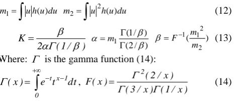
According to Mallat, texture histogram modelling in detail subband images by a set of exponential function under a generalized Gaussian law (equation 11) and extracting the signatures of the textures (equation 9), (equation 10) from these models (equation 6) are possible (the translation invariance should be ensured). ) u ( Ke ) u (
h (11)
Where: is the parameter which can modify the decrease of the histogram peak (for 2, the histogram is a Gaussian distribution);
is the histogram width (represents the variance); Kis a constant which ensures
h(u)du1.The parameters , and K (13) may be used to calculate the 1st and 2sd order moments equivalent respectively to m1 and m2 values which indicate the energy
distribution for each subband (equation 12).
uhudu
m1 ( ) m u h(u)du 2
2
(12)) / 1 ( 2 K
) / 2 ( ) / 1 ( 1 m ( )
2 2 1 1 m m F
(13)
Where:
is the gamma function (14):
0 1 x t dt t e ) x ( , ) x / 1 ( ) x / 3 ( ) x / 2 ( ) x ( F 2 (14)Indeed, the function h represents the energy distribution in the subbands and m1 and m2 represent respectively Eni
and MDni values of the subbands (equation 9), (equation 10). However, the texture can be characterized by a signature vector V which is composed of 6 elements representing, respectively, the energy E in the three details subbands: horizontal details (DH), vertical details (DV), diagonal details (DD)) and L1 norm (MD) in the three details subbands (equation 15).
V(EDH,EDV,EDD,MDDH,MDDV,MDDD)T (15)
IV.
P
ROCEDURE FORA
PPLICATION OFG
ABORF
ILTER TOR
ADARI
MAGECopyright © 2014 IJECCE, All right reserved
0
f to extract, the standard deviations xandy. For the user of Gabor filter, only two parameters have to be chosen: the direction number (orientation) and the number of scales (frequencies). It is also necessary to choose other parameters, such as the analysis window size and this last will be presented in the next under section.
A.
Choice of orientation
In an image point or pixel, the orientation corresponds to the axis which well characterizes this image in the human visual system consideration [27]. Figure 4 shows an example of synthetic texture where we can see a unique orientation corresponding to an angle comparing to an arbitrary reference.
Fig.4. Synthetic texture characterized by an orientation equal to 30°.
In the presence of multiple local orientations, it is important to search an orientation corresponding to the maximum of the filter response.
B.
Choice of filtering frequency
To obtain the best results of Gabor filtering, appropriate choice of frequency is important. The choice of the frequency may be done by the response to the following question: until what low frequencies the image must be decomposed? In the other terms, how many scale levels the image must be decomposed? As the response to this question, the scale level number depends on the size of the image and on the nature of texture. For the nature of texture, there exist two categories [12]: some textures have one scale, other textures have multiple scales.
C.
Choice of the window size
The size of analysis window is an important parameter but it is also one of the delicate choice of the texture analysis (see figure 5).
Fig.5. Influence of the choice of the analysis window size on the image texture
In the figure 5, for example window A can determine the characteristic properties of a tile and permits to distinguish the clear tiles from the dark tiles; window B can give the average properties but cannot distinguish the clear tiles from the dark tiles.
D.
Choice of standard deviations
The standard deviations x and ycorrespond to the width of the Gaussian function in x and y directions respectively. The choice of these parameters must be done appropriately if we want to extract the information in the image texture. If all the primitives have the same size, the Gaussian function is isotropic and we can choicexy. High is the value of, significant is the low frequencies of the filtered image. Low is the value of , the details of textures in the filtered image well appears.
However, there exist a relationship between the size of the analysis window and the width of the Gaussian function (). The size of the analysis window must be significant to adapt the Gaussian function [28].
V.
S
IMULATIONS AND RESULTSA.
Block scheme of filtering
In figure 6, we present the procedure developed for Gabor filtering.
Copyright © 2014 IJECCE, All right reserved In texture analysis, it is not necessary to use color
image; grey scale image is sufficient to describe the texture. This scheme shows that for each image, the four parameters f0, θ, σx, and σy have to be chosen
appropriately for the application of Gabor filtering. The approach developed in this work, shown en in figure 6, is based on a multichannel filtering. It consists to decompose, by filtering, the image in a set of images containing the spatial characteristics at different scales. Furthermore, the original image is decomposed on different planes corresponding to different frequential channels. Each of these images captures the textural characteristics appearing in a narrow spatial frequency band and orientation. This approach has the advantage to exploit the spatial interactions between pixels of neighboring at different scales.
After filtering, we select the filters able to offer the capacity for efficiently detecting the texture motives.
B.
Data sets
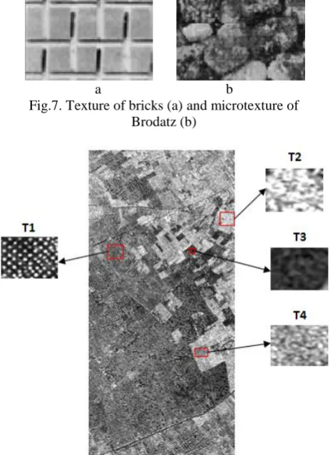
To evaluate the developed filter, we use the texture data set presented in the figure 7 and figure 8.
a b
Fig.7. Texture of bricks (a)and microtexture of Brodatz (b)
Fig.8. Four textures T1, T2, T3 in airborne synthetic aperture radar: T1 is an olive tree, T2 is a built, T3 is a
bare ground, and T4 is sparse vegetation.
C.
Results of simulations
We show the results obtained on different test images in this work.
1)
Results for bricks
The figures 9 to 12 show the results of Gabor filtering of the brick texture. The size of the analysis window is 9x9; we vary the three other parameters which are the orientation θ, the frequency f0 and the standard deviation.
The Gabor filters frequency f0 varies from 0.02 to 0.47 and
the standard deviation sigma varies from 0.3 to 1.5. The orientation θ have taken the following values: 0, 5π/8, π/4, and π/2.
Fig.9. Filtered sequences in function of the frequency f0
and the standard deviation σ for θ = 0.
Fig.10. Filtered sequences in function of the frequency f0
and the standard deviation σ for θ = π/2
Fig.11. Filtered sequences in function of the frequency f0
and the standard deviation σ for θ = π/4
Fig.12. Filtered sequences in function of the frequency f0
Copyright © 2014 IJECCE, All right reserved From figures 9 to 12, we may see that the filtered
images have a background globally blurry corresponding to the regions which have no response in the researched direction.
However, we may see the white and dark zones on the edge of brick textures corresponding to the regions which have a significant response in the researched direction. We can conclude that to extract the pertinent information both in space (direction) and in frequency (related to the textures) or the texture primitives of the brick, it is sufficient to detect its edges. This may be possible by using:
- The orientation filters which have two values: 0 and π/2; it means that if the filter and the texture have not the same direction, (edges of the brick in this case), the filter cannot give the response;
- The frequencies which can give the best performances can also efficiently reveal the texture primitives. These frequencies are [0.02; 0.07; 0.22; 0.22; 0.27; 0.37; 0.42]. For the standard deviation σ, we may see that big is its value, more smoothed is the filtered image and the obtained image is blurry.
These results show that a bank of 12 Gabor filters (6 frequencies and 2 directions) isotopic (σx = σy = 0.3) is
able to describe the textures present in this image.
2)
Results for the micro-texture of Brodatz
We consider now a complex texture presenting the primitives randomly distributed in the image such that shown in the figure 13.
Fig.13. Micro-texture of Brodatz
The micro-texture with different scales presents a multiple orientations. It is necessary to have many frequencies and orientations for the features filtering. We have chosen 15x15 as the size of the analysis window, the standard deviations are σx = 1, σy = 0.5, the orientation has
taken the following values: 0, π/8, π/6, and π/2.
For each orientation, many tests allow us to choose these values of frequency f0: 0.03; 0.05; 0.1; and 1. We
have then developed a filter bank having four frequencies and four orientations, so we have obtained a bank of 16 filters. The figure 14 shows the obtained results for micro-texture of Brodatz.
The different parameters (central frequency f0, σ, θ)
used in this filtering (see figure 14) have been experimentally chosen. The optimization method of these choices is based on visual evaluation of the results. We may conclude that using this type of spectral analysis, we can characterize and describe the primitives of the textures. This observation justifies the choiceof this type of filtering for multispectral images and in particular the radar images analysis.
Θ = 0, f0 = 0.03 Θ = 0, f0 = 0.05 Θ = 0, f0 = 0.1 Θ = 0, f0 = 1
Θ = π/8, f0 = 0.03 Θ = π/8, f0 = 0.05 Θ = π/8, f0 = 0.1 Θ = π/8, f0 = 1
Θ = π/6, f0 = 0.03 Θ = π/6, f0 = 0.05 Θ = π/6, f0 = 0.1 Θ = π/6, f0 = 1
Θ = π/2, f0 = 0.03 Θ = π/2, f0 = 0.05 Θ = π/2, f0 = 0.1 Θ = π/2, f0 = 1
Fig.14. Filtering of Brodatz micro-texture by Gabor filter with different frequencies and different directions. The
size of analysis window is 15x15.
3)
Result for radar image
The radar image is composed of four texture sub-images: olive tree, built, bare ground and sparse vegetation. The figures 15 to 22 show the obtained results.
(a) Olive tree
Fig.15. Filtered sequences of the olive tree texture f0 є [0,01 ; 0,15], θ = 0°, the analysis window size is 3x3.
Copyright © 2014 IJECCE, All right reserved
(b) Frame
Fig.17. Filtered sequences of the builds texture f0 є [0,01 ; 0,15], θ = 0°, the analysis window size is 3x3
.
Fig.18. Filtered sequences of the frames texture f0 є [0,15 ; 0,5], θ = 0°, the analysis window size is 3x3
(c) Sparse vegetation
Fig.19. Filtered sequences of the sparse vegetation texture f0 є [0,01 ; 0,15], θ = 0°, the analysis window size is 3x3
Fig.20. Filtered sequences of the sparse vegetation texture f0 є [0,15 ; 0,5], θ = 0°, the analysis window size is 3x3
(d) Bare ground
Fig.21. Filtered sequences of the bare ground texture f0 є [0,01 ; 0,15], θ = 0°, the analysis window size is 3x3
Fig.22. Filtered sequences of the bare ground texture f0 є [0,15 ; 0,5], θ = 0°, the analysis window size is 3x3
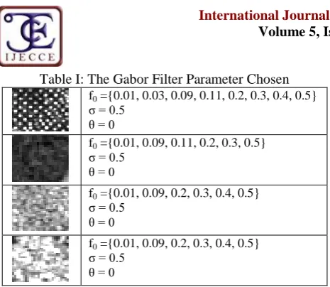
Copyright © 2014 IJECCE, All right reserved Table I: The Gabor Filter Parameter Chosen
f0 ={0.01, 0.03, 0.09, 0.11, 0.2, 0.3, 0.4, 0.5}
σ = 0.5 θ = 0
f0 ={0.01, 0.09, 0.11, 0.2, 0.3, 0.5}
σ = 0.5 θ = 0
f0 ={0.01, 0.09, 0.2, 0.3, 0.4, 0.5}
σ = 0.5 θ = 0
f0 ={0.01, 0.09, 0.2, 0.3, 0.4, 0.5}
σ = 0.5 θ = 0
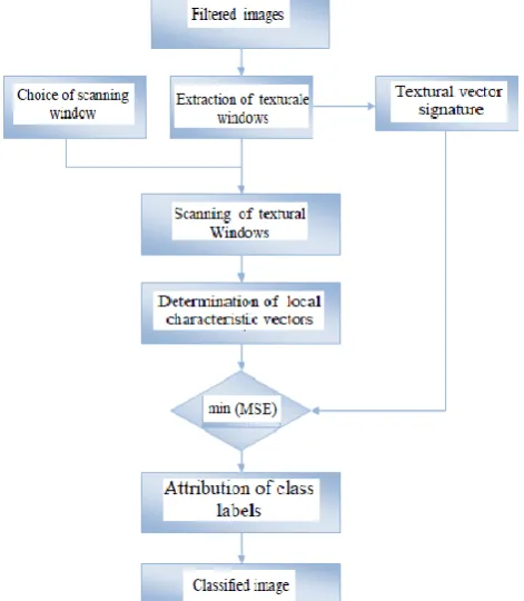
There exist in the literature many methods and models for the characterization of texture by textural signatures [29]. Among these characteristics, we can note the orientation and the frequency. It concerns in particular interactions between each pixel and its neighboring since the texture is defined by the luminosity variations in the neighboring and by the symmetry. Our goal in this work is to operate on the digital representation of the texture, it is necessary to obtain the measures in a vector representation. These measures correspond to the extraction of the texture characteristics. Figure 23 shows the general scheme for the characterization of the texture based on the vectors of the statistic characteristics.
Fig.23. General scheme for the texture characterization based on the characteristic vectors
The image texture Tj, is represented by a set of vectors
Cpq, each vector is associated to the pixel neighboring where, (p, q) is the spatial position of the pixel and [P x Q] is the image size. The set of the K measures (filtered sequences), defines the vector size.
We operate the characteristics extraction after the filtering of the texture. This operation is described in the figure 24 where an energy measurement is accomplished.
Fig.24. Extraction process of textural characteristics after filtering.
It is possible to characterize some textures by the L1 [9] norm which can define the distribution of the pixel average value of filtered images using equations 16 and 17:
Q P
q p I E
P
i Q
j ij
* ,
1 1 2
(16)
Q P
q p I V
P
i Q
j ij
* , 1 1
(17)
Where:
Eij defines the energy of the Gabor filter coefficients of texture i after filtering by the Gabor filter of frequency j;
Vij defines the L1 norm obtained from the output of Gabor filter of frequency j.
The characteristic vector of each texture Ti of the radar image contains the values of Eij and Vij. For example, if we use a bank of four filters, the characteristic vector will have the form defined in equation 18:
Ci
Ei1,Ei2,Ei3,Ei4,Vi1,Vi2,Vi3,Vi4
(18)Ei1 represents the energy of the Gabor filter coefficients
for the first frequency of the texture i.
The textural signatures are determined for all the textures of the radar image. The selected textural signatures are those which have the best results in terms of texture classification. Table II presents the selected textural signatures.
Table II: Example ofTexturalSignatures of RadarImage f0 = [ 0.01, 0.09, 0.1, 0.9] E1
x 103
E2 x 103
E3 x 103
E4 x 103
V1 x 103
V2 x 103
V3 x 103
V4 x 103
T1 2.07 2.07 11.87 2.07 38.45 38.45 92.89 38.45
T2 7.33 7.33 42.57 7.33 83.41 83.41 201.33 83.41
T3 0.52 0.52 3.06 0.52 21.84 21.84 52.83 21.84
T4 4.83 4.83 27.92 4.83 68.30 68.30 164.30 68.30
D.
Principle of classification
In general, classification consists to estimate the membership of a pixel to a given class in function of a certain criterion. There are two types of classification [30] [31]:
- Supervised classification based on the knowledge of the number and the type of the class to identify;
Copyright © 2014 IJECCE, All right reserved The objective of this work is the classification of the
different zones of radar image and we adopt the method based on the study followed by the classification.
The study phase corresponds to the extraction of characteristic attributes from the image; it consists, for a given class, to concatenate all the regions included in the study zones and study the repartition of their vectors associated in the space state.
The classification phase corresponds to use the precedent extracted attributes to obtain the initial objective. The classifier receives at the input the parameters calculated in an observation window and furnishes, at the output, an indication of the texture class [32].
In the texture analysis by the Gabor filter method, we can use either the output values of the filter directly or the local statistics [33][34]. In this work, we have adopted the supervised classification based on the minimization of the mean square error (MSE) between the local statistics calculated in the observation window and the textural signature using equation 19:
24 4 2 3 3 2 2 2 2 1
1 i i i i i i i
i E e E e E e E
e
MSE
24 4 2 3 3 2 2 2 2 1
1 i i i i i i i
i V v V v V v V
v
(19)
With:
4 3 2 1 4 3 2
1, i , i , i , i , i , i , i i E E E V V V V
E are the signatures of the
texture Ti considered as the energy value in L1 norm for the four filtered images.
4 3 2 1, i , i , i i e e e
e are the local energies (that are function of the scanning window) calculated using equation 16 and
4 3 2 1, i , i , i i v v v
v are the local signatures of the texture Ti in L1 norm calculated using equation 17 obtained from the four filtered images.
Fig.25. Our developed classification method
The textural characteristic vector (or textural signature) which gives the minimum distance will attribute to the window the associated class. The procedure consists to determine, in the first step, the characteristic parameters of the textural windows extracted from the images resulted from the decomposition of the original image in different frequential channels. In the second step, we scan the decomposed images using the sampling window (for which the size is (k x k)) and we determinate the local characteristic vectors which will allow us to calculate the MSE. The textural signature that gives the minimal distance will attribute to the window the associated class. The figure 25 describes our method.
1)
Evaluation criterion of classification
The classification results are evaluated in terms of identification rate id
T of textural windows based on thelabels image defined by equation 20:
c
i s s
s s id
i I T T p
T T i I p T
1 /
/ 100
(20)
With:
c is the number of the considered class;
Is the label of the pixel s;
I i T T
p s / s and p
TTs/Isi
are the conditional probabilities where s designs the pixel, I designs the class and T designs the texture.In the other terms, the id
T is determined by therelative frequencies of the different class in the textural window k from the classified image.
2)
Classification results
From the table containing the Gabor filter parameters which give the best filtering results of radar image textures (Table I), we have generated the corresponding filtered images. The classification algorithm is applied on the filtered images. We have elaborated many filter banks (each bank has four filters and all combinations of frequencies have been operated). The goal of these filter banks is to find the filter bank able to give the best results. The evaluation of the classification results has been operated in terms of identification rate. The textures have been classified using the different textural signatures elaborated. Different window sizes have been tested (3x3, 5x5, 7x7, and 9x9).
The best texture identification results of radar image have been obtained by a textural characterization using a filter bank with the parameters θ = 0, σ = 0.5, f0 ={0.09,
0.09, 0.01, 0.09} and with a analysis window size 3x3 and for the scanning windows size 3x3, 5x5, 7x7 and 9x9. The very best results have been obtained for a scanning window size 9x9.
Table III: Identification rate of radar textures in per cent (%), Θ = 0, f0 ={0.09, 0.09, 0.01, 0.09}, Analysis window
is 3x3, Scanning window is 3x3.
Class 1 Class 2 Class 3 Class 4
T1 60,27 1,38 20,47 17,88
T2 2,72 76,96 0 20,32
T3 6,44 0 93,56 0
Copyright © 2014 IJECCE, All right reserved Table IV: Identification rate of radar textures in per cent
(%), Θ = 0, f0 ={0.09, 0.09, 0.01, 0.09}, Analysis window
is 3x3, Scanning window is 5x5.
Class 1 Class 2 Class 3 Class 4
T1 90,67 0 5,02 4,32
T2 0 85,63 0 14,37
T3 1,05 0 98,95 0
T4 3,15 8,55 0 88,31
Table V: Identification rate of radar textures in per cent (%), Θ = 0, f0 ={0.09, 0.09, 0.01, 0.09}, Analysis window
is 3x3, Scanning window is 7x7.
Class 1 Class 2 Class 3 Class 4
T1 98,31 0 0,63 1,06
T2 0 93,42 0 6,58
T3 0,45 0 99,55 0
T4 0,18 3,17 0 96,65
Table VI: Identification rate of radar textures in per cent (%), Θ = 0, f0 ={0.09, 0.09, 0.01, 0.09}, Analysis window
is 3x3 Scanning window is 9x9.
Class 1 Class 2 Class 3 Class 4
T1 99,69 0 0 0,31
T2 0 98,62 0 1,38
T3 0 0 100 0
T4 0 0,42 0 99,58
These classification results show that the radar image textures are identified with an identification rate more than 98% (see table VI). It may be explained by the fact that, the zone of the classified image, supposed to be represented by the texture T1 «olive tree», contains a great number of pixels belonging to class 1 label and a little number of pixels represented by the class 4 «sparse vegetation»; these are the waited results. The textures T2 «builds» and T4 «sparse vegetation » are essentially represented by their class and also other class but with a little contribution. The texture T3 « bare ground» is perfectly identified because its identification rate is 100%; we can say that T3 is 100% represented by the class the class 3.
Then, the average rate of a good classification rate for the four textures reaches 99.47% (see table VII). This is the demonstration of our classification method based on Gabor filter banks.
Table VII. Average classification rate of radar textures in per cent (%), Θ = 0, f0 ={0.09, 0.09, 0.01, 0.09}, Analysis
window is 3x3, Scanning window is 9x9.
T1 T2 T3 T4 Average Ratio (%)
99,69 98,62 100 99,58 99,47
The classified image shows the best identification rate and is presented in figure 26.
3)
Comparison with Generalized Gaussian model
To prove the advantage of the classification based on Gabor filter bank developed in this work, we have compared the obtained results to those obtained using Generalized Gaussian model (GGM) [35][36] (based onwavelet transform) because the wavelet transform has been used in classification process in the literature [37][38][39]. According to [31], once the image is decomposed by wavelet transform and taking account of all the decomposition possibilities, a GGM has been elaborated on the different distributions of local variances of subband energies. The modeling of the local variances of subband energies (in terms of occurrence probability) has been operated using an interpolation of successive occurrences probabilities as shown by the figure 27.
Fig.26. Radar image classified by the Gabor filter bank with θ = 0°, σ = 0.5, scanning window is 9x9 and f0
={0.09, 0.09, 0.01, 0.09}
Copyright © 2014 IJECCE, All right reserved The procedure of the GGM has been applied on the
distributions of the local variances of the energies relative to textural zones of radar image (after the wavelet transform) taking account of the different wavelet decomposition levels. Then, the textural signatures (m1, m2) have been determined for the scanning window with
the size 5x5, 7x7, 9x9 and 11x11. The images are classified using the mean square error defined by equation 19 between the local statistics calculated in the scanning window 5x5, 7x7, 9x9, 11x11 and the textural signatures. The classification results are also evaluated in terms of textures identification rate using equation 20.
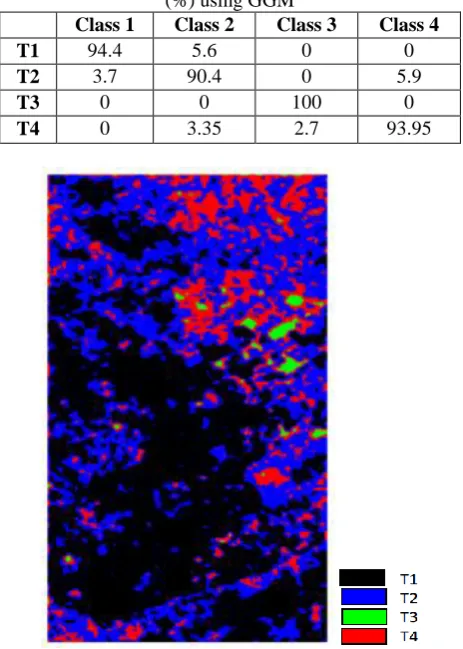
The best texture identification rate have been obtained for two wavelet decomposition levels and the scanning window 11x11. Then, the analysis by GGM, from the best classification results obtained, shows that the textures of this image have an identification rate more than 90% and less than 95%. The average rate of the good identification of the four textures is 94.69 %. Figure 28 shows the classified image by Generalized Gaussian Model.
Table VIII: Identification rate of radar textures in per cent (%) using GGM
Class 1 Class 2 Class 3 Class 4
T1 94.4 5.6 0 0
T2 3.7 90.4 0 5.9
T3 0 0 100 0
T4 0 3.35 2.7 93.95
Fig.28. Radar image classified by Generalized Gaussian Model
The figure 29 presents the comparison of the identification rate of texture radar image by the Gabor filter bank and the GGM. We can conclude, from the figure 29 that the classification method based on Gabor filter bank developed in this work gives the best results than the classification based on GMM.
Fig.29. Comparison of identification rate of radar texture image by Gabor filter bank and Generalized Gaussian
modeling
VI.
C
ONCLUSION ANDP
ERSPECTIVESIn this work, we have distinguished three fundamental aspects of the image research by contents: description, extraction and classification.
We have, in the first part, presented a texture characterization method based on Gabor filters and we have tested this frequential approach by the analysis of different texture types from de Brodatz data base. The results are interesting.
In the second part, the analysis of the textures of radar image allows us to generate the textural characteristics and to elaborate the filter banks for each texture. Textural signature vectors have been determined by the developed method. So, for each filter bank of a given texture, the characteristic vector is formed by two indexes: energy index designed by E and L1 norm.
The evaluation of the textural characterization has been operated by the supervised classification of radar image using mean square error between the signature vectors and the local characteristic vectors determined in the scanning windows. The classification results have been evaluated in terms of identification rate of the textures on the classified image.
The decomposition by the Gabor filters allows us to obtain the filtered images corresponding to each textural filter bank. Then, we have determined the optimal filter bank able to give the filtered images necessary for the determination of the textural characteristic vectors. These vectors have been used to classify the radar image and to evaluate the classification contribution in terms of textural identification. With this optimal filter bank, we have obtained the identification rate greater than 99%.
By comparing the classification results obtained by the Gabor filter bank that we have developed and the classification obtained by GGM, we have shown that our method based on Gabor filter bank give the best scores. The classification based on Gabor filter bank may be considered as a powerful and robust tool.
Copyright © 2014 IJECCE, All right reserved
R
EFERENCES[1] Cocquerez J.P., Philip S. : « Analyse d’images : filtrage et segmentation », Edition Dunod (1995).
[2] Borges G.A., Aldon M.-J. : « A split-and-merge segmentation algorithm for line extraction in 2D range images ». Pattern Recognition, Proceedings. 15th International Conference, spain 2000.
[3] Gagalowicz A. : « Vers un modèle de textures », Thèse de doctorat univ. Pierre et Marie Curie, Paris V, mai 1983. [4] Tuceryan M., Jain. A. K. : «Texture analysis ». Handbook of
Pattern recognition and computer vision , pages 235-276, 1993. [5] Sahbani H., Hamrouni K.: « Segmentation d’images textures par
transformée en ondelettes et classification C-moyenne floue », SETIT’2005, Sousse, Tunisie, 2005.
[6] Leblond I., Legris M., Basel S. :« Apport de la classification automatique d’images sonar pour le recalage à long terme ». Traitement du signal, 2008, Volume 25, N° 1-2 Numéro spécial, Pages 87-104.
[7] Dunn D., Higgins W.: « Optimal gabor filters for texture segmentation ». IEEE Trans on Image Processing, 4(7): 947-964, 1995.
[8] Marrakchi O., Chakroune H.: « Elaboration of texture filters for forest Aster image using Karhunen Loeve Transformation », GORS, Damascus-Syria, 7pages, 2008.
[9] Jebalia W. : «Développement des méthodes d’analyse de textures d’images de télédétection par TO et par MGG ; Elaboration de bancs de filtres des textures », Mastère, Institut National des Sciences Appliquées et Technologie de Tunis (INSAT), 2011. [10] VAUTROT P. : « Segmentation et classification d’images
texturées par filtrage spatio-fréquentiel : ondelettes splines et filtres de Gabor », PhD thesis, Université de Reims 1996. [11] Simona E., Petkov N., Kruizinga P.: « Comparison of texture
features based on gabor filters », IEEE Transactions on image processing, 11(10):1160-1067, 2002.
[12] GERMAIN C. « Analyse d’images et de textures orientées appliquée à la caractérisation de matériaux et à la télédétection ». Mémoire de D.E.A de physique, option Traitement du Signal et des Images,Université de Bordeaux1, Bordeaux, Juillet 2007. [13] Tuceryan M., Jain. A. K. : «Texture analysis ». Handbook of
Pattern recognition and computer vision , pages 235-276, 1993. [14] Kovalev V.A., Petrou M. : « Multidimensional cooccurrence
matrices for objet recognition and matching ». Graphical Models and Image Processing, 58(3): 187-197, 1996.
[15] HAFIANE A. : « Caractérisation de textures et segmentation pour la recherche d’images par le contenu ». Thèse de doctorat, université de Paris-Sud, 2005.
[16] Haralik R. M., Shanmugam K., Dinstein I. : « Textural features for image classification ». IEEE Transactions on Systems, Man and Cybernetics, 3 :610–621, Novembre 1973.
[17] Cross G.C., Jain A. K. : « Markov Random Field texture models ». IEEE Transactions on Pattern Analysis and Machine Intelligence, 5(1): 25-39, 1983.
[18] Dunn D., Higgins W., Weakley J. : « Texture segmentation using 2-D gabor elementary functions ». IEEE Trans. On Pattern Analysis and Machine Intelligence, 16(2): 130-1994.
[19] Turner M.R.: « Texture discrimination by gabor functions ». Biological Cybernetics, 55: 71-82, 1986.
[20] Jain A.K., Tuceryan M.: « Texture analysis », chapter 11 in the Handbook of pattern recognition and computer vision by C.H.Chen 1992.
[21] MARION1 A., VRAY1 D.. : « Filtrage spatiotemporel de séquences d’images ultrasonores pour l’estimation d’un champ dense de vitesses ». INSA-LYON, 2007.
[22] WELDON TP., HIGGINS WE. « Algorithm for designing multiple Gabor filters for segmenting multi-textured images », IEEE Inter. Conf. on Image Proc., 4-7, 1998.
[23] YANG F., LISHMAN, R.:« Land Cover Change Detection Using Gabor Filter Texture » Proceedings of the 3rd Inter. workshop on texture analysis and synthesis, pp. 78-83, 2003. [24] Bigün J., du Buf J.H.: « N-folded symmetries by complex
moments in Gabor space and their application to unsupervised texture segmentation », IEEE Trans. on Pattern Analysis and Machine Intelligence, Vol. 16, n°1, pp. 80-87, January 1994.
[25] Chen J., Sato Y., Tamura S.: « Orientation Space Filtering for Multiple Line Segmentation », Proc. of IEEE Conference on Computer Vision and Pattern Recognition, California, 1998. [26] Bruno E. : « De l’estimation locale à l’estimation globale de
mouvement dans les séquences d’images ». Thèse de doctorat, Université JOSEPH FOURIER, Laboratoire des Images et des Signaux de Grenoble, France, 2001.
[27] Michelet.F. :« Contribution a l’estimation d’orientations locales multiples dans les images numériques ». Thèse de doctorat Université Bordeaux1, 2006.
[28] Weldon T. P., Higgins W. E.: « Multiscale Rician approach to Gabor Filter design for texture segmentation », IEEE Int. Conf. on Image Processing, vol. II, (Austin, TX), 620{624, (13-16 Nov. 1994).
[29] Zhang J., Tan T.: « Brief review of invariant texture analysis methods », Pattern Recognition, vol. 35, pp. 735-747, 2002. [30] Randen T., Husoy J.H.: « Filtering for texture classification: A
comparative study », IEEE Trans. Pattern Analysis Match. Intell., vol.21, pp.291-310,1999.
[31] VIVEROS CANCINO O. : « Analyse du milieu urbain par une approche de fusion de données satellitaires optiques et radar », Thèse de doctorat univ. De Nice-Sophia Antipolis, juin 2003. [32] OUKIL A. : « Analyse variographique, modélisation et synthèse
de textures appliquées aux images numériques », Thèse de doctorat univ. De Sciences et de la Technologie, Houari Boumediene, Avril 2007.
[33] Majdoulayne H. : « Extraction de caractéristique de texture pour la classification d’images satellites », Thèse de doctorat Université de Toulouse, France, Décembre 2009.
[34] WELDON T. P., HIGGINS W. E.: « Designing Multiple Gabor Filters for Multi-Texture Image Segmentation ». Optical Engeneering 38(9) 1478-1489, septembre 1999.
[35] Laine A., Fan J.: « Texture classification by wavelet packet signatures ». IEEE Trans. Pattern Anal. Mach. Intell., 15(11) :1186–1191,1993.
[36] Randen T., Husoy J.H.: « Filtering for texture classification : A comparative study ». IEEE Trans. Pattern Anal. Machine Intell., 21(4) :291–310, April 1999.
[37] Luo B., Aujol J.-F., Gousseau Y., Ladjal S.: « Indexing of satellite images with different resolutions by wavelet features ». IEEE Trans.on IMage Processing, 17(8) :1465–1472, 2008. [38] Aujol J.F., Aubert G., Blanc-F L.: « Wavelet-based level set
evolution for classification of textured images », IEEE Trans. Image Processing, 12(12) :1634–1641, 2003.
[39] O. Marrakchi, J. Mbainaibeye and W. Jebalia, «Wavelet-Based Remote Sensing Heterogeneous Texture Signatures Using Generalized Gaussian Density Model», International Review on Computers and Software (IRECOS), ISSN 1828-6003, Vol.7, No.2, pp.538-545, Praise worthy prize, March 2012.
A
UTHOR’
SP
ROFILEDr. Mbainaibeye Jérôme
Copyright © 2014 IJECCE, All right reserved