University of New Orleans University of New Orleans
ScholarWorks@UNO
ScholarWorks@UNO
University of New Orleans Theses and
Dissertations Dissertations and Theses
Spring 5-13-2016
Automated Sea State Classification from Parameterization of
Automated Sea State Classification from Parameterization of
Survey Observations and Wave-Generated Displacement Data
Survey Observations and Wave-Generated Displacement Data
Jason A. Teichman
University of New Orleans, New Orleans, [email protected]
Follow this and additional works at: https://scholarworks.uno.edu/td
Part of the Applied Statistics Commons, Other Physics Commons, and the Statistical Models Commons
Recommended Citation Recommended Citation
Teichman, Jason A., "Automated Sea State Classification from Parameterization of Survey Observations and Wave-Generated Displacement Data" (2016). University of New Orleans Theses and Dissertations. 2199.
https://scholarworks.uno.edu/td/2199
This Thesis is protected by copyright and/or related rights. It has been brought to you by ScholarWorks@UNO with permission from the rights-holder(s). You are free to use this Thesis in any way that is permitted by the copyright and related rights legislation that applies to your use. For other uses you need to obtain permission from the rights-holder(s) directly, unless additional rights are indicated by a Creative Commons license in the record and/or on the work itself.
Automated Sea State Classification from Parameterization of Survey Observations and Wave-Generated Displacement Data
A Thesis
Submitted to the Graduate Faculty of the University of New Orleans in partial fulfillment of the requirements for the degree of
Master of Science in
Applied Physics
by
Jason A. Teichman
B.S. Ferris State University, 2002
ii
Approved for public release; distribution is unlimited.
iii
ACKNOWLEDGEMENTS
There are a great number of people who have contributed to the realization of this thesis.
My greatest thanks go out to Gus Michel, Lisa Pflug, Garry Owen, David Bates, and Wes
Hillstrom. Your input and guidance kept me on-track and endlessly thinking. I would like to
express my appreciation to Susan Sebastian, Clay Whittaker, and Theresa Anoskey for taking the
time to walk me through many of the initial steps needed to gather my data. Thank you to the
Naval Oceanographic Office, Mr. Randall Hill, and Dr. Michael Wild for graciously granting me
the funding and time to work through this thesis, and to all of my colleagues who filled the void
as I remained focused. Endless and ongoing thanks to my UNO thesis advisors Dr. Juliette Ioup
and Dr. Stanley Chin-Bing for the years of education and patience. Lastly, warmest regards to
iv
TABLE OF CONTENTS
LIST OF FIGURES ... vi
LIST OF TABLES ... ix
ABSTRACT ... xii
CHAPTER 1 - INTRODUCTION ... 1
1.A. Sea State ... 1
1.B. Limitations ... 4
1.B.1. Observations ... 4
1.B.2. Operations and Safety ... 5
1.C. Prior Research of Sea State Automation ... 6
1.D. Proposed Research ... 7
CHAPTER 2 - SURVEY DATA AND OBSERVATIONS ... 9
2.A. Data Collection ... 9
2.B. Extraction and Quality Control... 11
2.C. Data Analysis ... 13
2.C.1. Selected Data ... 13
2.C.2. Seasonal and Visibility Information ... 16
2.C.3. Wind Scale Comparisons ... 18
CHAPTER 3 – METHODS AND RESULTS ... 21
3.A. Considerations ... 21
3.B. Displacement ... 22
3.B.1. Absolute Displacement (AD) ... 22
3.B.2. Mean Absolute Displacements ... 23
3.B.3. Scaling Factors ... 24
3.B.4. Power Spectral Density ... 28
3.B.5. Outliers ... 32
3.C. Distribution Fitting ... 33
3.C.1. Distributions ... 33
3.C.2. Tolerance and Confidence Intervals ... 39
v
3.E. Model Testing and Results ... 45
3.E.1. Trial A Plots ... 48
3.E.2. Trial A Analysis ... 61
3.E.3. Trial B ... 66
3.E.4. Trial B Analysis ... 75
3.F. Additional Analysis... 77
CHAPTER 5 – FURTHER RESEARCH ... 80
REFERENCES ... 81
APPENDICES ... 83
A. Matlab Pseudo Code and Descriptions ... 83
B. Data Statistics ... 84
C. Distribution Parameters ... 92
D. Tolerance Interval Tables ... 94
E. Confidence Interval Tables ... 106
F. Model Boundaries (only upper limits are shown) ... 118
G. Trail A Matching Tables ... 121
H. Trial B Matching Tables... 126
vi
LIST OF FIGURES
Figure 1. Sea State Frequencies ... 15
Figure 2. Spring Surveys... 17
Figure 3. Summer Surveys ... 17
Figure 4. Fall Surveys ... 17
Figure 5. Winter Surveys ... 17
Figure 6. Beaufort SS Conversion vs. Observed SS ... 19
Figure 7. Operational SS vs. Observed SS ... 19
Figure 8. AMTAD Correlation ... 28
Figure 9. RMSTAD Correlation ... 28
Figure 10. Event #300 Roll Spectrum... 30
Figure 11. Event #303 Roll Spectrum... 30
Figure 12. Power Spectrum of Roll ... 31
Figure 13. Power Spectrum of Pitch ... 31
Figure 14. Power Spectrum of Heave ... 31
Figure 15. Power Spectrum of TAD ... 31
Figure 16a. Gaussian Probability Plot of AMTAD ... 34
Figure 16b. Gaussian Probability Plot of RMSTAD ... 34
Figure 17a. Weibull Probability Plot of AMTAD ... 35
Figure 17b. Weibull Probability Plot of RMSTAD ... 35
Figure 18a. Rayleigh Probability Plot of AMTAD ... 36
Figure 18b. Rayleigh Probability Plot of RMSTAD ... 36
Figure 19a. Lognormal Probability Plot of AMTAD ... 37
Figure 19b. Lognormal Probability Plot of RMSTAD ... 37
Figure 20. Sea State 1 AMTAD and Associated Distributions ... 38
Figure 21. Sea State 2 AMTAD and Associated Distributions ... 38
Figure 22. Sea State 3 AMTAD and Associated Distributions ... 39
Figure 23a. Trial A – Sea State 0 – Event 196 ... 48
Figure 23b. Trial A – Sea State 0 – Event 218 ... 48
Figure 23c. Trial A – Sea State 0 – Event 226 ... 49
Figure 23d. Trial A – Sea State 0 – Event 275 ... 49
Figure 24a. Trial A – Sea State 1 – Event 038 ... 50
Figure 24b. Trial A – Sea State 1 – Event 156 ... 50
vii
Figure 24d. Trial A – Sea State 1 – Event 291 ... 51
Figure 25a. Trial A – Sea State 2 – Event 023 ... 52
Figure 25b. Trial A – Sea State 2 – Event 078 ... 52
Figure 25c. Trial A – Sea State 2 – Event 289 ... 53
Figure 25d. Trial A – Sea State 2 – Event 372 ... 53
Figure 26a. Trial A – Sea State 3 – Event 080 ... 54
Figure 26b. Trial A – Sea State 3 – Event 159 ... 54
Figure 26c. Trial A – Sea State 3 – Event 332 ... 55
Figure 26d. Trial A – Sea State 3 – Event 362 ... 55
Figure 27a. Trial A – Sea State 4 – Event 094 ... 56
Figure 27b. Trial A – Sea State 4 – Event 208 ... 56
Figure 27c. Trial A – Sea State 4 – Event 229 ... 57
Figure 27d. Trial A – Sea State 4 – Event 356 ... 57
Figure 28a. Trial A – Sea State 5 – Event 065 ... 58
Figure 28b. Trial A – Sea State 5 – Event 238 ... 58
Figure 28c. Trial A – Sea State 5 – Event 345 ... 59
Figure 28d. Trial A – Sea State 5 – Event 363 ... 59
Figure 29a. Trial A – Sea State 6 – Event 236 ... 60
Figure 29b. Trial A – Sea State 6 – Event 237 ... 60
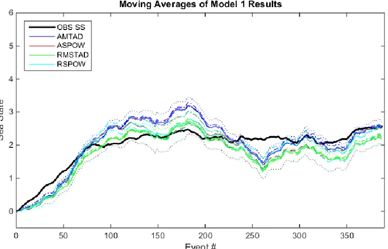
Figure 30. Trial A – Model 1 Results ... 62
Figure 31. Trial A – Model 2 Results ... 62
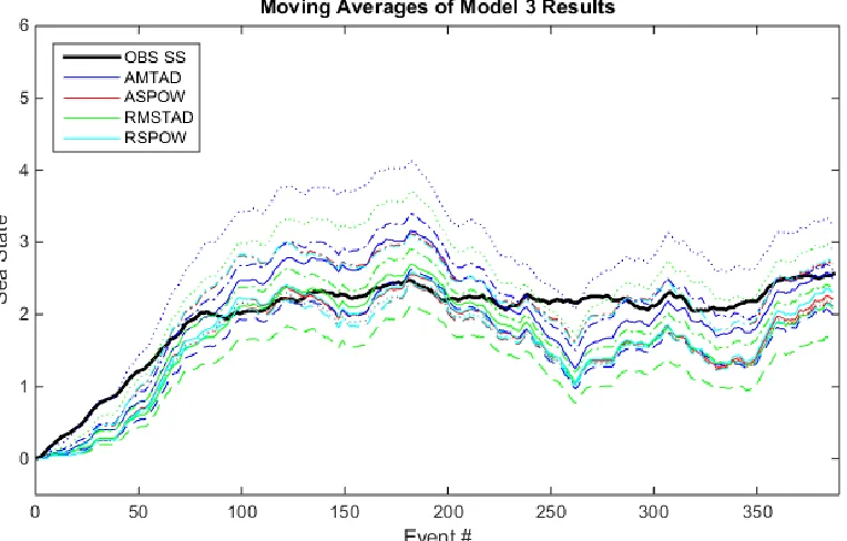
Figure 32. Trial A – Model 3 Results ... 63
Figure 33. Trial A – Model 4 Results ... 63
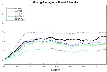
Figure 34. Trial A – Model 5 Results ... 64
Figure 35. Trial B – Sea State 0 – Event 395... 66
Figure 36a. Trial B – Sea State 1 – Event 388 ... 67
Figure 36b. Trial B – Sea State 1 – Event 389... 67
Figure 36c. Trial B – Sea State 1 – Event 392 ... 68
Figure 37a. Trial B – Sea State 2 – Event 393 ... 69
Figure 37b. Trial B – Sea State 2 – Event 394... 69
Figure 37c. Trial B – Sea State 2 – Event 396 ... 70
Figure 37d. Trial B – Sea State 2 – Event 407... 70
Figure 38a. Trial B – Sea State 3 – Event 391 ... 71
viii
Figure 38c. Trial B – Sea State 3 – Event 404 ... 72
Figure 38d. Trial B – Sea State 3 – Event 406... 72
Figure 39a. Trial B – Sea State 4 – Event 409 ... 73
Figure 39b. Trial B – Sea State 4 – Event 410... 73
Figure 40. Trial B – Sea State 5 – Event 408... 74
ix
LIST OF TABLES
Table 1. WMO Sea State Scale ... 1
Table 2. Beaufort Wind Scale ... 2
Table 3. Survey Operations Sea State Scale ... 3
Table 4. Pre-Selected Survey Events by Sea State ... 9
Table 5. Minimum Sample Sizes ... 12
Table 6. Selected Survey Events by Sea State ... 14
Table 7. Selected Survey Data ... 14
Table 8. Event Count by Ship Platform ... 15
Table 9. Observational Visibility ... 16
Table 10. Pearson Correlation Coefficients of Pre-Scaled Displacement to Sea State ... 24
Table 11. Scaling Factors ... 26
Table 12. Pearson Correlation Coefficients of Pre-Scaled vs. Scaled Data... 27
Table 13. Potential Outliers ... 32
Table 14. Model 5 Boundaries for Non-logarithmic AMTAD Data ... 44
Table 15. Randomly Selected Events for Trial A ... 46
Table 16. Selected Survey Event Count by Sea State ... 46
Table 17. Randomly Selected Events for Trial B ... 47
Table 18. Trial A – Model Sea State Matching ... 61
Table 19. Trial A – Total Model Mean Sea State Margin Matching ... 65
Table 20. Trial B – Model Sea State Matching ... 75
Table 21. Trial B – Total Model Mean Sea State Margin Matching ... 76
Table 22. Visibility Margin Matching ... 77
Table B1. Pre-Scaled MAD Data Statistics ... 84
Table B2. Pre-Scaled MTAD Data Statistics ... 85
Table B3. Scaling Factors ... 86
Table B4. Scaled MAD Data Statistics ... 87
Table B5. Scaled MTAD Data Statistics (Outliers Included) ... 88
Table B6. Scaled MTAD Data Statistics (Outliers Removed) ... 89
Table B7. Scaled SPOW Data Statistics (Outliers Included) ... 90
Table B8. Scaled SPOW Data Statistics (Outliers Removed) ... 91
Table C1. Distribution Parameters (Outliers Included) ... 92
Table C2. Distribution Parameters (Outliers Removed) ... 93
x
Table D2. 90% and 95% AMTAD/ASPOW Tolerance Intervals (Outliers Included) ... 95
Table D3. 99% AMTAD/ASPOW Tolerance Intervals (Outliers Included) ... 96
Table D4. 70% and 80% RMSTAD/RSPOW Tolerance Intervals (Outliers Included) ... 97
Table D5. 90% and 95% RMSTAD/RSPOW Tolerance Intervals (Outliers Included) ... 98
Table D6. 99% RMSTAD/RSPOW Tolerance Intervals (Outliers Included) ... 99
Table D7. 70% and 80% AMTAD/ASPOW Tolerance Intervals (Outliers Removed) ... 100
Table D8. 90% and 95% AMTAD/ASPOW Tolerance Intervals (Outliers Removed) ... 101
Table D9. 99% AMTAD/ASPOW Tolerance Intervals (Outliers Removed) ... 102
Table D10. 70% and 80% RMSTAD/RSPOW Tolerance Intervals (Outliers Removed) ... 103
Table D11. 90% and 95% RMSTAD/RSPOW Tolerance Intervals (Outliers Removed) ... 104
Table D12. 99% RMSTAD/RSPOW Tolerance Intervals (Outliers Removed) ... 105
Table E1. 70% and 80% AMTAD/ASPOW Confidence Intervals (Outliers Included) ... 106
Table E2. 90% and 95% AMTAD/ASPOW Confidence Intervals (Outliers Included) ... 107
Table E3. 99% AMTAD/ASPOW Confidence Intervals (Outliers Included) ... 108
Table E4. 70% and 80% RMSTAD/RSPOW Confidence Intervals (Outliers Included) ... 109
Table E5. 90% and 95% RMSTAD/RSPOW Confidence Intervals (Outliers Included) ... 110
Table E6. 99% RMSTAD/RSPOW Confidence Intervals (Outliers Included) ... 111
Table E7. 70% and 80% AMTAD/ASPOW Confidence Intervals (Outliers Removed) ... 112
Table E8. 90% and 95% AMTAD/ASPOW Confidence Intervals (Outliers Removed) ... 113
Table E9. 99% AMTAD/ASPOW Confidence Intervals (Outliers Removed)... 114
Table E10. 70% and 80% RMSTAD/RSPOW Confidence Intervals (Outliers Removed) ... 115
Table E11. 90% and 95% RMSTAD/RSPOW Confidence Intervals (Outliers Removed) ... 116
Table E12. 99% RMSTAD/RSPOW Confidence Intervals (Outliers Removed) ... 117
Table F1. Model 1 Sea State Boundaries ... 118
Table F2. Model 2 Sea State Boundaries ... 118
Table F3. Model 3 Sea State Boundaries ... 119
Table F4. Model 4 Sea State Boundaries ... 119
Table F5. Model 5 Sea State Boundaries ... 120
Table G1a. Model Run A - Model 1 – Model Sea State Matching ... 121
Table G1b. Model Run A - Model 1 – Model Mean Sea State Margin Matching ... 121
Table G2a. Model Run A - Model 2 – Model Sea State Matching ... 122
Table G2b. Model Run A - Model 2 – Model Mean Sea State Margin Matching ... 122
Table G3a. Model Run A - Model 3 – Model Sea State Matching ... 123
xi
Table G4a. Model Run A - Model 4 – Model Sea State Matching ... 124
Table G4b. Model Run A - Model 4 – Model Mean Sea State Margin Matching ... 124
Table G5a. Model Run A - Model 5 – Model Sea State Matching ... 125
Table G5b. Model Run A - Model 5 – Model Mean Sea State Margin Matching ... 125
Table H1a. Model Run B - Model 1 – Model Sea State Matching ... 126
Table H1b. Model Run B - Model 1 – Model Mean Sea State Margin Matching ... 126
Table H2a. Model Run B - Model 2 – Model Sea State Matching ... 127
Table H2b. Model Run B - Model 2 – Model Mean Sea State Margin Matching ... 127
Table H3a. Model Run B - Model 3 – Model Sea State Matching ... 128
Table H3b. Model Run B - Model 3 – Model Mean Sea State Margin Matching ... 128
Table H4a. Model Run B - Model 4 – Model Sea State Matching ... 129
Table H4b. Model Run B - Model 4 – Model Mean Sea State Margin Matching ... 129
Table H5a. Model Run B - Model 5 – Model Sea State Matching ... 130
xii
ABSTRACT
Sea state is a subjective quantity whose accuracy depends on an observer’s ability to
translate local wind waves into numerical scales. It provides an analytical tool for estimating the
impact of the sea on data quality and operational safety. Tasks dependent on the characteristics
of local sea surface conditions often require accurate and immediate assessment. An attempt to
automate sea state classification using eleven years of ship motion and sea state observation data
is made using parametric modeling of distribution-based confidence and tolerance intervals and a
probabilistic model using sea state frequencies. Models utilizing distribution intervals are not
able to exactly convert ship motion data into various sea states scales with significant accuracy.
Model averages compared to sea state tolerances do provide improved statistical accuracy but the
results are limited to trend assessment. The probabilistic model provides better prediction
potential than interval-based models, but is spatially and temporally dependent.
1
CHAPTER 1 - INTRODUCTION
1.A. Sea State
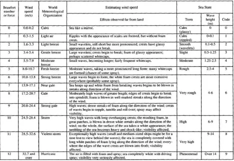
The modern WMO (World Meteorological Organization) Sea State Scale in Table 1
(WOCE, 2002) describes the properties of locally driven, open-ocean wind waves. The code
ranges from 0 (the calmest of conditions; the sea has a mirror-like appearance) to 9 (the worst
conditions possible). The appearance of wind waves is predominantly generated by winds, the
duration of the wind at speed, and the duration and size of the wind fetch; factors such as strong
currents, precipitation, tides, and ice formations can also affect the developed sea state (White
and Hanson, 2000). Swells are generally considered to be separate from wind waves, but the
angle of the wind direction to the swell direction can significantly affect the agitation of local
waves.
Table 1. WMO Sea State Scale
Code Figure Descriptive terms Wind-Wave Height (meters)
0 Calm (glassy) 0
1 Calm (rippled) 0 - 0.1
2 Smooth (wavelets) 0.1 - 0.5
3 Slight 0.5 - 1.25
4 Moderate 1.25 - 2.5
5 Rough 2.5 - 4
6 Very rough 4 - 6
7 High 6 - 9
8 Very high 9 - 14
9 Phenomenal Over 14
Determination of sea state has traditionally been an in-situ process that requires
subjective measurement, limited by the skill level of the observer and the observational
2
descriptive terms of the table are used as the primary guidance for classifying the seas; the
wind-wave height becomes a secondary validation to the observer’s sea state assessment.
Wind-wave conditions are often described and compared with the ubiquitous Beaufort
Wind Scale which was developed and accepted into practice in the early 1800s. This scale is
used in the maritime industry, including the organization responsible for the operation and
maintenance of the survey ships that provided the data in this study. The Beaufort Wind Scale
with corresponding WMO Sea State Codes is shown in Table 2 (Bowditch, 1995).
3
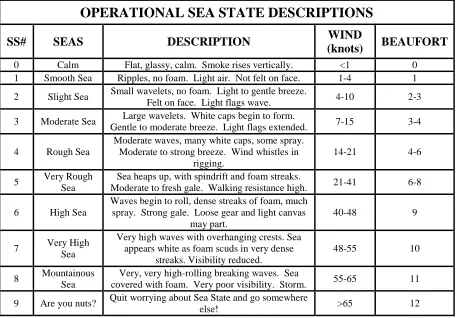
The sea state codes used by the scientific teams aboard the survey vessels that provided
the data in this study are a modified form of the WMO and Beaufort tables. This table is adjusted
to represent specific mission requirements and is dependent primarily on wind speed and a
description of the local sea conditions. Table 3 details the wind and sea surface conditions
required to select operationally sound conditions for the surveys in this study (Velazquez-Aviles
et al., 1999-2014). This sea state scale will be referred to as the Operational Scale. It is expected
that this table has been followed to some degree of accuracy by all observers since 2004.
Table 3. Survey Operations Sea State Scale
OPERATIONAL SEA STATE DESCRIPTIONS
SS# SEAS DESCRIPTION WIND
(knots) BEAUFORT 0 Calm Flat, glassy, calm. Smoke rises vertically. <1 0 1 Smooth Sea Ripples, no foam. Light air. Not felt on face. 1-4 1
2 Slight Sea Small wavelets, no foam. Light to gentle breeze.
Felt on face. Light flags wave. 4-10 2-3
3 Moderate Sea Large wavelets. White caps begin to form.
Gentle to moderate breeze. Light flags extended. 7-15 3-4
4 Rough Sea
Moderate waves, many white caps, some spray. Moderate to strong breeze. Wind whistles in
rigging.
14-21 4-6
5 Very Rough Sea
Sea heaps up, with spindrift and foam streaks.
Moderate to fresh gale. Walking resistance high. 21-41 6-8
6 High Sea
Waves begin to roll, dense streaks of foam, much spray. Strong gale. Loose gear and light canvas
may part.
40-48 9
7 Very High Sea
Very high waves with overhanging crests. Sea appears white as foam scuds in very dense
streaks. Visibility reduced.
48-55 10
8 Mountainous Sea
Very, very high-rolling breaking waves. Sea
covered with foam. Very poor visibility. Storm. 55-65 11
9 Are you nuts? Quit worrying about Sea State and go somewhere
4
The Douglas Sea State Scale developed in the 1920s converts wave and swell heights into
similar numerical codes, but given the subjective nature of these measurements, this scale is not
included.
1.B. Limitations
1.B.1. Observations
Sea state measurements that are founded on ocean wave characteristics are limited by the
ability of the observer to discern wave characteristics and categorize the observations into an
appropriate scaling. The observer may have a limited skill set or may be impeded from making a
sound observation by weather or visibility conditions that prevent an accurate assessment. This is
particularly true at night, when determining a wind-wave sea state is almost impossible. In
addition, mariners and scientists are given multiple scales to consider, and it is possible that
scales used in one event are not the same scales used in another event. Although the confusion
and subjectivity of observations have still produced many successful missions, there is a
noticeable loss or corruption of data due to operations conducted in conditions that were
misdiagnosed or rapidly changing.
The survey events in this study require the use of sea state as a predictor of data quality
and operational safety. Some of the operations were conducted at night; sea states in these cases
5
1.B.2. Operations and Safety
Reliable estimation of sea state is essential to decision support systems for effective
oceanographic operations. Oceanographic operations that require calm conditions to perform
adequately are dependent on the state of the sea. This study was developed from a need intrinsic
to acoustic operations. In the survey events from which this study is derived, operational safety
and noise are leading concerns and an accurate sea state assessment provides operations leaders
with a more complete picture of the state of the sea. The subjective nature of the assessment has
created a climate of contention in the community of operators. This study will attempt to
alleviate the subjectivity and provide a more objectively quantifiable assessment base.
Every surface mission has sea-state limitations. In most cases, the limiting sea state is 4
or 5 (NAVOCEANO, 1999; NAVOCEANO Personnel, 2015). At sea state 4, concern for
operational safety becomes significant. Sea states higher than 4 can severely impact operational
safety. Higher sea states also render certain oceanographic missions ineffective. For example, sonobuoy radio frequency (RF) dropout created by a “washover” of the signal output equipment
often occurs with seas that are above sea state 5 (NAVOCEANO, 1999).
Ambient noise levels increase with sea state, especially in the frequency range between
300 and 5000 Hz (NAVOCEANO, 1999). For each increase by 1 in the sea state code, ambient
noise levels increase by approximately 6 dB (NAVOCEANO, 1999) and as much as 10 dB
depending on the frequency and depth (Waite, 2005). In survey operations where good signal
6
1.C. Prior Research of Sea State Automation
The connection of wave characteristics to the sea state has been studied throughout most
of the second half of the 20th century. Attempts to mitigate the problem of observational
subjectivity have been a prominent subspace of this research. Although there have been many
studies conducted by civilian and governmental organizations, only a few noteworthy
publications are provided.
In the early 1950s, Diede and Thieme [5] conducted a general survey of the studies and
instruments being developed for measurement of wind conditions and wave heights, lengths, and
frequencies. They produced a summarization of the progress made in aircraft measurement
devices and the use of optics to determine wave characteristics. They noted that at the time of the
survey, only the U.S., England, Germany, and France were conducting studies in this area. Their
conclusions made note of the optimism of the future for the research being conducted.
A preliminary study published by Clayton, Ivey, and Teegardin in 1954 [3] was
conducted to develop a sea state meter using bare and dielectric-coated wires in conjunction with
a slope-measuring unit created for the experiment. It was intended to produce height and slope
data of ocean waves in an attempt to statistically determine sea state. Their experimental cycle
rates were too low to produce the results they desired, but as of the time of the publication, they
had determined a rate that showed promise.
Black and Adams [1] utilized vertically pointing aircraft photos to determine surface
winds in an attempt to record Beaufort wind force values. This was done to assist in the training
7
In the fall of 1989, scientists at the Naval Underwater Systems Center conducted
experiments using the newly patented Submarine-Deployed Sea State Sensor (SUDSS)
(Shonting et al., 1989). They were able to show the device had the ability to take a wide variety
of sea surface measurements with varying degrees of accuracy. Other methods were eventually
developed by the submarine community, and at present, the SUDSS is not being used
operationally (NAVOCEANO Personnel, 2015).
Work published in 2000 by White and Hanson [29] at Johns Hopkins University utilized
directional wave spectra and wind velocity data obtained from National Data Buoy Center
(NDBC) weather buoys to create an effective wind speed that could then be translated into a
Beaufort force and corresponding sea state codes. Their tests concluded that calculated sea states
reasonably coincided with visually observed sea states.
As of the development of this thesis, no known attempts to connect sea state observations
with vessel displacement measurements have been published.
1.D. Proposed Research
The intent of this study is to connect sea state observations with associated in-situ
wave-riding characteristics of a naval survey vessel in an attempt to find a meaningful, deterministic
model that can numerically assess the state of the sea with a significant degree of accuracy. It
should be sufficient to utilize statistical methods to develop a parameterization of sea-state
specific data that can be used to determine if information produced by displacement
measurements fall within parameters of a given sea state. A distribution fitting method using
8
these effects) will provide the limits that will be used in various modeling schemes. A variety of
probability distribution types will be used. If a specific distribution provides a significantly more
accurate assessment, the limits developed will drive the applied routines for this study. If there is
a substantially uniform return for the distributions used, a more comprehensive use of the
parameters may be examined.
Although wind contributes greatly to the state of local seas, its inherent variability in both
speed and direction limit its use as an effective measurement for the purposes of this study.
Average wind speeds are used to determine Beaufort and operational sea state codes in an
attempt to determine if model results can additionally predict the measurements from these
scales. It is expected that further development of this research will eventually include wind
measurements in some form.
It should be noted that if a relationship between sea state and ship displacement exists
and a deterministic method can be developed for predicting the state of the sea, the data must be
managed in real time using shipboard acquisition and processing systems. Any model developed
must contain algorithms that do not place unrealistic computational demands on the shipboard
9
CHAPTER 2 - SURVEY DATA AND OBSERVATIONS
2.A. Data Collection
The data sets used for this study were collected from naval oceanographic surveys from
2004 to 2014. A total of 19 surveys were conducted in similar geographical locations, each
survey consisting of between 7 and 36 individual survey events. Each event ranged from
approximately 15 minutes to 3 hours. In earlier surveys, more than one event was conducted
daily; later surveys are generally limited to one survey event per day. Collectively, there were a
total of 410 separate survey events.
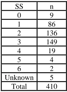
Table 4 details a parsing of the total number of recorded events by sea state. The
unknown values represent events that had no sea state observation record.
Table 4. Pre-Selected Survey Event Count by Sea State
The data were produced by crews and measurement systems aboard three naval survey
vessels. Each ship was of the same construction class and sufficiently similar to be considered
the same platform type for the purposes of measurement standardizations.
SS n
0 9
1 86
2 136
3 149
4 19
5 4
6 2
Unknown 5
10
During each event, a shipboard inertial navigation system provided in-situ dynamic data,
and an anemometer-based system measured both true and apparent wind speeds. The ship’s
Inertial Measurement Unit (IMU) utilized angular accelerometers to measure gravitation-based
angular displacements (roll, pitch, and yaw), and linear accelerometers to measure
non-gravitational accelerations that translate to linear motion displacements (heave, surge, and sway)
(Eschbach et al., 1990; King, 1998). A calibrated gyroscopic element in the IMU is utilized to
maintain an absolute plane of reference. The ship’s axes were periodically updated to maintain a
zeroed axis plane of reference (NAVOCEANO Personnel, 2015); the standard practice of ship
axes calibration for the purpose of sensor performance and accuracy is expected and was
confirmed by header data used to display each offset and its calibration. All dynamic and
environmental data collected by the sensors were then chronologically recorded in an onboard
system that parses and archives the data in the highest resolutions available.
A sea state observation based on the scaling in Table 3 was made at some time during the
event (the exact time is never recorded). It was expected that the observer used the scale in Table
3, but observational tempo or limitations sometimes relegated the task of sea assessment to the ship’s crew who exclusively used the Beaufort scaling in Table 2. In some cases the sea state
changed during the event; in these instances, the higher sea states were used for this analysis.
This was done to reflect the greater variability in the ship motion due to the increased sea
conditions and represents a conservative estimate that leans in the direction of operational safety.
Since surveys required operationally effective seas, only measurements of sea state 0 to sea state
11
A shipboard anemometer was used to record the wind speed and direction. Processing
software produced both apparent and true wind speeds and directions. For the purpose of this
study, only true wind speeds are considered.
2.B. Extraction and Quality Control
The raw, time-series displacement and wind data from organizational archives were
downloaded using LINUX/UNIX command-line functions and parsed by survey and Julian date.
To achieve the largest relevant sampling possible only events with periods greater than or
equal to an hour were included; all other samples were rejected. Most samples were in excess of
an hour but generally less than 2.5 hours. The only exception to this rejection criterion was a sea
state 6 event with less than an hour of data. This event was not rejected in an attempt to provide
sea state 6 data; there are only two sea state 6 events.
Events that were missing key information such as a sea state observation were rejected.
Missing wind data was not considered a rejection criterion; wind is not used to provide limiting
parameters in this study. Additionally, if the ship’s course was not reasonably consistent, the
event was rejected. Course changes can cause significant roll or pitch to occur which could
contaminate the data for the purposes of this study.
A total of 23 survey events were rejected.
Since the purpose of this study is to utilize statistical arguments to justify the parameters
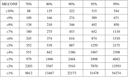
needed to develop a sea state model, sample sizes in Table 4 are questionable. For example,
given a standard deviation of 𝜎 ≈ 0.90521 determined through preliminary testing, with a
12 𝑀𝐸 = 𝑧∗ 𝜎
√𝑛
where 𝑧∗ = 1.037, 1.282, 1.645, 1.960 and 2.576 for confidence levels of 70%, 80%, 90%,
95%, and 99%, respectively, requires minimum sample sizes as detailed in Table 5 for margins
of error ranging from ±1% to ±10%.
Table 5. Minimum Sample Sizes
ME\CONF 70% 80% 90% 95% 99%
±10% 88 135 222 315 544
±9% 109 166 274 389 671
±8% 138 210 346 492 850
±7% 180 275 453 642 1110
±6% 245 374 616 874 1510
±5% 352 539 887 1259 2175
±4% 551 842 1386 1967 3398
±3% 979 1496 2464 3498 6042
±2% 2203 3367 5543 7870 13593
±1% 8812 13467 22173 31478 54374
This criterion suggests that only parameters and results using sea state data from sea
states 2 and 3 can be considered statistically significant. Specifically, the sample sizes in Table 5
allow a minimum margin of error of 9% for a 70% confidence level for sea state 2, and a
minimum margin of error of 8% for a 70% confidence level or 10% for an 80% confidence. Due
13
70% for most of the data. Discussions relevant to all other sea states will be speculation based on
trends.
2.C. Data Analysis
The following sections discuss the particular facets of the extracted data. Section 2.C.1.
covers the extraction counts and partitions as well as a brief discussion of the sea state
frequencies. An overview of the seasonal and diurnal observations is covered in section 2.C.2. A
comparison of observed sea states to wind-generated Beaufort and Operational scales is
accomplished in section 2.C.3. This analysis is conducted to provide comprehensive statistics of
the selected data sets, and to provide conditions and validations for further analysis.
2.C.1. Selected Data
A total of 387 events were selected for inclusion in this study and assigned a number
from 001 to 387. Table 6 is the selected event count by sea state. Table 7 details each survey and
its associated Julian date range, number of individual selected events, and sampling resolution.
14
Table 6. Selected Survey Event Count by Sea State
Table 7. Selected Survey Data
It should be noted that Surveys 5 and 6 do not have any associated wind data.
SS n
0 9
1 81
2 129
3 146
4 16
5 4
6 2
Total 387
Survey # JD Range Event # Res (sec)
1 144 – 159 21 0.52
2 170 – 191 32 0.52
3 037 – 061 21 0.52
4 073 – 095 25 0.52
5 169 – 192 23 1.04
6 202 – 227 20 1.04
7 231 – 251 23 0.52
8 264 – 284 17 0.52
9 240 – 254 23 0.50
10 264 – 284 12 0.50
11 058 – 083 30 0.20
12 135 – 158 33 0.20
13 173 – 196 18 0.20
14 180 – 199 24 0.10
15 217 – 233 22 0.10
16 292 – 304 12 0.10
17 326 – 336 7 0.10
18 282 – 310 17 0.10
19 320 – 332 7 0.10
15
Table 8. Event Count by Ship Platform
The boxplot in Figure 1 displays the event frequency and associated probability of the
occurrence of each sea state. Given the wide wind variety available in the Operational scaling
codes, there is a greater likelihood of sea states existing from 1 to 3. Operationally, sea state 3
conveys the greatest sea condition variability and the larger number of sea state 3 observations
suggest validity to this claim.
Figure 1. Sea State Frequencies Ship # of Events
#
1 298
2 65
16
A similar distribution of sea state frequencies is available in a technical report by
Shonting, Hebda, McCarthy, and Chaves (1989).
2.C.2. Seasonal and Visibility Information
Surveys were conducted in both temperate and equatorial climates, under all possible
conditions of visibility. The majority of surveys were done in the lower latitudes making the
impact of seasonal data less significant. Although not specifically beneficial to this study,
seasonal information provides an environmental backdrop for further research. Visibility
conditions have a greater influence on the assessment of the state of the sea, and subsequently,
survey events are parsed by light conditions to enhance environmental intelligence as it pertains
to this study.
A meteorological season standard (NOAA, 2013) is used to partition survey events, such
that for non-leap years, the Julian date ranges are: spring (60-151), summer (152-243), fall
(244-334), and winter (1-59, 335-365), and for leap years: spring (61-152), summer (153-244), fall
(245-335), and winter (1-60, 336-366). Given this scheme, there were a total of 85 spring
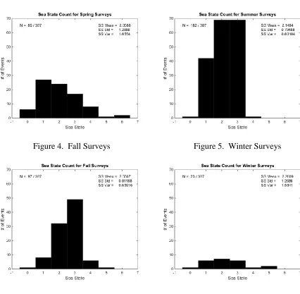
surveys, 182 summer surveys, 97 fall surveys, and 23 winter surveys. Figures 2-5 are histograms
17
Figure 2. Spring Surveys Figure 3. Summer Surveys
Figure 4. Fall Surveys Figure 5. Winter Surveys
Visibility has a substantial impact on the assessment of the sea. Given the potential for
inaccurate sea state assessments due to nighttime (poor light) observations, it is important to note
the number of survey events conducted in good and poor light conditions. If it is expected that
limited visibility begins due to nightfall, approximately 21:00 (military time) on average, which
prevails until approximately 05:00, then observations that are made within this period will be
considered limited by poor lighting. The light conditions and associated counts for each of the
18
Table 9. Observational Visibility Counts
2.C.3. Wind Scale Comparisons
The observed sea states in events that have associated wind data (Surveys 1-4, 7-19) were
compared to Beaufort and Operational sea states using the mean of the true wind speed for the
duration of the event. Although the wind speed average may not have coincided directly with the
wind speed at the time of the observation, the mean was sufficient to show the trend of the wind
in the event locale.
Survey # Good
Light %
Poor
Light %
1 11 52.4 10 47.6
2 25 78.1 7 21.9
3 15 71.4 6 28.6
4 14 56.0 11 44.0
5 17 73.9 6 26.1
6 12 60.0 8 40.0
7 14 60.9 9 39.1
8 12 70.6 5 29.4
9 15 65.2 8 34.8
10 10 83.3 2 16.7
11 25 83.3 5 16.7
12 26 78.8 7 21.2
13 12 66.7 6 33.3
14 12 50.0 12 50.0
15 17 77.3 5 22.7
16 9 75.0 3 25.0
17 5 71.4 2 28.5
18 15 88.2 2 11.8
19 6 85.7 1 14.3
19
Average winds speeds for each event were converted to the Beaufort and Operational sea
state codes on Tables 2 and 3, respectively. The sea states were then compared for each event
and a count of matching sea states was determined. Figures 6 and 7 display the comparison
between Beaufort and Operational sea states to observational sea states for events 001 to 099 and
142 to 387. These events have wind data that could be converted to a sea state scale.
Figure 6. Beaufort SS Conversion vs. Observed SS
20
Comparison shows that 37 out of 344, or approximately 10.8 % of the Beaufort sea states
match the observations made during each event. Operational sea states compared to the observed
sea states show a closer comparison. In this case there were 80 of 344 matches, or approximately
23.3%. Both counts suggest that true wind speed converted to Beaufort or Operational scales
may not accurately represent the state of the sea (assuming observations are accurate). It is
possible that with further analysis, it may be determined that wind is accurate to define local
seas.
The closer correlation of the observed sea state with the operational sea state scaling
suggests that observers were following the Operational scale as a whole. It is known that
occasional recording of Beaufort measurements taken from the bridge crews were entered into the logs due to reliance on the ship’s crew for sea state, especially in limited visibility conditions
(NAVOCEANO Personnel, 2015).
The mean errors greater than 1 for both comparisons suggest that observers generally
underestimate the state of the sea in comparison to the wind-scaled codes (or conversely, the
wind-scaled codes overestimate in comparison to the observer). Note that if the observed sea
state was increased by 1 in each event, the observations would very closely match operational
sea state codes.
It should be noted that it is common for wind speeds to precede or follow sea state
measurements due to fetch activity or storm systems. In these cases, the wind may not represent
the true state of the sea. This results in mismatched or misdiagnosed sea states when wind-based
21
CHAPTER 3 – METHODS AND RESULTS
3.A. Considerations
To support the fundamental goal of developing a model or a set of models that will
efficiently and accurately determine the sea state or potential of a sea state given real-time data
supplied by a sea-going vessel’s sensors, several components need to be considered.
In each survey event, the ship’s course and speed remained constant. The course was
maintained consistently with minor corrections from an automated control system; the variation
was generally less than 10 degrees and carefully scrutinized in the extraction phase of this study.
The speed of the ship was maintained at a constant value—either 4 or 8 knots. The relatively
slow speed (generally just enough for steerage) should not significantly affect the displacement
values.
Wind can have an obvious influence on the displacement motion of a ship—particularly
the angular displacement of roll. Given the sea states of this study, the assumption can be
reasonably made that winds under sea state 4 are generally not large enough (a wind average of
16.3 knots, or approx. 8.4 meters per second) to affect the displacement values significantly.
Wind direction can greatly affect sea conditions if orthogonal to swells, but the sum effect will
be considered present at the displacement of the vessel.
The development of any model in this study will require sufficiently significant
independent variables. Displacement values and a power spectrum of the time-series data,
realized in both arithmetic and root mean square terms, will provide the data to be fit to a variety
of distributions. The distributions will determine limitations that can used to parameterize the
22
contribution. Ideally, a best distribution fit will be found and a final model can be developed
using its associated limits. If a best fit is not determined, a combination of distributions may
provide a broad result set. It may be possible to construct a set of values that will give the end-user a “picture” of the potential sea state(s) and provide a better-than-subjective representation.
3.B. Displacement
3.B.1. Absolute Displacement (AD)
This study uses three displacement values: angular displacements of roll and pitch
measured in degrees, and motion displacement of heave, measured in meters. Roll represents
angular motion (in degrees) to the left (port) or right (starboard) of the centerline vertical axis.
Pitch represents angular motion (in degrees) of the front of the ship (bow) above or below the
reference plane. Heave represents the motion displacement (in meters) of the entire ship above or
below the reference plane. All values, given a datum of the motion reference plane, have the
potential to be negative or positive. To represent magnitude, the absolute value of all
displacement values is used exclusively. Each displacement measurement will be referred to as
an absolute displacement (AD). Taking the magnitude of the displacement values also serves to
assist in utilization of distributions designed for positive data.
Since there are two different units of measurement (degrees and meters), conversion of
angular displacement to a linear displacement is required. A subtended length produced by a
rotating lever arm radial to the calibrated center of the IMU was assumed, and the linear
23 𝑙𝑑,𝑛 = (|𝜃𝑑,𝑛|
360 ) (2𝜋𝑟) =
|𝜃𝑑,𝑛|𝜋𝑟 180
where |𝜃𝑑,𝑛| is the absolute angular displacement of roll (d = r) or pitch (d = p) at index n, and r
is the arm radius. A radial measurement of 1 meter was chosen arbitrarily and used exclusively
throughout all analysis. Note that the choice of 𝑟 = 1 meter does not result in true displacement
amplitudes; scaled rather than true amplitudes will be used in the final model.
Assuming that principles of linearity apply, since all three displacement measurements are used to quantify the ship’s motion, a summation of all three displacement values, in meters,
with heave represented by ℎ𝑛, such that
𝑡𝑛 =|𝜃𝑟,𝑛|𝜋𝑟 180 +
|𝜃𝑝,𝑛|𝜋𝑟
180 + |ℎ𝑛|
will be referred to as a total absolute displacement (TAD) and will provide the basis for model
limit development.
3.B.2. Mean Absolute Displacements
Averages of the displacement values will provide the independent variable to be
adjudicated with model limits. Both arithmetic mean and root mean square (RMS) of the
displacement data through an entire event period are taken.
The arithmetic average of the TAD is
𝑇𝐴 = 1 𝑛∑ [
𝜋𝑟
180(|𝜃𝑟,𝑖| + |𝜃𝑝,𝑖|) + |ℎ𝑖|] 𝑛
𝑖=1
where n is the number of displacement samples taken within a specific survey event, and will be
24
The root mean square of the displacements is produced in an attempt to “normalize” the
displacement ranges being averaged so that no one displacement dominates the weighting.
Significant changes in amplitude of one displacement type should not drastically change the total
displacement. This is accomplished by producing the RMS of the each displacement’s TAD as
𝑇𝑅 = √1 𝑛∑ ( |𝜃𝑟,𝑖|𝜋𝑟 180 ) 2 𝑛 𝑖=1
+ √1 𝑛∑ ( |𝜃𝑝,𝑖|𝜋𝑟 180 ) 2 𝑛 𝑖=1
+ √1
𝑛∑(|ℎ𝑖|)2 𝑛
𝑖=1
and will be referred to as the root mean square of the total absolute displacement (RMSTAD).
To verify the assumption that all three displacement measurements are significant and useful to
this study, correlations between pre-scaled, arithmetic- and RMS-based MTAD values and sea
state are determined. It is apparent from the values detailed in Table 10 that all displacements in
arithmetic and RMS form are similar and subsequently significant as representations of the ship’s motion.
Table 10. Pearson Correlation Coefficients of Pre-Scaled Displacement to Sea State
Pre-Scaled AMTAD Pre-Scaled RMSTAD
Roll 0.4360 0.4512
Pitch 0.3304 0.3931
Heave 0.4408 0.4454
3.B.3. Scaling Factors
Each displacement value has its own trend in amplitude, frequency, and phase.
Observation of the raw data reveals that pitch and heave have similar levels of variability, while
25
tends to have values that are one order of magnitude larger than roll or pitch. Since swells
(measured by heave) generally have a very limited effect on the state of the sea (when not
considered in conjunction with closely orthogonal wind directions) (White and Hanson, 2000),
roll and pitch values must be normalized to reflect their individual and significant contribution to
the characterization of the sea state. For the purposes of this study, no one value will hold a
higher impact, and therefore each of the displacement values must be normalized (averages of
roll, pitch, and heave will be set to unity to determine a scaling factor for each).
If the displacement data is parsed by sea state and 𝑁𝑑,𝑠𝑠 is the number of all event
samples for a displacement type d in sea state ss, then the arithmetic averages can be represented
by
𝐴𝑟𝑜𝑙𝑙,𝑠𝑠 = 1
𝑁𝑟𝑜𝑙𝑙,𝑠𝑠 ∑ ( 1 𝑛∑ |𝜃𝑟,𝑖|𝜋𝑟 180 𝑛 𝑖=1 ) 𝑗 𝑁𝑟𝑜𝑙𝑙,𝑠𝑠 𝑗=1
𝐴𝑝𝑖𝑡𝑐ℎ,𝑠𝑠= 1 𝑁𝑝𝑖𝑡𝑐ℎ,𝑠𝑠
∑ (1
𝑛∑ |𝜃𝑝,𝑖|𝜋𝑟 180 𝑛 𝑖=1 ) 𝑗 𝑁𝑝𝑖𝑡𝑐ℎ,𝑠𝑠 𝑗=1 𝐴ℎ𝑒𝑎𝑣𝑒,𝑠𝑠 = 1 𝑁ℎ𝑒𝑎𝑣𝑒,𝑠𝑠
∑ (1
𝑛∑|ℎ𝑖| 𝑛 𝑖=1 ) 𝑗 𝑁ℎ𝑒𝑎𝑣𝑒,𝑠𝑠 𝑗=1
while the RMS averaging would be represented by
𝑅𝑟𝑜𝑙𝑙,𝑠𝑠= √ 1
𝑁𝑟𝑜𝑙𝑙,𝑠𝑠 ∑ (√ 1 𝑛∑ ( |𝜃𝑟,𝑖|𝜋𝑟 180 ) 2 𝑛 𝑖=1 ) 𝑗 𝑁𝑟𝑜𝑙𝑙,𝑠𝑠 𝑗=1
𝑅𝑝𝑖𝑡𝑐ℎ,𝑠𝑠= √ 1
26 𝑅ℎ𝑒𝑎𝑣𝑒,𝑠𝑠 = √ 1
𝑁ℎ𝑒𝑎𝑣𝑒,𝑠𝑠 ∑ (√ 1
𝑛∑(|ℎ𝑖|)2 𝑛 𝑖=1 ) 𝑗 . 𝑁ℎ𝑒𝑎𝑣𝑒,𝑠𝑠 𝑗=1
If 𝑛(𝑠𝑠) is the number of sea states, a mean, 𝑀𝑑, of the individual sea state averages for
each displacement is produced for data with arithmetic means using
𝑀𝑑 = 1
𝑛(𝑠𝑠) ∑ (𝐴𝑑)𝑘 𝑛(𝑠𝑠)
𝑘=1
.
For data with RMS averaging,
𝑀𝑑 = √ 1
𝑛(𝑠𝑠) ∑ (𝑅𝑑) 2 𝑘 𝑛(𝑠𝑠) 𝑘=1 .
If the product of each 𝑀𝑑 and a scaling variable 𝑆𝑛 are set to unity, division of the
expectations will yield scaling factors in Table 11.
Table 11. Scaling Factors
𝑀𝑑 𝑆𝑛
Arithmetic
Roll 0.01435 69.67944
Pitch 0.00908 110.11395
Heave 0.18515 5.40095
RMS
Roll 0.02028 49.30800
Pitch 0.01201 83.23810
27
Applying the scaling factors to the AMTAD and RMSTAD formulas in section 3.B.2
yields the scaled sums of
𝑇𝑠𝐴= 1 𝑛∑ [
𝜋𝑟
180(𝑆1|𝜃𝑟,𝑖| + 𝑆2|𝜃𝑝,𝑖|) + 𝑆3|ℎ𝑖|] 𝑛
𝑖=1
and
𝑇𝑠𝑅 = √1 𝑛∑ [
𝜋𝑟
180(𝑆4|𝜃𝑟,𝑖| + 𝑆5|𝜃𝑝,𝑖|) + 𝑆6|ℎ𝑖|] 2 𝑛
𝑖=1
To confirm that the scaling factors are similarly useful for representing pre-scaled
displacement values, Pearson correlation coefficients were calculated for all sea states and are
given in Table 12. The results for sea state 3 are shown in Figures 8 and 9 where pre-scaled
MTAD values are plotted versus scaled MTAD values. The high correlation coefficients suggest
that the scaled values will accurately represent the displacements before scaling.
Table 12. Pearson Correlation Coefficients of Pre-Scaled vs. Scaled Data
Arithmetic r RMS r
Sea State 0 0.836 0.876
Sea State 1 0.896 0.924
Sea State 2 0.942 0.957
Sea State 3 0.935 0.943
Sea State 4 0.953 0.957
Sea State 5 0.995 0.994
28
Figure 8. AMTAD Correlation Figure 9. RMSTAD Correlation
3.B.4. Power Spectral Density
The absolute displacements are quantities that represent the motion of the ship, but given
the variability of these values through the wind-wave interactions, spectral analysis of the
waveforms is explored to determine if periodicities or distribution of energy with frequency can
better represent the actual movements involved.
Given the scaled TAD time-series of an event, the spectrum of the data is produced using
a Discrete Fourier Transform (Magrab et al., 2011), represented as
𝑋(𝑛∆𝑓) = ∆𝑡 ∑ 𝑥𝑘 𝑁−1
𝑘=0
𝑒−𝑖2𝜋𝑛𝑘/𝑁
where 𝑛 = 0,1,2, … , 𝑁 − 1, and a subsequent Fast Fourier Transform (FFT) function defined in
Matlab [17] as
𝑋(𝑘) = ∑ 𝑥(𝑗) 𝑁
𝑗=1
𝜔𝑁(𝑗−1)(𝑘−1)
29
The FFT size is determined by producing the next highest power of two from the length
of the sample size of the event period; using this definition, the FFT size will always be greater
than the length of the displacement data sample, and therefore the time-series data are padded
with zeros.
To consider periodicities and character of frequency content, the power spectral density
(PSD), or power spectrum, is used. If the discrete time-series data for a displacement is defined
as
𝑥𝑛 = 𝜋𝑟
180|𝜃𝑑,𝑛|
where 𝑛 = 𝑖∆𝑡 and i is the index of each displacement value for a time step of ∆𝑡 and
1 ≤ 𝑛 ≤ 𝑁. If the Fourier transform of the data is
𝑋(𝑓) = ∑ 𝑥𝑛 𝑁
𝑛=1
𝑒−𝑖2𝜋𝑓𝑛,
then the power spectral density is
𝑃(𝑓) = ∆𝑡
𝑁 |∑ 𝑥𝑛 𝑁
𝑛=1
𝑒−𝑖2𝜋𝑓𝑛| 2
.
This PSD estimator provides a reasonable representation of the frequency distribution of
the time-series data. Concerns regarding spectral leakage and inconsistencies as N approaches
infinity are not considered in the scope of this study.
Analysis of the PSD results shows that periodicity is greatly varied for each of the
displacements. Examples of roll-based PSDs for two sea state 2 events in the same survey are
detailed in Figures 10 and 11 where power amplitude is plotted versus frequency. Inspection of
displacement values from other survey events confirms similar significant variation and lack of
30
Figure 10. Event #300 Roll Spectrum Figure 11. Event #303 Roll Spectrum
The PSD of the TAD provides a total power spectrum; this value can then be used to
provide quantification for model development. By inspection of sample events, it is determined
that the significant spectra are always less than 0.5 Hz. Prior studies with ocean wave spectrum
components confirm this observation (Varkey, 1993; Nielsen, 2007). To avoid DC bias values
and any phase drifting, spectra less than 0.05 Hz were rejected. This value is chosen from close
inspection of several spectrum representations; there is a noticeable drop in significant
periodicities at this frequency. Summation of 𝑃(𝑓) over the frequency interval [0.05,0.5]
provides a total power spectrum and is defined by
∑ ∆𝑡
𝑁 |∑ 𝑥𝑛 𝑁
𝑛=1
𝑒−𝑖2𝜋𝑓𝑛| 2
. 𝑓=0.5
𝑓=0.05
Plots of power amplitude versus frequency in Figures 12 through 15 show the
periodicities of each displacement for a given event. The regions in red are the rejected spectra
outside of the chosen interval. Note that the TAD spectrum in Figure 15 is similar to the roll
31
Analysis of this and other events suggest that the PSD waveform of the TAD will reflect its most
significant, individual component.
Figure 12. Power Spectrum of Roll Figure 13. Power Spectrum of Pitch
Figure 14. Power Spectrum of Heave Figure 15. Power Spectrum of TAD
For arithmetic-mean-based scaled data, the total PSD for the relevant interval is referred to as the
Arithmetic Power Spectrum, or ASPOW. The total PSD for the relevant interval of the
32
3.B.5. Outliers
A 1.5-IQR test (Tukey, 1977) was applied to the scaled MTAD and power spectrum data.
Although the 1.5 IQR test results in data symmetry, it provides a tool to scrub possible outliers
resulting from mismatched sea state observations and wind-wave anomalies and extrema. Since
the justification for outlier removal is not substantial in this study due to the natural aspect of the
data, potential outliers are only removed for final comparisons; model sea state limits were
developed using data containing the potential outliers.
If means 𝑥̅ and quartiles Q1 and Q3 are determined, any data values 𝑥 outside of the interval
defined by
𝑥̅ − 1.5(𝑄3− 𝑄1) ≤ 𝑥 ≤ 𝑥̅ + 1.5(𝑄3− 𝑄1)
are rejected and removed from the data set. Table 13 details the number of potential outliers in
each of the basis data sets.
Table 13. Potential Outliers
AMTAD RMSTAD ASPOW RSPOW
Sea State 0 1 1 0 0
Sea State 1 7 8 7 13
Sea State 2 3 2 14 9
Sea State 3 2 1 16 8
Sea State 4 0 0 2 2
Sea State 5 0 0 0 0
33
3.C. Distribution Fitting
3.C.1. Distributions
Several continuous distribution models were considered for the development of model
limits. The skewed and positive attributes of the data require specific considerations for
distribution selection. The chosen distributions produce the sea state limitations needed for
subsequent modeling. The ideal distribution will closely fit the survey data and provide enough
separation between confidence boundaries inherent to each sea state that non-overlapping
delineation of the individual sea states is possible. If an ideal distribution is not found, it may be
possible to combine two or more of the distributions to create a more global image of the sea
states being represented by the models.
The Matlab fitdata [12] function is used to determine the distribution parameters. These
parameters (i.e., μ = mean and σ = standard deviation) are then used to define the distribution as
it pertains to the data, and are detailed for all distributions in Appendix Section C.
Probability plots are used to determine the closeness of fit of the distribution to the data.
Each probability plot displays the displacement MTAD data (x-axis) in comparison to a
theoretical distribution in terms of probability. The closer the data is to the reference line, the
more significantly it can be represented by that distribution.
The natural aspect of the data suggests that a Gaussian distribution will provide the
closest fit with the benefit of efficient computation. This distribution is modeled using the
probability density function in the form
𝐺(𝑥|𝜇, 𝜎) = 1 𝜎√2𝜋𝑒
34
where 𝜇 is the mean of the distribution and 𝜎 is the standard deviation (Mendenhall et al., 1981;
Magrab et al., 2011; Shchigolev, 1965). Figures 16a and 16b of scaled MTAD detail the
closeness of fit for the Gaussian distribution.
Figure 16a. Gaussian Probability Plot Figure 16b. Gaussian Probability Plot
of AMTAD data of RMSTAD Data
The Gaussian probability plots suggest that the MTAD data can be represented closely by
this distribution for the central portion. However, values on the tail ends of the data do not fit
well; these values are potential outliers and may be rejected using the 1.5-IQR rule.
Preliminary analysis of the MTAD data indicates that the distributions are positive and
skewed right. Several non-Gaussian distributions work well with data in this form.
The Weibull distribution can be used with positive, right-skewed data, and is the
interpolation between the less flexible exponential distribution and the Rayleigh distribution
(Matlab, 2014; Weibull, 1951; Papoulis et al., 2002). It has the probability density function
𝑊(𝑥|𝜆, 𝑘) =𝑘 𝜆(
𝑥 𝜆)
𝑘−1 𝑒−(𝑥𝜆)
35
where k is the shape parameter and 𝑘 > 0, and 𝜆 is the scale parameter and 𝜆 > 0. The nature of
the absolute displacement and power spectrum data suggests that the 𝑘 > 1 and that the density
function increases until the mode is reached and then decreases thereafter (Papoulis et al., 2002).
Figures 17a and 17b show the closeness of fit for MTAD data.
Figure 17a. Weibull Probability Plot Figure 17b. Weibull Probability Plot
of AMTAD Data of RMSTAD Data
A Rayleigh distribution, a special case of the Weibull distribution, can provide a
distribution fitting for positive and skewed data given that the magnitude of the MTAD is related
to displacement components. The Rayleigh probability density function (Matlab, 2014; Siddiqui,
1961) is modeled as
𝑅(𝑥|𝜎) = 𝑥 𝜎2𝑒
−𝑥2 2𝜎2
where 𝜎 is the scale parameter of the distribution (generally considered the mode of the
distribution). Notably, if 𝑘 and 𝜆 are the parameters of the Weibull distribution, then the 𝜎 scale
36
parameters by 𝜆 = 𝜎√2 and 𝑘 = 2. The probability plots in Figures 18a and 18b detail the
closeness of fit for this distribution.
Figure 18a. Rayleigh Probability Plot Figure 18b. Rayleigh Probability Plot
of AMTAD Data of RMSTAD Data
The lognormal (Galton) distribution will be used given the variability-limited and
positive nature of logarithmic data. The probability density function for a lognormal distribution
is defined as
L(𝑥|𝜇, 𝜎) = ln 𝑓(𝑥|𝜇, 𝜎) = 1 𝑥𝜎√2𝜋𝑒
−(ln 𝑥−𝜇) 2 2𝜎2
with all 𝑥 > 0 and 𝜇 and 𝜎 defined as the log mean and log standard deviation, respectively
(Matlab, 2014; Crow and Shimizu, 1988; Johnson et al., 1994). The closeness of fit for this
37
Figure 19a. Lognormal Probability Plot Figure 19b. Lognormal Probability Plot
of AMTAD Data of RMSTAD Data
It is apparent that Weibull and Rayleigh distributions are closely representative of the
Gaussian distribution. The Rayleigh distribution is following the skewed nature of the data, but is
providing a wide confidence band which suggests that close to the mode, the Rayleigh will fit
very well, but it will lose accuracy as it spreads out from this modal center. The lognormal shows
a higher kurtosis and closely represents the skewed-right nature of the data.
Histograms of MTAD data for the sea states with the most data (1, 2, and 3) are provided
in Figures 20-22. The bin widths are 0.1 meters. Associated plots of the distributions’ probability
density functions are displayed as well; these curves are scaled by a factor of 10 for display
purposes only. RMSTAD data are not shown due to their approximate equivalency to AMTAD
38
Figure 20. Sea State 1 AMTAD and Associated Distributions
39
Figure 22. Sea State 3 AMTAD and Associated Distributions
3.C.2. Tolerance and Confidence Intervals
The models developed in this study are dependent on the parameters developed through
the use of α-based tolerance and confidence intervals derived from the fitted distributions. The
fitdist, paramci, and icdf functions in Matlab [12] are used to determine the various intervals.
Sampling and operational requirements (NAVOCEANO Personnel, 2015) suggest using a
minimum of 𝛼 = 0.30 and 𝛼 = 0.20, but for thorough analysis, intervals using 𝛼 = 0.10, 0.05,
and 0.01 are also produced. Ideally, the tolerance and confidence intervals for each sea state
would not overlap and would have corresponding limits. In anticipation of less-than-ideal
40
It is important to note that while a 100(1-α)% tolerance interval represents the amount of
data that lie within a 100(1-α)% interval, a 100(1-α)% confidence interval does not mean that
100(1-α)% of the sample data lie within the interval. It should be understood as an estimate of
the possible values for the population parameter such as a population mean. Since the test
statistic is a mean, arithmetic or geometric, the intervals are marking the bounds for which the
test statistic is probabilistically within range of the distribution parameter. It can be said that
there is a 100(1-α)% confidence that the population parameter will be within the confidence
bounds.
The Gaussian cumulative distribution function (Mendenhall, 1981) can be defined using
the generalized form
𝐶𝐷𝐹(𝑥) = 1
√2𝜋∫ 𝑒 −𝑡22
𝑑𝑡 𝑥−𝜇
𝜎
−∞
and utilized in the quantile-based function (inverse cdf)
𝐶𝐷𝐹(𝜇 + 𝑧𝜎) − 𝐶𝐷𝐹(𝜇 − 𝑧𝜎) = 1
√𝜋∫ 𝑒 −𝑡2 𝑑𝑡 𝑧 √2 −𝑧 √2
to determine the tolerance intervals for a given confidence level. The Gaussian distribution
two-sided α confidence interval can be developed from the relationship defined as
𝑃 (𝑥̅ − 𝑧𝛼/2(𝜎
√𝑛) ≤ 𝜇 ≤ 𝑥̅ + 𝑧𝛼/2( 𝜎
√𝑛)) = 1 − 𝛼.
This produces the α confidence interval [𝑥̅ − 𝑧𝛼/2( 𝜎
√𝑛) , 𝑥̅ + 𝑧𝛼/2( 𝜎 √𝑛)]. The Weibull cumulative distribution function can be defined as
𝐶𝐷𝐹(𝑥) = 1 − 𝑒−(𝑥/𝜆)𝑘
and utilized as a basis for the quantile-based function
41
to determine tolerance intervals for percentage p, such that 0 ≤ 𝑝 < 1. The Weibull distribution
two-sided α confidence interval (Lloyd and Lipow, 1962; Nelson 1982) is defined as
𝑃 (𝑥̅ − 𝐾𝛼/2(√𝜎2) ≤ 𝜆 ≤ 𝑥̅ + 𝐾
𝛼/2(√𝜎2)) = 1 − 𝛼
where 𝐾𝛼 is defined as
𝛼 = 1
√2𝜋∫ 𝑒 −𝑡2⁄2 ∞
𝐾𝛼
𝑑𝑡
This produces the α confidence interval [𝑥̅ − 𝐾𝛼/2(√𝜎2), 𝑥̅ + 𝐾
𝛼/2(√𝜎2)].
The cumulative distribution function for the Rayleigh distribution (Papoulis and Pillai,
2002) can be defined as
𝐶𝐷𝐹(𝑥) = 1 − 𝑒−𝑥 2
2𝜎2 ⁄
and utilized in the quantile function
𝑄(𝐶𝐷𝐹) = 𝜎√− ln((1 − 𝐶𝐷𝐹)2)
to determine the tolerance bounds. The Rayleigh distribution two-sided α confidence interval can
be defined from Siddiqui [24] such that if two numbers 𝜒12 and 𝜒22 corresponding to 2N degrees
of freedom (N is the number of independent observations) are determined and applied to the
system
𝑃(χ 2 ≤ 𝜒 12) =
𝛼 2
𝑃(χ 2 ≤ 𝜒22) = 1 −𝛼 2
then
𝑃 (2𝑁𝑥̅
𝜒12 ≤ 𝜎 ≤ 2𝑁𝑥̅
𝜒22 ) = 1 − 𝛼
producing the α confidence interval [2𝑁𝑥̅ 𝜒12 ,
42
The lognormal cumulative distribution function (Crow and Shimizu, 1988; Johnson et al.,
1994) is
∫ ln 𝑓(𝑎|𝜇, 𝜎)𝑑𝑎 𝑥
0
= 1
√2𝜋∫ 𝑒 −𝑡 2 2𝑑𝑡 ln 𝑥−𝜇 𝜎 −∞
with a corresponding quantile function
𝑄(𝑝) = 𝑒(𝜇+𝜎𝐺−1(𝑝|𝜇,𝜎))
where G is the Gaussian distribution at p such that
𝐺(𝑝|𝜇, 𝜎) = 1 𝜎√2𝜋𝑒
−(𝑝−𝜇)2 2𝜎2
The lognormal distribution two-sided α confidence interval can be developed using the
Cox method (Land, 1971), such that if X represents the original data that follows a lognormal
distribution with an expected value 𝐸(𝑋) = 𝑥̅, if Y is the log-transformed representation of X,
where 𝐸(𝑌) = 𝜇, Var(Y) = 𝜎2, the sample mean of Y is 𝑌̅, and sample variance of Y is 𝑠2, the
relationship can be defined as
𝑃 (𝑌̅ +𝑠 2
2 − 𝑧𝛼/2√ 𝑠2
𝑛 + 𝑠4
2(𝑛 − 1)≤ 𝑥̅ ≤ 𝑌̅ + 𝑠2
2 + 𝑧𝛼/2√ 𝑠2
𝑛 + 𝑠4
2(𝑛 − 1)) = 1 − 𝛼
This produces the α confidence interval [𝑌̅ +𝑠2
2 − 𝑧𝛼/2√ 𝑠2
𝑛 + 𝑠4
2(𝑛−1), 𝑌̅ + 𝑠2
2 + 𝑧𝛼/2√ 𝑠2
𝑛 + 𝑠4 2(𝑛−1)].
It is apparent from the tolerance and confidence intervals that only 𝛼 = 0.30 for tolerance
intervals and 𝛼 = 0.20 for confidence intervals provide bounds that are useful for this study.
Confidence levels higher than 70% in tolerance intervals and 80% in confidence intervals
produce excessive overlap and bounds that are unrealistic (e.g., a lower bound of -461 in data
that are exclusively positive). As a result, only 70% tolerance intervals and 80% confidence