University of New Orleans University of New Orleans
ScholarWorks@UNO
ScholarWorks@UNO
University of New Orleans Theses and
Dissertations Dissertations and Theses
Spring 5-19-2017
Advanced Text Analytics and Machine Learning Approach for
Advanced Text Analytics and Machine Learning Approach for
Document Classification
Document Classification
Chaitanya Anne
Follow this and additional works at: https://scholarworks.uno.edu/td
Part of the Computational Engineering Commons, and the Computer and Systems Architecture Commons
Recommended Citation Recommended Citation
Anne, Chaitanya, "Advanced Text Analytics and Machine Learning Approach for Document Classification" (2017). University of New Orleans Theses and Dissertations. 2292.
https://scholarworks.uno.edu/td/2292
This Thesis is protected by copyright and/or related rights. It has been brought to you by ScholarWorks@UNO with permission from the rights-holder(s). You are free to use this Thesis in any way that is permitted by the copyright and related rights legislation that applies to your use. For other uses you need to obtain permission from the rights-holder(s) directly, unless additional rights are indicated by a Creative Commons license in the record and/or on the work itself.
Advanced Text Analytics and Machine Learning Approach for
Document Classification
A Thesis
Submitted to the Graduate Faculty of the University of New Orleans In partial fulfillment of the Requirements for the degree of
Master of Science in
Computer Science
by
Chaitanya Anne
Bachelor of Technology, JNTUK, 2014
ii
Acknowledgement
I would like to express my sincere gratitude to my supervisor Dr. Md Tamjidul Hoque for his
guidance and support throughout my dissertation research. His continual faith and encouragement
made me finish my work with ease. He was always very patient and supportive throughout my
endeavor.
I am very grateful to my co-supervisor Dr. Shengru Tu for his continued support and guidance.
He steered me in the right direction whenever I needed his guidelines. Without their passionate
participation and input, this work could not have been completed so easily.
My special thanks to Dr. Christopher M. Summa, for providing his expertise to serve as graduate
committee for my thesis defense. I am gratefully indebted for his very valuable comments on this
thesis.
I would also like to acknowledge Hoque-lab member Mr. Avdesh Mishra (PhD candidate) who
continuously supported me throughout the tenure of this project. I am very thankful to lab member
Ms. Sumaiya Iqbal (PhD candidate) for her guidance in my thesis writing.
My profound gratitude to my family for providing me with continuous encouragement and
unfailing support throughout my years of study and through the process of research and write up of
iii
Table of Contents
Abstract ... vi
1. Introduction ... 1
2. Literature Review ... 4
2.1 Review of multi-class document classification ... 4
2.2 Review of approaches in document classification ... 5
2.3 Overcoming data imbalance issue ... 13
3. Preliminary Work ... 16
3.1 Approaches to document classification using machine learning ... 16
3.2 A Dissection of Support Vector Machine in Classification ... 18
3.3 Attribute Selection ... 20
3.4 A Machine Learning Toolkit, WEKA ... 21
4. Methods and their Integrations ... 25
Stage 1. Experimental Data Collection ... 26
Challenges faced in experimental data ... 27
Stage 2: Data Preprocessing ... 28
Applying filters on the data ... 28
Stage 3. Applying Machine Learning algorithms for classification ... 32
Stage 4. Addition of Synthetic in training data ... 36
5. Sub categories within top categories ... 40
6. Design and development of application program ... 43
7. Conclusions and Future Works ... 48
References ... 49
iv
List of Tables
Table 1: Comparison of five machine learning methods’ training accuracies for the given 15 categories. .. 17
Table 2: Number of training documents available in the experimental data. ... 26
Table 3: Unsupervised filtering options applied on data in the experimental setup. ... 29
Table 4: Supervised filtering options applied on data in the experimental setup. ... 29
Table 5: Weight (TF-IDF) - Attributes after supervised filtering ... 30
Table 6: Comparison of the training accuracies using 5 fold CV with different values of k from 1 to 10. .. 33
Table 7: Comparison of the training accuracies using 5 fold CV with different values of k from 11 to 20. 33 Table 8: Confusion matrix of the samples kNN Iteration 1. ... 34
Table 9: Confusion matrix of the samples kNN Iteration 2. ... 35
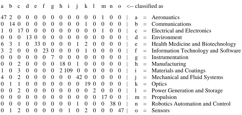
Table 10: Confusion matrix of the samples after applying SMO on iteration 2 data. ... 36
Table 11: Accuracy of the model, after multiplying the training samples in dataset ... 37
Table 12: Training sample File count before and after insertion of synthetic data ... 38
Table 13 Confusion matrix of the test samples before addition of synthetic data. ... 39
Table 14: Confusion matrix of the test samples after addition of synthetic data. ... 39
v
List of Figures
Figure 1: Hyperplane in SVM, possibility of many hyperplanes which divide the data points. ... 19
Figure 2: Hyperplane with support vectors in SVM, where the solid line represents the decision boundary
while the thin lines represents the boundaries of maximal margin area. Data points lying on the thin
lines are the support vectors. ... 20
Figure 3: Steps involved in text classification process The Experimental data is preprocessed using
unsupervised and supervised filtering techniques. Machine learning algorithms are applied on the
preprocessed data. Based on the model accuracy and training samples available in each class, synthetic
data is added and the process is repeated from stage ii. ... 25
Figure 4: Frequency distribution of "light" attribute in the documents, horizontal axis is the TF-IDF value
of the term "light", each color represents a class present in the training dataset and the value on the top
of each vertical block represents the total count of the term in the respective frequency zone. ... 31
Figure 5: Frequency distribution of "reflective" attribute in the documents... 31
Figure 6: Frequency distribution of "alkali" attribute in the documents ... 32
Figure 7: Home page of Text classification tool. After selecting file from a location, click “Submit” button
for the output. Once the prediction is completed, the output is shown in the text area present in the
window. ... 43
Figure 8: Output prediction window for Text classification tool. Once an input file is selected, it is
evaluated by the classifier model and output is predicted. ... 44
Figure 9: Probability distribution pie chart for the test instance: input file probability distribution over all
the labeled classes is shown based on the classifier evaluation. ... 45
Figure 10: Operation of tool through command line version, inputs: Application’s runnable jar file location
and a test file. ... 46
Figure 11: Operation of tool through command line version with options. For this application, we have
developed the code to provide the probability distribution of the input file when option “p” is passed
vi
Abstract
Text classification is used in information extraction and retrieval from a given text, and text
classification has been considered as an important step to manage a vast number of records given in
digital form that is far-reaching and expanding. This thesis addresses patent document classification
problem into fifteen different categories or classes, where some classes overlap with other classes
for practical reasons. For the development of the classification model using machine learning
techniques, useful features have been extracted from the given documents. The features are used to
classify patent document as well as to generate useful tag-words. The overall objective of this work
is to systematize NASA’s patent management, by developing a set of automated tools that can assist
NASA to manage and market its portfolio of intellectual properties (IP), and to enable easier
discovery of relevant IP by users. We have identified an array of methods that can be applied such
as k-Nearest Neighbors (kNN), two variations of the Support Vector Machine (SVM) algorithms,
and two tree based classification algorithms: Random Forest and J48. The major research steps in
this work consist of filtering techniques for variable selection, information gain and feature
correlation analysis, and training and testing potential models using effective classifiers. Further, the
obstacles associated with the imbalanced data were mitigated by adding synthetic data wherever
appropriate, which resulted in a superior SVM classifier based model.
KEY WORDS
Machine learning algorithms, Patent classification, imbalanced data, SVM, Multi-class
1
1.
Introduction
Document classification is the process of classifying a document into a predefined category. It
plays a vital role in managing large number of text documents by automating the document
classification task. The two main approaches in machine learning for document classification are
supervised learning [1], where the model is trained with labeled documents, and unsupervised
learning, where the predefined category or training data is not available for the classification task,
rather clusters are made to observe the natural grouping of the documents. Further, the given
document in supervised approach can be labeled as a single-class document as well as multi-class
documents. Multi-class labeled document classification is relatively challenging compared to the
single-class labeled document [2].
Supervised learning models are widely applicable because often the possible categories are
predetermined based on business activities. Document classification mainly consists of document
representation (vector form), feature selection, feature extraction, application of machine learning
algorithm on the data for evaluation.
In this study we performed classification task on NASA’s patent documents, available in html
format and downloaded from the U.S. Patent Office [3]. We applied five machine learning methods
k‐ Nearest Neighbors (kNN), two variations of Support Vector Machine (RBF and PolyKernel), and
two tree‐ based classification algorithms (Random Forest and J48), to carry out the initial
classification on NASA patent data. We have assessed the accuracies of the initial classification with
5 fold cross‐ validation. Based on the results, we conclude that the SVM performed well on the
available patent data compared to other algorithms.
Along with the classification of top level categories, we have proposed a way to further proceed
2
to which top category the document belongs. For example, a document, which is classified as
“Aeronautics”, can be further classified into “Aircraft” or “Control” depending on its content. Thus,
the sub category classification enhances user’s visual discovery of intellectual property content of
the documents.
Tag words can be generated from the training files as well as from the input files based on the
information gain [4] of the useful word or term calculated from the given document. The generation
of these tag words will provide further fine-grained details about patents combining the
subcategories information, which will assist in search activities and document management.
To perform the entire document classification and management task, we have developed the
proposed tool in Java. This tool uses the training data samples that are provided, builds model and
then predicts the category of the input document. Along with the classification, probability
distribution of the document could be viewed in pie chart by utilizing the probability values which
is generated by the classifier. This helps user predict multi-labeled document and enable to place the
document in the most appropriate category.
One of the challenges in this project was the existence of the imbalanced datasets. Imbalance in
training dataset implies significant difference in the number of samples present in the classes.
Imbalance dataset is problematic, because the total error of the majority-class biases the decision
boundary in favor of the majority class by almost masking the minority-class [5]. In such cases the
classification would tend to over adapt the classes with high number of samples ignoring the smaller
classes [6]. To overcome the problem of document classification involving imbalanced and low
training dataset, we have implemented a solution by adding synthetic data to the minority class.
The synthetic data has been collected from well‐ known [7] taxonomical repositories and articles,
3
paper we analyze the accuracy of SVM classifier with data imbalance problem in classes and also
describe how synthetic data addition to the training data set have improved the accuracy of the
4
2.
Literature Review
In this section, a relevant literature related to the proposed research work has been discussed.
2.1 Review of multi-class document classification
In a pioneering approach, Fabrizio Sebastiani mechanized automated classification (or
classification) of texts into predefined classes, this approach had seen an expanding enthusiasm in
recent years, because of the expanded accessibility of documents in digital form and the subsequent
need to classify them [8]. The predominant way to deal with these text-classification problems are
popularly and manageably done using machine learning techniques, a general inductive process that
naturally builds a text classifier by learning from a set of labeled text documents, the attributes of
the categories. The benefits of this approach over the knowledge engineering approach (manual
classification and annotation by domain specialists) are a decent viability, and direct movability to
various domains. The success story of automated text classification is expanding to neighboring
fields of application. For example, noisy text classification resulting from the optimal character
recognition and speech transcripts are available and inspiring [8].
Text classification has advanced from a minor research field in late '80s, into a completely
bloomed investigation field, which has produces proficient, powerful, and generally useful
classifications with many application areas. This achievement has been based on two aspects of
modernization: first, the continually expanding inclusion of the machine learning group in text order,
which has of late brought about the utilization of the latest machine learning innovation in text
classification applications, and second, the accessibility of standard benchmarks, (for example,
Reuters-21578 and OHSUMED) [9], which has supported research by giving a setting in which
distinct research endeavors could be contrasted with each other, and in which the best techniques
5
2.2 Review of approaches in document classification
Currently, text classification has become one of the key methods to handle and organize text data
[10]. Documents, which generally contains strings of characters, have to be transformed into a
suitable representation that usable in learning algorithms and classification problems. Information
retrieval research suggests that word stems work very well as representation units leading to attribute
value representation of text, which is used in implementing this project. The word stem is derived
from the form of a word by removing case and derived information [11]. For example “machine”,
“machining” are all mapped to the same stem “machin”. This leads to an attribute value
representation of the text data. For each unique word, its count 𝜔𝑖 in the data corresponds to a feature
as term frequency (𝜔𝑖, d), in corresponding text document d. To overcome the unnecessarily large
feature vectors, words are represented as features if they have occurred in the training data set usually
at least 3 times. Based on this representation, scaling the dimensions of the feature vector with their
respective inverse document frequency (IDF, which is applied as the log inverse of 𝜔𝑖) leads to an
improved performance. IDF is calculated from the total number of training documents (n) and the
document frequency of the particular word 𝜔𝑖 as shown in equation (1):
𝐼𝐷𝐹 (𝜔𝑖) =𝑙𝑜𝑔 ( 𝑛
𝐷𝐹(𝜔𝑖)) (1)
Here, 𝐷𝐹(𝜔𝑖) is the number of those documents in the collection, which contain the term 𝜔𝑖. Based
on the standard feature vector representation of the text data, it was argued in [3] that the support
vector machines are more appropriate for this type of setting. Different classification methods such
as Bayes, SVM, C4.5 and kNN were applied on the Reuters-21578 and Ohsumed corpus [2] among
6
Rennie Jason [12] in his work indicated that, SVMs performed better than Naïve Bayes for the
multiclass text classification problems. 20 Newsgroups is a data set collected and originally used for
text classification by [13]. Datasets from 20 Newsgroups and Industry-Sector [14, 15] were used for
the experimental setup. Empty documents that are generated after preprocessing (23 for 20
Newsgroups, 16 for Industry Sector) were filtered out. The code and pre-processed data used in
experiments can be obtained from [16, 17].It contained 19,997 documents evenly distributed across
20 classes. All headers, UU-encoded blocks, stop words and words that occur only once were
removed from further consideration. The vocabulary resulted into 62,061 words. Randomly selected
80% of documents per class for training and the remaining 20% for testing. This is the same
pre-processing and splitting as McCallum and Nigam used in their 20 Newsgroups experiments [14].
Later, the experiments were conducted on 10 fold cross-validation (FCV) [1, 18]. To gauge
performance for different amounts of training documents, the authors created nested training sets of
800, 250, 100 and 30 documents per class for 20 Newsgroups and (up to) 52, 20, 10 and 3
documents/class for Industry Sector. Empirical calculation of error for different sizes of data sets and
their classification using SVMs and Naïve Bayes are also provided. Based on the experimental
results, the support vector’s improved ability in performing the binary classification have given lower
errors compared to Naïve Bayes.
As indicated in [19], machine learning for text classification is best available tool for document
classification, news filtering, document routing, etc. In text classification, effective feature selection
is very important to make the learner model effective and more precise. Commonly known metrics
such as Chi Squared, Bi-normal Separation, Information Gain, Probability Ratio, etc. have been
applied on the data to extract the features. Information Gain (IG) measures the decrement in entropy
7
Information gain (IG): In Machine learning field Information gain is commonly employed as a
term-goodness criterion [20]. By knowing the presence and absence of a term in a document, IG
measures the number of bits of information obtained for the category prediction. Let {𝑐𝑖}𝑠𝑠𝑖=1𝑚 denote
the set of categories in target space, and the information gain of a term t is calculated as
𝐺(𝑡) = − ∑𝑚𝑖=1𝑃𝑟(𝑐𝑖)𝑙𝑜𝑔𝑃𝑟(𝑐𝑖)+𝑃𝑟(𝑡) ∑𝑚𝑖=1𝑃𝑟(𝑐𝑖/𝑡)log𝑃𝑟( 𝑐𝑖
𝑡)
+ 𝑃𝑟(𝑡̅) ∑𝑚𝑖=1𝑃𝑟(𝑐𝑖/𝑡̅) log𝑃𝑟(𝑐𝑖/𝑡̅) (2)
Here, m is the target space dimension, and 𝑃𝑟 is the probability of occurrence of term t in document
corpus. In a given training corpus, the information gain is computed for each unique term and the
terms were removed from the attribute space if the information gain is less than the predetermined
threshold value. In [20] the authors performed evaluation of feature selection techniques like IG,
Chi-squared, Document frequency thresholding, and Mutual information [20] using Reuters [21] and
Ohsumed [9] data and found Chi-squared and IG were more effective in aggressive term removal
without losing categorization accuracy.
The work [19] introduced an observational examination of twelve-element choice techniques (i.e.,
Information Gain) assessed on a benchmark of 229 text classification issue occasions that were
assembled from Reuters, TREC, OHSUMED [9], and so forth. The outcomes are investigated from
numerous objective point of view such as exactness, F-measure, accuracy, and review since each is
suitable in various circumstances. The overall feature selection procedure is to measure each
potential feature according to available metrics like Chi Squared, Bi-normal Separation, Information
Gain, and Probability Ratio and to consider the best k-features. Scoring the features involves counting
the occurrences of the feature in positive and negative class in a training datasets separately and to
8
motivated to investigate and implement the IG based approach because of its proven effectiveness
[19].
Text classification has been considered a much needed technique to oversee and handle an
nearly-unlimited amount of documents in digital forms that are far reaching and ceaselessly expanding [22].
A document can be represented as an array of words, however, not all words in a document can be
used for training the classifier, and those words to be ignored are called stop words. For example
auxiliary verbs, conjunctions, articles can be classified into stop words. In a preprocessing task, stop
words are often removed from consideration.
Stemming is another common task in preprocessing step. A stemmer algorithm replaces the words
with the same stem with their respective stem-word. The removal reduces unrealistic feature
variations, increases frequency count for the important feature and reduces the input-features
dimension. This reduction of the curse of dimensionality [1] yields in improved classification
accuracy.
Feature transformation differs significantly from feature selection approaches however, like
feature selection, its main purpose lies in reduction of feature set size. Principal component analysis
(PCA) is a famous approach used for the feature transformation [23]. The aim of the usage of PCA
is to generate a discriminative transformation matrix to reduce the initial feature space into a lower
dimensional feature space which reduces the complexity of the classification without any (zero to a
little) trade off in accuracy as a choice. Feature extraction or feature selection techniques like term
frequency, inverse document frequency, information gain described in this paper are followed in the
preparation of our data.
As indicated by John Platt [24], in his new algorithm for the training of support vector machines:
9
classification of a huge quadratic programming (QP) improvement issue. SMO breaks this vast QP
issue into a progression of smallest conceivable QP issues. These small QP issues are tackled
analytically, which abstains from utilizing a tedious numerical QP enhancement as an inner loop.
The measure of memory required for SMO is directly dependent on the preparation set size, which
permits SMO to deal with large training sets. The data set used in the experiment to test SMO’s speed
was the UCI "adult" data set, which is available at [25]. The SVM was given 14 attributes of a census
form of a household. The training times of SVM and chunking algorithm were compared on the data
set. SMO’s time scales for the training order is comparatively better than the chunking time. SMO's
computation time is mainly dominated by evaluation of SVM subsequently, SMO is faster for linear
SVMs and scanty information sets. On real world data, SMO can be more than 1000 times quicker
than the chunking algorithm. This motivates us to apply SMO classifier setting to perform the
classification task in our project.
Aurangzeb Khan et al. [26] reviewed a few machine learning approaches and text classification
strategies. Data preprocessing is done using feature extraction and feature selection approaches. In
feature extraction, stemming, tokenization, stop words removal is applied on the documents. After
feature extraction, vector space is constructed using the Term Frequency/Inverse Document
Frequency (TF-IDF) approach. TF-IDF captures relevancy among the words, text documents and
particular categories. The statistics from information gain and chi square confirms that these are the
mostly used and well performed techniques for feature selection. More than 100 variants of five
major feature selection methods are tested using four popular classification algorithms: Naive
Bayesian (NB) approach, Rocchio's-style classifier, kNN technique and Support Vector Machines.
Among all the machine learning algorithms, Support Vector Machine, Naïve Bayes, kNN and their
10
literature. NB algorithm performed well in spam filtering and email classification or categorization,
which requires a small amount of data for training to calculate the parameters useful for
classification. On the other hand, SVM method was able to effectively collect the inherent
characteristics and embed the structural risk management principle which reduces the upper bound
on the generalization error. However, the main disadvantage of SVM lies in difficulty of parameter
tuning and selection of kernels.
Support vector machines (SVMs) were initially intended for binary classification of documents
[27]. Step by step the algorithm has been extended for multiclass classification. A few strategies have
been proposed where a multiclass classifier is built by combining many other binary classifiers [28].
Some researchers have proposed strategies that consider all the classes at once. The authors
compared the methods performance and three techniques based on binary classifications:
"one-against-all, “one-against-one," and coordinated non-cyclic diagram SVM (DAGSVM). Their tests
show that the "one-against-one" and DAG techniques are more reasonable for pragmatic use than
alternate methods. From UCI Repository [29] the following datasets: iris, wine, glass, and vowel
were collected. From Statlog collection [29], all multiclass datasets: vehicle, segment, dna, satimage,
letter, and shuttle were collected. The data sets were trained using RBF kernel 𝐾(𝑥𝑖, 𝑥𝑗) ≡
𝑒−𝛾||𝑥𝑖−𝑥𝑗||2 parameters. The generalized accuracy is measured using different kernel parameters 𝛾
and cost parameters C: 𝛾 = [24,23,22,…2-10] and C=[212,211,210,…2-2]. From these experimental
results, authors concluded that the SVMs accuracy could be increased by changing the kernel and
cost parameters.
As indicated by Simon Tong [30], text classification have a vital role to play due to the recent
expansion of readily available data. SVMs have gained remarkable success in solving number of real
11
In this work, authors represent the document as a stemmed, TD-IDF-weighted word frequency
vector. Stop word consisting of list of common words were used to ignore the irrelevant features.
Because of proven significance, stop words and TD-IDF preprocessing techniques are implemented
in our project.
As indicated by Edda Leopold [32], the decision of the kernel function is critical to most
applications of support vector machines. Representation of texts in input space is performed by
frequency transformations and inverse document frequency. In frequency transformation the term
frequencies 𝑓(𝑤𝑘, 𝑡𝑗) is used and multiplied with inverse document frequency. IDF of term in a
text data collection consisting of N document is calculated suing equation (1). The vector of the IDF
for all types in the document collection is given by
𝐼𝐷𝐹=(𝐼𝐷𝐹1, … 𝐼𝐷𝐹𝑛) (3)
Thus, the product of frequency transformation and the IDF gives the vector of the text to be
represented in the input space. Test input data were collected from Reuters-21578 dataset,
Frankfurter Rundschau newspaper and Die Tageszeitung (German) newspaper [21]. SVM classifier
with linear, polynomial and RBF kernel were applied on the data. The experimental results have
shown that the kernel functions did not affect the precision and recall performance very much.
Compared to polynomial and linear kernels, RBF kernel generated more support vectors. The
experimental results have also shown that SVMs are capable of efficiently processing very high
dimensional feature vectors.
According to Kim [33], Support vector machines (SVMs) have been perceived as a standout
amongst the best classification strategies for some applications including text categorization. The
experimental data consists of a subset of MEDLINE database [34] with 5 categories. Each class has
12
algorithms for dimensionality reduction of clustered data: For term document matrix A, the reduced
dimensional representation is achieved by transforming each document vector in the m dimensional
space to a vector in the l dimensional space for some l < m. Dimensional reducing transformation GT
∈ 𝑅𝑙×𝑚 is computed explicitly or the dimensionality can be achieved by formulating as a rank
reducing approximation where the given matrix A is decomposed into two matrices Y and B i.e.
𝐴 ≈ 𝐵𝑌 (4)
Here, 𝐵 ∈ 𝑅𝑙×𝑚 with rank (B) = l and 𝑌 ∈ 𝑅𝑙×𝑛 with rank (𝑌) = l.
The optimal separating hyperplane of one versus rest binary classifier could be obtained by
conventional SVMs. The decision rule for SVM is
𝑦(𝑥, 𝑗) = 𝑠𝑖𝑔𝑛 ( ∑ 𝛼𝑖 𝑥𝑖∈𝑆𝑉
𝑦𝑖𝐾(𝑥, 𝑥𝑖) + 𝑏 − 𝜃𝑗𝑆𝑉𝑀) (5)
Here y (x,j) ∈ {+1, -1} is the classification for the document x with respect to the class j, SV is the
support vectors set, 𝜃𝑗𝑆𝑉𝑀 is class specific threshold for the binary decision, ∑𝑛𝑖=1𝛼𝑖𝑦𝑖 = 0, 0 ≤
𝛼𝑖 ≤ 𝐶, 𝑖 = 1, . . 𝑛 and the kernel function is represented with 𝐾(𝑥, 𝑥𝑖) =< ∅(𝑥𝑖), ∅(𝑥𝑗) > where <,
> represents the inner product of two vectors, is introduced to handle nonlinearly separable cases
without any explicit knowledge of the feature mapping ∅. This threshold is set so that a new
document x should not be classified to belong to class j when it is located very close to the optimal
separating hyperplane. After performing classification using algorithms like SVM and kNN, it was
shown that the classification accuracy of the SVM is higher and it achieved a significant reduction
in the time and space complexity. Despite the fact that the learning capacity and computational
complexity of training in support vector machines might be independent of the dimension of the
13
a large number of terms in solving the text classification problems. Novel dimension reduction
strategies to lessen the dimension of the text vectors drastically were implemented. Decision
functions for the classification algorithm and support vector classifiers to deal with the classification
issue where a text document may have the probability of belonging to multiple classes were
presented. The significant exploratory results in the paper demonstrate that several dimension
reduction strategies that are composed particularly for clustered data, higher efficiency for both
training and testing can be accomplished without giving up prediction accuracy of text categorization
even when the dimension of the input space is essentially decreased [33].
2.3 Overcoming data imbalance issue
According to R. Longadge et al. [5], imbalance data set is the greatest problem in data mining
[35]. The authors have proposed three methods for classification of imbalance data set which is
divided into three categories namely algorithmic, data preprocessing and feature selection approach.
The paper demonstrates systematic study of these approaches and the right direction for the class
imbalance (class imbalance occurs when one of the two classes having more sample than other
classes) problem. Sampling methods are used in solving the data imbalance problems, which is
known as data preprocessing method. Under-sampling and oversampling are the two methods
described in this paper. The authors provided the methods to perform the feature selection and
algorithmic approaches and concluded that the data preprocessing method provides much better
solution than other methods as it allows the addition of new data into the existing data or the deletion
of the redundant data, which is of less importance. Under-sampling is an efficient strategy to deal
with class imbalance but the drawback of under sampling is that it loses many potential data as some
14
information loss from the majority class, both k-means algorithm and random sampling approaches
were implemented to generate balanced data sets.
𝑆𝑖 = 𝑋𝑀𝑖𝑛×𝑅𝑖, 1 ≤ 𝑖 ≤ 𝑘 (6)
Here, 𝑅𝑖 = 𝑋𝑀𝑎𝑗_𝑖/𝑋𝑀𝑎𝑗 for 1 ≤ i ≤ k, 𝑋𝑀𝑎𝑗 is majority class samples, 𝑋𝑀𝑖𝑛 are minority class
samples and 𝑋𝑀𝑎𝑗_𝑖 is the majority of samples in the ith cluster. The following algorithm 1 is proposed
for implementing under-sampling technique.
Algorithm 1: Implementation of under-sampling technique.
INPUT: Majority class samples, minority class samples.
OUTPUT: Balanced training set
Step1: Cluster all the majority class samples into k clusters using k-means clustering.
Step2: Compute the number of selected majority class samples in each cluster by using equation
(6) and select Si majority samples in ith cluster. This is done by selecting Si majority class samples
in ith cluster randomly. Thus, majority sample subsets C is obtained.
Step3: Combine C with all the minority class samples respectively to obtain the training set B.
The proposed approaches are tested on UCI data sets [29] and found that kNN has improved
performance compared to SVM. According to the experimental results, SVM’s performance
degraded as the class imbalance increased.
According to Rehan [36], SVM has been widely considered and has indicated noteworthy
accomplishment in numerous applications. The accomplishment of SVM is extremely constrained
when it is applied to the problem of learning from imbalanced datasets in which negative cases
intensely dwarf the positive cases (e.g. in gene profiling and distinguishing credit card fraud).
15
approaches applied for imbalanced data sets. A new algorithm which needs to bias SVM in a way
that will push the boundary away from the positive instances is introduced. The performance of
proposed algorithm against the SMOTE algorithm by Chawla et al., consolidated with Veropoulos
et al.'s different error costs calculation, alongside under-sampling and general SVM, demonstrate
that the proposed algorithm works well. The main problem with imbalanced data sets is that they
skew the boundary towards the minority class instances. The classification function for the hard
margin linear SVM is as follows:
𝑆𝑖𝑔𝑛((𝑤. 𝑏) + 𝑏) (7)
Here, 𝑤 is a vector that is normal to the separating hyperplane. The norm of w and variable b decide
the distance of the hyperplane from the origin. This skew of the learning hyperplane is tested on UCI
datasets [29]. Ideal boundary for this dataset is measured by testing balanced datasets which are
linearly separable and noise free in the feature space. When SVM classifier is applied on the balanced
UCI data [29], 100% accuracy is achieved. Upon repeating the experiment by keeping the positive
instances same and reducing the negative instances, the results have shown a significant angles
between ideal and learned hyperplane. Thus, this motivates us to reduce the data imbalance issue in
our training set, while applying SVM with a good faith.
According to Yanling Li, Guoshe Sun, Yehang Zhu [6], imbalance in training data set means a
significant difference in the number of samples present in the classes. In such cases the classification
would tend to over adapt the classes with high number of samples ignoring the smaller classes. In
most of the text classification problems this data imbalance is common. For example in monitoring
the public opinion data, information security and supervision, most of the cases the quantity of texts
which holds a negative view will be very low compared to the positive views. Classification
16
imbalanced data sets. Their paper mainly focused on analyzing different forms of data imbalances
including text distribution, class overlap, and class size and devised the conclusions based on
experimental values.
3.
Preliminary Work
3.1 Approaches to document classification using machine learning
In supervised approach, single-label documents are those which are classified into one class only,
multi-label documents are those which are classified into more than one class [2]. In this project we
perform multi class classification, in which a file is predicted into one of the predefined categories.
Supervised learning models are widely applicable and can offer the insight about how the
explanatory variables are related to the categorical response variable. Document classification
mainly consists of document representation (vector form), feature selection, feature extraction,
application of machine learning algorithm on the data for evaluation. There are different types of
supervised text classification techniques available in machine learning platform, which we applied
to perform our preliminary assessment discussed below:
kNN (k Nearest Neighbors): kNN algorithm is based on the assumption that the classification of
a document is analogous to the classification of the other documents that are nearby in the vector
space. “k” in kNN is a user-defined constant which is used to find the most frequent label of k
training samples (documents) nearest to the unlabeled vector or test document.
Support Vector Machines: It is a supervised classification algorithm which is extensively
implemented in text classification problems. SVM have the potential to handle large feature spaces
as they use over fitting protection which does not depend on the number of attributes [37]. The task
17
Random Forest: It is a robust and versatile algorithm, which is used for classification of
documents. Random forest consists of many individual trees [38]. In this method, each tree votes on
an overall classification for the given dataset and the random forest algorithm choses the most voted
individual classification.
J48 Decision Trees: A decision tree is a predictive machine learning model which decides the
target value of a new sample based on several attribute values of the available training dataset. A
binary tree is created based on the training dataset and it is applied to target instance in the dataset
for the classification.
We applied five machine learning methods on the experimental data [3] to carry out the initial
classification. These five methods are k‐ Nearest Neighbors (kNN), two variations of Support
Vector Machine (SVM), and two tree‐ based classification algorithms Random Forest and J48. We
have assessed the accuracies of the initial classification with 5 fold cross‐ validation. The
following Table shows training accuracies obtained from various methods using the full‐ text
documents:
Table 1: Comparison of five machine learning methods’ training accuracies for the given 15 categories.
kNN
(w/ k=9)
SVM (w/RBF‐kernel)
J48 Random Forest SVM
(w / PolyKernel exp (1.0))
54% 55.4% 57.07% 61.04% 69.2%
Based on the results from the above table, we have proceeded with SVM classifier algorithm to
make the classification tool more robust for this experimental setup, because, in our preliminary
18
3.2 A Dissection of Support Vector Machine in Classification
Support Vector Machines is a classifier formally defined by a separating hyperplane in other
words, given labelled training data (supervised learning), the algorithm outputs categories. SVM is
a relatively new class of machine learning techniques first introduced by Vapnik [37] and has been
introduced in Text classification by Joachims. The Support vector machine classifier needs both
positive and negative training set, which are uncommon for other classification problems. These
positive and negative training set are needed for the SVM to seek for the decision boundary that
separates the two classes in the n dimensional space, so called the hyperplane. The documents, which
are closest to the decision surface, are called the support vectors. The accuracy or efficiency of the
Support vector machine classifier classification does not alter if documents that do not belong to the
support vectors are removed from the set of training data.
Usually the classification problem can be confined to thought of consideration of the two-class
(binary) problem without loss of generality. The main goal of the problem is to separate the two
classes by a function which is induced from available examples. The goal is to produce a classifier
that will work well on unseen examples. Consider the example in Figure 1. In the figure there are
many possible linear classifiers that can separate the data points, but there is only one classifier that
maximizes the margin (maximizes the distance between it and the nearest data point of the two
classes). Such linear classifier is defined as the optimal separating hyperplane. Intuitively, we would
19
Figure 1: Hyperplane in SVM, possibility of many hyperplanes which divide the data points.
The goal of SVM is to maximize the margin in-between classes of the training data. It implies
finding the biggest margin provides the optimal hyperplane for the classifier. A hyperplane separates
the two classes based on the equation (8).
𝑤. 𝑥 + 𝑏 = 0 (8)
With 𝑤. 𝑥𝑖 + 𝑏 ≥ 1 𝑖𝑓 𝑦𝑖 = 1 and 𝑤. 𝑥𝑖 + 𝑏 ≤ −1 𝑖𝑓 𝑦𝑖 = −1 for 𝑖 = 1,2, … 𝑁
The goal of SVM is to find the optimal separating hyperplane by maximizing the distance between
the two classes, which can be calculated from equation (9).
𝑚𝑖𝑛 (1
20
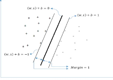
Figure 2: Hyperplane with support vectors in SVM, where the solid line represents the decision boundary while the thin lines represents the boundaries of maximal margin area. Data points lying on the thin lines are the support vectors.
3.3 Attribute Selection
Attribute selection plays a key role in data preparation for training the classifier model. It is a
process in which the best set of attributes are selected from the dataset. It is used to create transforms
of the dataset such as rescaled attribute values into their constituent parts to make more and useful
structure for the classifier models. Keeping irrelevant attributes in the training model could cause
overfitting problem.
Tokenization: Text data available is composed of terms grouped into sentences and paragraphs.
One technique to represent text data using the vector space model breaks down the textual data into
a set of terms. Each of these terms corresponds to an attribute of the input data and therefore becomes
21
to the terms contained in the data collection and whose value indicates either a binary present/absent
value or a weightage for the term for the data point. This representation is known as the Extracted
Term' representation and is the most commonly used representation for text data patterns. The
process of breaking the available stream of text into words is called tokenization.
Feature extraction using StringToWordVector: This filtering method transforms string attributes
present in the text document into word vectors i.e., creates one attribute for each term that is present
in the document. The filtering options for applying on the dataset are discussed in section 3.4.
Information Gain Attribute Evaluator (InfoGainAttributeEval): Once the feature extraction is
completed, feature selection is implemented by using the Attribute Selection filter. Information Gain
Attribute Evaluatorpresent in the filter allows us to set the threshold of the weights of the features
to be selected for classification. In our project we have set the threshold to 0.0 such that all the
features with positive information gain are taken into consideration.
3.4 A Machine Learning Toolkit, WEKA
Weka tool is a collection of machine learning algorithms for the data mining/document
classification tasks. The algorithms could be applied to the datasets directly or called from user
developed java code. This application contains data pre-processing, classification, regression,
clustering etc. and many other tools. It is well-suited for developing machine learning schemes and
applications. [39]
The following options that are available in StringToWordVector filter are used for preprocessing
the training data set. The method executes used to normalize the reiterations to get the multi-terms
extraction.
22
wordsToKeep - The number of words (per class if there is a class attribute assigned) to attempt to
keep.
outputWordCounts - Output word counts rather than Boolean 0 or 1 (indicating presence or absence
of a word).
lowerCaseTokens - Set to make all the word tokens to converted to lower case before being added to
the dictionary.
normalizeDocLength - Sets the word frequencies for a document (instance) to be normalized.
TFTransform – TF stands for Term Frequency. TFTransform sets the word frequencies to be
transformed into:
log(1+fij) (10)
Here, fij is the frequency of word i in document (instance) j.
IDFTransform – IDF stands for Inverse Document Frequency. IDFTransform sets the word
frequencies in a document to into:
fijlog (num of Docs/num of Docs with word i),
(11)
Here fij is the frequency of word i in document (instance) j.
Term weighting plays vital part in the determination of the success or failure of classification
problems. As every term has different level of weightage in a text document, the term weight is
associated with every term as an important factor. Term frequency of each word in a document (TF)
is a weight which relies on the distribution of each word in text documents. Term frequency can be
calculated from the equation (10) and it describes the weightage of the word in the given text
document. Inverse document frequency of each word in the document database (IDF) is a weight
which relies on the distribution of each word in the document database. It is calculated using equation
23
word to determine how well the word describes an individual document within a corpus. It does this
by weighting the term positively for the number of times the term occurs within the given document,
while also weighting the term negatively relative to the number of documents which contain the
word. Consider term t and document d, where t occurs in n of N documents in D. The TF-IDF
function is of the form:
TFIDF(t, d, n,N) = TF(t, d) × IDF(n,N) (12)
TF-IDF approach is run against all terms in all documents in the document corpus to rank the
words by their weights. Higher TF-IDF weight indicates that a word is both important to the
document, as well as relatively uncommon across the document set. This is often interpreted to imply
that the term is significant to the document, and could be used to accurately summarize the document.
TF-IDF provides a good heuristic for determining likely candidate keywords. TF-IDF approach is
very popular in text classification field and almost all the other weighting schemes are variants of
this approach. In vector space model organization of document also affect the performance of system.
In this experiment we use term frequency method and inverse document frequency for our
experiment setup options.
Applying Snowball Stemmer:
This algorithm reduces inflected/derived words to their word stem, by trimming the root of its
inflectional affixes; usually, only suffixes that have been added to the right-hand end of the root word
are removed. It reduces the repetitions of words of the same form which gradually reduces the
dimensionality of the word vectors.
Removing Stop words using Rainbow list:
Stop words, are the words, which are filtered out prior to the processing of natural language data
24
classification. They are usually defined as functional-words, which do not carry meaning and
influence the classification positively. In our setup, we use rainbow stop words list and have
appended them with extra words to make the list effective. Thus by the removal of these stop words,
25
4.
Methods and their Integrations
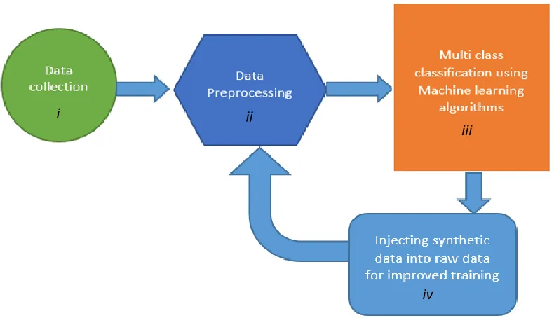
Our experimental setup consists of the following 4 stages and the information flow has been shown
by Figure 3:
i) Experimental Data Collection
ii) Data Preprocessing
iii) Applying Machine Learning algorithms
iv) Synthetic data Injection
The Experimental data is collected and preprocessed using StringToWordVec and
AttributeSelection filters. Once the data is preprocessed, the model is trained with the data.
Depending on the accuracy of the model obtained using cross fold validation, synthetic data is added
to the required classes and the process is repeated from stage ii.
Figure 3: Steps involved in text classification process The Experimental data is preprocessed using unsupervised and supervised filtering techniques. Machine learning algorithms are applied on the preprocessed data. Based on the model accuracy and training samples available in each class, synthetic data is added and the process is repeated from stage ii.
i
iv ii
26
Stage 1. Experimental Data Collection
By manual processing, a team of NASA experts identified 15 top-level categories for their
patents. The information about these patents is available online. By selecting one of these categories,
the NASA’s (intelligent properties) portfolio is capable of restricting the results within the chosen
category. However, improvement is needed. For example, the precision of the search results of
“social network” is only 4.2%; out of 24 output items (descriptions of patents), 23 are irrelevant but
included due to the word “network”. On the other hand, the relevant item is categorized under
“Health, Medicine and Biotechnology”. Finding the relevant item through category-by-category
search will take time because the logical relationship between “social network” and “Health,
Medicine and Biotechnology” is not obvious. The problem of this example can be effectively solved
by refined categorization and semantic tagging.
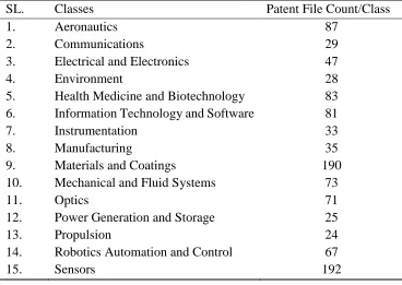
Table 2: Number of training documents available in the experimental data.
SL. Classes Patent File Count/Class
1. Aeronautics 87
2. Communications 29
3. Electrical and Electronics 47
4. Environment 28
5. Health Medicine and Biotechnology 83 6. Information Technology and Software 81
7. Instrumentation 33
8. Manufacturing 35
9. Materials and Coatings 190
10. Mechanical and Fluid Systems 73
11. Optics 71
12. Power Generation and Storage 25
13. Propulsion 24
14. Robotics Automation and Control 67
15. Sensors 192
In the experimental data, each patent document were assigned category and were classified into
27
that majority of the manually assigned classes to the patent files were correct; but some files could
be misclassified. Further, some files could be qualified for more than one classes but only one class
has been assigned.
Challenges faced in experimental data
Presence of less informative sections in patent files: Consider the “References” section in a patent
document, which does not provide positive information about the document.
Solution: Every section of patent file in the experimental data is not useful for training. Hence,
extracting features from the “References” section of a patent document merely increases the
dimensionality of the space rather than providing useful information. Thus some sections like,
“References”, “See also” etc. were removed from the files, which deliberately provides useful words
for training the classifier.
Data Imbalance issue: The number of training samples for each class in the experimental data set
if not consistent. For example, there is huge difference in the samples count of Sensors class and
Power Generation and Storage class.
Solution: The classifier model tends to bend towards the Sensors class due to more number of
Support vectors generated by Sensors. To resolve this issue we implemented Synthetic data addition
to the classes, which contain relatively less number of training samples. Also, when the data sets are
very small, this approach helps in increasing the training material for the model i.e., the number of
attributes/features helpful for the classification are increased and also the classifier will be able to
28
Stage 2: Data Preprocessing
Creating Attribute-Relation File Format (ARFF) file: Weka tool accepts ARFF file format to
preprocess the data to perform classification. The text documents in the experimental data were
converted into ARFF format. An ARFF file is an ASCII text file that describes the list of instances
sharing a set of attributes. ARFF files have two different sections. First section consists Header
information and the second section contains data information [40]. The following command has
been used to convert the text directory into ARFF file:
Once the patent files are converted into ARFF file, it is preprocessed and used for preparing training
file for the classifier. The data preprocessing techniques used in this project are discussed in the
following sections.
Filtering options: This module processes the texts of the text database are extracted into a set of
unigrams (words) that will be used to train the classifier model. It implements two preprocessing
methods as follows, and it’s the attribute extraction phase.
Applying filters on the data
i) Unsupervised filter
ii) Supervised filter
Here, unsupervised filter StringToWordVector is applied on the data, it converts String attributes into
a set of attributes representing the word occurrence information from the text contained in the strings.
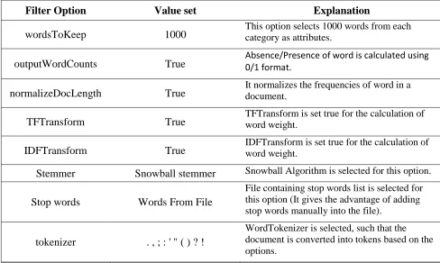
StringToWordVector filtering options applied for data preprocessing: The options shown in
Table 3 can vary depending on the size of the data. The number of attributes generated after applying
StringToWordVector filter is 4855 words. Once the StringToWordVec filter is applied on the data,
29
(hence, this is unsupervised filtering). To view the attributes in sorted order of information gain,
Attribute selection filter is applied on the generated attributes from unsupervised filter.
Table 3: Unsupervised filtering options applied on data in the experimental setup.
The Table 4 shows the options to be set in AttributeSelection filter. The number of attributes
generated after applying Attribute Selection filter is 1218. The Table 5 shows the weights and
attributes after applying supervised filter on the data. The attributes are ranked in descending order
of their TF-IDF weights.
Table 4: Supervised filtering options applied on data in the experimental setup.
Filter Option Value set Explanation
Evaluator InfoGainAttributeEval Attributes are selected based on the information gain ratio.
Search Ranker
Threshold value is set to 0.0, such that all attributes with positive information gain is considered.
Filter Option Value set Explanation
wordsToKeep 1000 This option selects 1000 words from each category as attributes.
outputWordCounts True Absence/Presence of word is calculated using 0/1 format. normalizeDocLength True It normalizes the frequencies of word in a document.
TFTransform True TFTransform is set true for the calculation of word weight.
IDFTransform True IDFTransform is set true for the calculation of word weight.
Stemmer Snowball stemmer Snowball Algorithm is selected for this option.
Stop words Words From File
File containing stop words list is selected for this option (It gives the advantage of adding stop words manually into the file).
tokenizer . , ; : ' " ( ) ? !
30
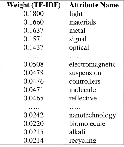
Table 5: Weight (TF-IDF) - Attributes after supervised filtering
Weight (TF-IDF) Attribute Name
0.1800 light 0.1660 materials 0.1637 metal 0.1571 signal 0.1437 optical ….. …..
0.0508 electromagnetic 0.0478 suspension 0.0476 controllers 0.0471 molecule 0.0465 reflective
….. …..
0.0242 nanotechnology 0.0220 biomolecule 0.0215 alkali 0.0214 recycling
Thus, attributes that does not contribute much to the document classification are omitted using
the above techniques. The threshold values in supervised filter can be changed based on the number
of attributes required. The flowing figure shows the frequency distribution of “light” attribute in the
documents. We can see from the figure that there is even distribution of the term “light” count in
each class (see column wise, i.e. for a particular frequency range, the count of the term is displayed
in each column per class), which makes clear that the term provides high information gain for the
31
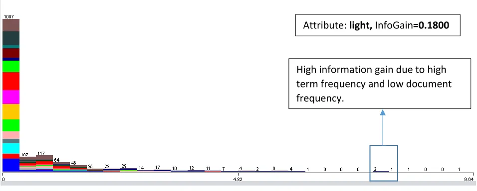
Figure 4: Frequency distribution of "light" attribute in the documents, horizontal axis is the TF-IDF value of the term "light", each color represents a class present in the training dataset and the value on the top of each vertical block represents the total count of the term in the respective frequency zone.
In the above figure we observe that the number of classes that have the term “light” are 2, with frequency
approximately in between 6-7. With high term frequency and low document frequency, the
TermFrequency-InverseDocumentFrequency (TF-IDF) is high which indicates high information gain for the
word “light”.
Figure 5: Frequency distribution of "reflective" attribute in the documents
Attribute: light, InfoGain=0.1800
Attribute: reflective, InfoGain=0.0465
32
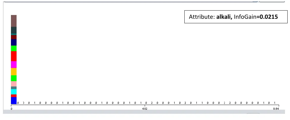
Figure 6: Frequency distribution of "alkali" attribute in the documents
Supervised filtering consists of applying Attribute selection filter on the data which extracts the
attribute based on the threshold level that is set in the filter options. This reduces the number of
attributes used for the classification. Hence words which provide more information required for the
classification are extracted. Once the data preprocessing is completed, the ARFF file is saved and
used in the preparation of model. From figures 4, 5, 6 we can see the variation of TF-IDF with the
number of documents, the term is present. In figure 4, we see that the information about the class can
be obtained more compared to figure 5, 6.
Stage 3. Applying Machine Learning algorithms for classification
Text classification is a task of deciding whether a document belongs to any of a set of pre -defined
categories based on the probability. This module implements the Classification process to perform
the classification based on the generated knowledge or training data using the Support Vector
Machine Classification Approach, the generated output for the NASA patent classification. We used
NASA’s predefined patent documents as training data for performing classification. Implementation
steps were discussed in the following section.
33
Applying algorithms experimental data: The results from Table 1 suggest that the current data,
without refinement cannot be used to build up a robust classifier. For example, kNN is a simpler
method and the poor accuracy (54%) indicates that there are many overlapped samples or, miss‐
labeled samples exist. On the other hand, SVM with various parameters, can very efficiently fit the
(augmented) data‐ space, once the given sample are consider the ground‐ truth – however, which is
not true in this case and the accuracy is not very high (~70% using SVM). Further, the tree based
approaches (Random Forest, J48) which are usually good for noisy data are not even providing good
accuracy either. Therefore, we planned to identify the good sample to determine the natural and
effective class‐ boundaries using simpler method – the simpler method, such as kNN, will help us
avoid over‐ fitting (SVM or, Tree based approach can over‐ fit easily).
Robust Training and Testing: To arrange robust and effective training using kNN approach, we
implemented the following two steps:
(1) Identify the best k value in the kNN approach (see Table 6 and 7),
(2) and iteratively retrain and remove the miss‐ classified sample and obtain best training
accuracy.
Table 6: Comparison of the training accuracies using 5 fold CV with different values of k from 1 to 10.
k = 1 2 3 4 5 6 7 8 9 10 accuracy% 60.11 54.98 55.63 55.82 54.70 54.98 55.35 54.14 53.96 55.07
Table 7: Comparison of the training accuracies using 5 fold CV with different values of k from 11 to 20.
34
We exhaustively computed the classification accuracy, for k = 1 to 20, and there is lesser
variations among the outcomes. We avoid selecting k = 1, because k = 1 by nature mostly over-fits,
hence avoidable. Thus, we selected the most reasonable as well as optimal value, k = 7.
Iteratively retrain and remove the miss‐ classified sample and obtain best training accuracy: This
is the most important step to retain the best samples and retrain using appropriate sample for higher
accuracy. This is also a very effort intensive steps, as for each iterations, we had to remove the
misclassified files applying semi‐ automatic approach. The confusion matrix and the accuracy in
each steps are shown below. It is to be noted that the accuracy is usually expected to be increasing
in each steps – however, it can degrade while there are very insufficient sample for a class or classes,
or, the samples among classes become heavily imbalanced:
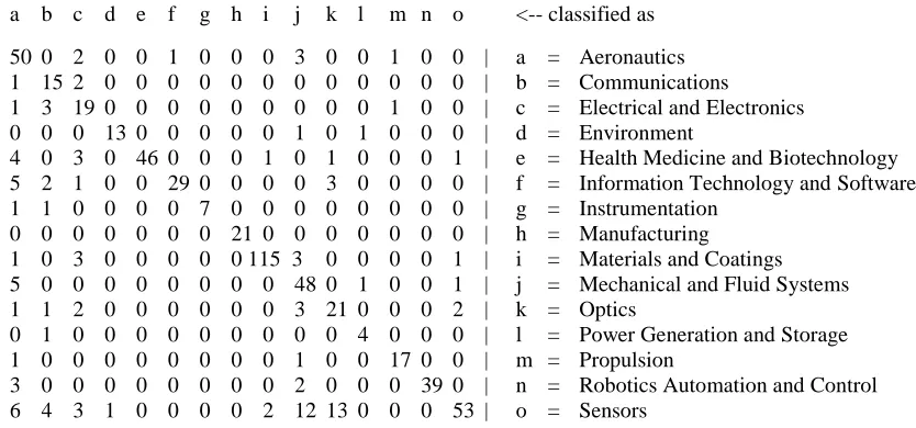
Iteration # 1: kNN (k = 7), accuracy 81.47%, this is achieved by removing miss‐ classified
samples 1st time (shown in Table 8).
Table 8: Confusion matrix of the samples kNN Iteration 1.
a b c d e f g h i j k l m n o <-- classified as
50 0 2 0 0 1 0 0 0 3 0 0 1 0 0 | a = Aeronautics
1 15 2 0 0 0 0 0 0 0 0 0 0 0 0 | b = Communications
1 3 19 0 0 0 0 0 0 0 0 0 1 0 0 | c = Electrical and Electronics
0 0 0 13 0 0 0 0 0 1 0 1 0 0 0 | d = Environment
4 0 3 0 46 0 0 0 1 0 1 0 0 0 1 | e = Health Medicine and Biotechnology
5 2 1 0 0 29 0 0 0 0 3 0 0 0 0 | f = Information Technology and Software
1 1 0 0 0 0 7 0 0 0 0 0 0 0 0 | g = Instrumentation
0 0 0 0 0 0 0 21 0 0 0 0 0 0 0 | h = Manufacturing
1 0 3 0 0 0 0 0 115 3 0 0 0 0 1 | i = Materials and Coatings
5 0 0 0 0 0 0 0 0 48 0 1 0 0 1 | j = Mechanical and Fluid Systems
1 1 2 0 0 0 0 0 0 3 21 0 0 0 2 | k = Optics
0 1 0 0 0 0 0 0 0 0 0 4 0 0 0 | l = Power Generation and Storage
1 0 0 0 0 0 0 0 0 1 0 0 17 0 0 | m = Propulsion
3 0 0 0 0 0 0 0 0 2 0 0 0 39 0 | n = Robotics Automation and Control