THE POSSIBILITIES OF CO2 EMISSION REDUCTION IN THE PROCESS OF STEEL CHARGE HEATING THROUGH THE SELECTION OF HEATING RATE

(1)

17

Research Journal

Volume 9, No. 27, Sept. 2015, pages 17–22

DOI: 10.12913/22998624/59079 Research Article

Received: 2015.07.18 Accepted: 2015.08.05 Published: 2015.09.01

THE POSSIBILITIES OF CO

₂

EMISSION REDUCTION IN THE PROCESS OF

STEEL CHARGE HEATING THROUGH THE SELECTION OF HEATING RATE

Barbara Halusiak1_{, Marian Kieloch}1_{, Jarosław Boryca}1_{, Agnieszka Benduch}1

1_{Department of Industrial Furnaces and Environmental Protection, Faculty of Production Engineering and}

Materials Technology, Czestochowa University of Technology, Al. Armii Krajowej 19, 42-200 Częstochowa, Poland, e-mail: [email protected]

ABSTRACT

The reduction of carbon dioxide emission is an important aspect of the economic policy of each country. Institutions promoting environmental protection seek to re-duce the level of greenhouse gas emissions. One of the main emitters of harmful gases to the atmosphere is the steelmaking sector. The heating technology used in metallurgical works contributes to the amount of emitted carbon dioxide that forms as a result of the loss of steel and the combustion of fuel, whose thermal energy is used during the course of the charge heating process in the heating furnace. Achieving the imposed ecological targets by not exceeding the specified emission level is possible by implementing appropriate pollutant emission reducing technologies in the metal-lurgical industry. Based on numerical computation results, the effect of heating rate on the emission of carbon dioxide has been determined in the paper. This study demon-strates that by selecting the appropriate steel charge heating technology the emissions of greenhouse gases can be substantially reduced.

Keywords: CO2 emission, heating of charge, heating technology, heating up rate,

numerical modelling.

INTRODUCTION

An important regulatory issue in environ-mental protection is the economic instrument of a State’s ecological policy in a form of transfer-able emission allowances. The operation of this mechanism consists of specifying the allowable level of emission in a given area and allocating allowances for this emission to the emitters by the institution responsible for environmental protec-tion, and subsequent trading these allowances by the emitters with one another.

The main cause of the increase in the emis-sions of greenhouse gases, and especially carbon dioxide, is sought in metallurgical processes tak-ing place in the steelmaktak-ing sector [5, 6].

Since 2005 the Community Greenhouse Emissions Trading Scheme has been functioning in the European Union. The Scheme has covered the operators of installations associated with the

generation of energy; production and process -ing of nonferrous metals; production of cement clinker, glass and ceramic products; and wood production [5].

(2)

Advances in Science and Technology Research Journal Vol. 9 (27) 2015

18

The implementation of regulations on the standards for emissions from installations for metallurgical enterprises encourages the pro-ecological investment projects to be carried out, but also creates the need for purchasing addition-al carbon dioxide emission addition-allowances, which contributes to the increase in competitiveness in the steelmaking sector [5]. It is noteworthy that by using appropriate greenhouse gas reduction technologies, the steelmaking industry could achieve the ecological goal of not exceeding the specified emission level. This paper shows how the selection of the appropriate steel charge heating technology can contribute to the reduc-tion of the carbon dioxide emission.

THE OBJECT OF MODELLING

The object of modelling is a pusher heating furnace (Figure 1) [3]. It was assumed that the heating chamber of the furnace was represented by a rectangular prism with a length of L = 28 m, a height of 2H = 2.6 m, and a width of B = 5.6 m. Also, the furnace was conventionally divided into 20 calculation zones and 5 technological zones [1, 2].

For computation purposes, the pusher fur-nace was reduced to a simple model, in which the charge moves along the furnace chamber over the length L with uniform motion counter-currently to the direction of furnace gas move-ment. It was assumed that the transfer of heat to the charge takes place bilaterally over the whole length L. In view of the assumed sym-metry of the phenomena, only heat exchange in the zones above the charge axis is considered. The furnace was assumed to be furnished with a recuperator.

NUMERICAL COMPUTATION OF CHARGE

HEATING

In order to perform computer simulation of the effect of heating rate on heat consumption and steel loss, a mathematical model for charge heat-ing and heat exchange in the chamber of a pusher furnace was developed [2, 3].

For the numerical computation of charge heating, the elementary balances method was used, and for the computation of the temperature field in the furnace chamber – the brightness and configuration ratios method [2, 4].

The method of supplementary temperature was used to calculate the loss of steel. The loss of steel in every compartment of time was marked was according to the dependence:

N k N k N

k

z

+1

=

+

∆

+1 (1)

(

_N

)

B

k N k

k

z

+1

=

+

∆

+1 (2)

where:

B

N

=

1

(3)

The increment in steel loss in time ∆τ was determined from the formula:













−

⋅

a

⋅

τ

∆

⋅

=

∆

z C

N

T

D

A

z

exp

(4)

where: A – constant value.

The fuel (natural gas) volume flux for an arbi -trary computational zone i was determined from the relationship:

N k N k N

k z z

z1  1_(3.1)



_N



B

k N k

k z z

z1  1 _(3.2)

where:

B N1

(3.3) The increment in steel loss in time  was determined from the formula:

              

z C

N

T D A

z exp

(3.4) where:

A - constant value.

The fuel (natural gas) volume flux for an arbitrary computational zone i was determined from the relationship:





i i

i i i i i i i i

g p . sp d

. zg . str uż g p g p . sp g i g

t c V W

Q Q Q t c t c V V V

  

        



   



 

1 ₁ ₁

(3.5) The heat flux fed to the computational furnace zone i was determined from the relationship:

d g W V Q_i  i

 

(3.6) The numerical computation of heat consuption of the furnace chamber was computed using the zone balances method. The unit heat consumption was calculated from the equation:

w Q q

n

i i o





 



25

1

(3.7) The useful heat flux for the i-th computational zone was determined from the formula:











1 1 1 1 1



2 1

   

        

 _zg_i. _m_i _m_i _zg_i. _m_i _m_i

i.

uż w a c t a c t

Q

(3.8) The heat flux carried out with scale was computed from the equation:



1 ₁ ₁



2 1

   



      

 _zg_i. _zg_i. _zg_i. _zg_i. _zg_i. _zg_i.

i

fzg w a c t a c t

Q

(3.9) The heat flux carried away with sliding rail cooling water was computed from relationships given in work [7], whose general form is described by the equation:

n piec szyn . chł

T a A

Q _i _

        

100 _(3.10)

The heat flux lost by the furnace lining was computed from the equation:



śći. ot.



i . ść .

zew A k t t

Q _i  _i  

(3.11) The heat flux lost by radiation through the open furnace doors and openings was determined from the relationship:

4

0 ₁₀₀

          

i i i

. pr . ot i i . pr

T A C

Q  

(3.12) In computations, also a constant value of other losses was assumed, and the heat input from the exothermic metal oxidation reaction was allowed for:

(5)

The heat flux fed to the computational fur -nace zone i was determined from the relationship:

d

g

W

V

Q

_i

=

i

⋅

• •

(6)

(3)

19

Advances in Science and Technology Research Journal Vol. 9 (27) 2015 The numerical computation of heat

consump-tion of the furnace chamber was computed using the zone balances method. The unit heat con-sumption was calculated from the equation:



_N



B

k N k

k

z

1







1 _(3.2)

where:

B

N



1

(3.3)

The increment in steel loss in time  was determined from the formula:































z C N

T

D

A

z

exp

(3.4) where:

A - constant value.





i i i i i i i i i i g p . sp d . zg . str uż g p g p . sp g i g t c V W Q Q Q t c t c V V V            



      

1 ₁ ₁

(3.5)

The heat flux fed to the computational furnace zone i was determined from the relationship:

d

g

W

V

Q

_i



i



 

(3.6)

The numerical computation of heat consuption of the furnace chamber was computed using the zone balances method. The unit heat consumption was calculated from the equation:

w

Q

q

n i i o



  



25 1 (3.7)

The useful heat flux for the i-th computational zone was determined from the formula:











1

₁ ₁ ₁



2

1

   













_zg_i. _m_i _m_i _zg_i. _m_i _m_i

i.

uż

w

a

c

t

a

c

t

Q

(3.8)

The heat flux carried out with scale was computed from the equation:



1 ₁ ₁



2

1

    









_zg_i. _zg_i. _zg_i. _zg_i. _zg_i. _zg_i.

i

fzg

w

a

c

t

a

c

t

Q

(3.9)

The heat flux carried away with sliding rail cooling water was computed from relationships given in work [7], whose general form is described by the equation:

T

a

A

Q

_i

_

















100

_(3.10₎ The heat flux lost by the furnace lining was computed from the equation:



śći. ot.



i

.

ść

.

zew A k t t

Q _i  _i   

(3.11)

The heat flux lost by radiation through the open furnace doors and openings was determined from the relationship:

4

0

₁₀₀

















 i i i . pr . ot i i . pr

T

A

C

Q





(3.12)

In computations, also a constant value of other losses was assumed, and the heat input from the exothermic metal oxidation reaction was allowed for:



₁



2

1

 







_zg_. _zg_i. _zg_i.

i.

zg

w

Q

a

Q

(3.13) (7)

The useful heat flux for the i-th computational zone was determined from the formula:

N k N k N

k z z

z1  1_(3.1)



_N



B

k N k

k z z

z1  1 _(3.2)

where:

B N1

               z C N T D A z exp (3.4) where:

A - constant value.







      

1 ₁ ₁

d g W V Q_i  i

 

w Q q n i i o



    25 1 (3.7) The useful heat flux for the i-th computational zone was determined from the formula:











1 1 1 1 1



2 1             

 _zg_i. _m_i _m_i _zg_i. _m_i _m_i

i.

uż w a c t a c t

Q



1 ₁ ₁



2 1            

i

fzg w a c t a c t

Q

n piec szyn . chł T a A

Q _i _

        

100 _(3.10)



śći. ot.



i . ść .

zew A k t t

Q _i  _i  

4

0 ₁₀₀

           i i i . pr . ot i i . pr T A C

Q  



₁



2 1      

 _zg_. _zg_i. _zg_i.

i.

zg w Q a a

Q

(3.13) (8)

The heat flux carried out with scale was com -puted from the equation:

N k N k N

k z z

z1  1_(3.1)



_N



B

k N k

k z z

z1   1 _(3.2)

where:

B N 1

     _         z C N TD A z exp (3.4) where:

A - constant value.







      

1 ₁ ₁

d g W V Q_i  i

 

w Q q n i i o



    25 1 (3.7) The useful heat flux for the i-th computational zone was determined from the formula:











1 1 ₁ ₁ ₁



2 1             

 _zg_i. _m_i _m_i _zg_i. _m_i _m_i

i.

uż w a c t a c t

Q



1 ₁ ₁



2 1            

i

fzg w a c t a c t

Q

n piec szyn . chł T a A

Q _i _

        

100 _(3.10)



_ść_i. _ot_.



i . ść .

zew A k t t

Q i  i  



4

0 ₁₀₀

           i i i . pr . ot i i . pr T A C

Q  



₁



2 1      

 _zg_. _zg_i. _zg_i.

i.

zg w Q a a

Q

(3.13) (9)

The heat flux carried away with sliding rail cooling water was computed from relationships given in the work [7]. Its general form is de-scribed by the equation:

n piec szyn . ch³

T

a

A

Q

_i

_











⋅

=

•

100

(10)

N k N k N

k z z

z 1   1_(3.1)



_N



B

k N k

k

z

₁







₁ _(3.2)

where:

B

N



1

(3.3)































z C N

T

D

A

z

exp

(3.4) where:

A - constant value.







       1 ₁ ₁

(3.5)

d

g

W

V

Q

_i



i



 

(3.6)

w

Q

q

n i i o



  



25 1 (3.7)











1

₁ ₁ ₁



2

1

   













_zg_i. _m_i _m_i _zg_i. _m_i _m_i

i.

uż

w

a

c

t

a

c

t

Q

(3.8)



1 ₁ ₁



2

1

    









i

fzg

w

a

c

t

a

c

t

Q

(3.9)

T

a

A

Q

_i

_

















100 

_ść_i. _ot_.



i .

ść

.

zew A k t t

Q _i  _i   

(3.11)

4

0

₁₀₀

















T

A

C

Q





(3.12)



₁



2

1

 







_zg_. _zg_i. _zg_i.

i.

zg

w

Q

a

Q

(3.13) (11)

N k N k N

k z z

z ₁   ₁_(3.1)



_N



B

k N k

k

z

1







1 _(3.2)

where:

B

N



1

(3.3)













_

















z C N

T

D

A

z

exp

(3.4) where:

A - constant value.







       1 ₁ ₁

(3.5)

d

g

W

V

Q

_i



i



 

(3.6)

w

Q

q

n i i o



  



25 1 (3.7)











1

₁ ₁ ₁



2

1

   













_zg_i. _m_i _m_i _zg_i. _m_i _m_i

i.

uż

w

a

c

t

a

c

t

Q

(3.8)



1 ₁ ₁



2

1

    









i

fzg

w

a

c

t

a

c

t

Q

(3.9)

T

a

A

Q

_i

_

















100 

śći. ot.



i .

ść

.

zew A k t t

Q _i  _i   

(3.11)

4

0

₁₀₀

















T

A

C

Q





(3.12)



₁



2

1

 







_zg_. _zg_i. _zg_i.

i.

zg

w

Q

a

Q

(3.13) (12)

In computations, also a constant value of oth-er losses was assumed, and the heat input from the exothermic metal oxidation reaction was al-lowed for: N k N k N

k z z

z ₁   ₁_(3.1)



_N



B

k N k

k

z

1







1 _(3.2)

where:

B

N



1

(3.3)































z C N

T

D

A

z

exp

(3.4) where:

A - constant value.







       1 ₁ ₁

(3.5)

d

g

W

V

Q

_i



i



 

(3.6)

w

Q

q

n i i o



  



25 1 (3.7)











1

₁ ₁ ₁



2

1

   













_zg_i. _m_i _m_i _zg_i. _m_i _m_i

i.

uż

w

a

c

t

a

c

t

Q

(3.8)



1 ₁ ₁



2

1

    









i

fzg

w

a

c

t

a

c

t

Q

(3.9)

T

a

A

Q

_i

_

















100 

śći. ot.



i .

ść

.

zew A k t t

Q _i  _i   

(3.11)

4

0

₁₀₀

















T

A

C

Q





(3.12)



₁



2

1

 







_zg_. _zg_i. _zg_i.

i.

zg

w

Q

a

Q

(3.13) (13)

The balance of energy for different losses of warmth should also be considered . The losses are different for different levels of furnace efficiency.

REDUCTION OF CO

₂

EMISSION IN THE

PROCESS OF STEEL CHARGE HEATING

Influence of heat consumption on the CO₂ emission

The emission of carbon dioxide is directly connected with coefficient of unitary heat con

-sumption as well as indirectly with the loss of steel [3, 4].

It the emission of carbon dioxide in the de-pendence from the value of heat consumption (the q) can be calculated from the equation:

You in balance of energy to consider different losses of warmth also should. Can flux of losses different to accept as solid or to become addicted him from efficiency of furnace.

REDUCTION OF CO2 EMISSION IN THE PROCESS OF STEEL CHARGE HEATING Influence of heat consumption on the CO2 emission

The emission of dioxide of carbon is connected with coefficient of unitary heat consumption directly as well as indirectly with loss of steel on scale [3,4].

It the emission of dioxide of carbon in dependence from value of heat consumption (the q) was can

count with dependence:

2

2 0 CO

d

CO _Wq V"

m  





(4.1)

The variation of charge surface temperature during the heating period is described by the following general equation:

G

p

t

M

t



₀





(4.2)

The analysis covered three heating technologies defined by the value of the exponent G (G=1; G=0,8; G=0,6). It it was accepted was, that:

 composition of earth gas: CO2 - 0,1 %, O2 - 0,1 %, CH4 - 96,7 %, C2H6 - 0,6 %, N2 - 2,5 %,

 the gas calorific value Wd= 34302, kJ/um3gazu,

 specific mass of CO2 in conventional conditions ρ0= 1,94 kgCO2/um3g,

 the unit volume of dioxide of carbon during burning with value of relation of excess air the gas

α=1,05 carries out V"CO2= 0,98 m3/m3_g.

Based on the adopted assumptions and calculations made, the emission of carbon dioxide (CO2) has

been determined for selected heating technologies. The results are given in Table 1.

The analysis of the obtained results shows that carbon dioxide emission is directly related to the unit heat consumption index. Changing over technologies from G=1.0 to G=0.6 causes an increase in heat

consumption for respective heating rates, thus resulting in an increase in CO2 emission. It can be

noticed that high effects of heat consumption reduction, and thus CO2 emission reduction, are brought

about by conducting the heating process at appropriate heating rates. Changing over from the heating

rate of M = 100 K/h to rational values (M = 500 ÷ 600 K/h) will result in a considerable reduction of

carbon dioxide emission.

Table 1. Results of the calculation of the effect of heating rate on the emission of CO2 for different

heating technologies, depending on the heat consumption magnitudes

Lp. M [K/h] m’CO2, [kgCO2/kgstali]

G = 1 G = 0,8 G = 0,6

1. 100 0,205 0,349 0,920

2. 200 0,156 0,209 0,393

3. 300 0,142 0,175 0,265

4. 400 0,138 0,163 0,219

5. 500 0,137 0,158 0,200

6. 600 0,139 0,159 0,192

7. 700 0,145 0,162 0,193

(14)

The variation of surface temperature charge during the heating period is described by the fol-lowing general equation:

G

p

t

M

t

=

₀

+

τ

(15)

The analysis covered three heating technolo-gies defined by the value of the exponent G (G = 1; G = 0.8; G = 0.6). It was assumed that:

• composition of earth gas: CO₂ – 0.1%, O₂ – 0.1%, CH₄– 96.7%, C₂H₆ – 0.6%, N₂ – 2.5%,

• the gas calorific value W_d= 34 302 kJ/um3 gazu, • specific mass of CO₂ in conventional

condi-tions ρ₀= 1.94 kg_CO2/um3 g,

• the unit volume of carbon dioxide during burning with value of relation of air excess the gas α = 1.05 carries V”_CO2= 0.98 m3_/m3

g.

Based on the adopted assumptions and cal-culations made, the emission of carbon dioxide (CO₂) has been determined for selected heating technologies. The results are given in Table 1.

The analysis of the obtained results shows that carbon dioxide emission is directly related to the unit of heat consumption index. Changing technologies from G = 1.0 to G = 0.6 causes an increase in heat consumption for respective heat-ing rates, thus resultheat-ing in an increase in CO₂ emission. It can be noticed that high effects of heat consumption reduction, and thus CO₂ emis-sion reduction, are brought about by conducting the heating process at appropriate heating rates. Changing over from the heating rate of M = 100 K/h to rational values (M = 500–600 K/h) will re -sult in a considerable reduction of carbon dioxide emission.

Influence of steel loss on the CO₂ emission The acceptable average value of energy con-sumption of production in Polish metallurgy of iron is about 35 GJ/t. It was calculated for the heating furnace whose heating chamber length was L = 28 m. Heating flat charge has a thickness of 2s = 0.3 m and the length l = 5 m. It was as-sumed that:

(4)

Advances in Science and Technology Research Journal Vol. 9 (27) 2015

• volume of charge: V = 42 m3_,

• specific mass of charge: ρ = 7850 kg/m3_, • mass of charge m = ρ ._{V = 329 700 kg.}

Dependence captures in reference loss of steel to mass of heating charge:

m

A

z

'

₌

⋅

₍₁₆₎

The loss of heat in reference to mass of lost steel was counted was with dependence:

'

_q

_z

q

=

⋅

(17)

In making calculation, an average energy intensity value of 35 000 kJ/kg was taken. The carbon dioxide emission, as dependent on the steel loss value, was determined from the formula (16). The calculations were made for three heat -ing technologies (G = 1; G = 0.8; G = 0.6). The calculation results for the technology G = 1 are given in Table 2.

The results for carbon dioxide emission, de-pending on the steel loss value, for the technolo-gies under examination are presented in Table 3.

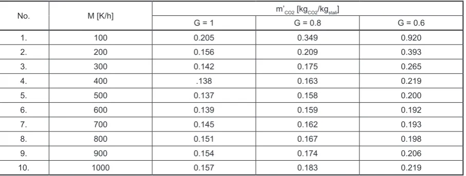
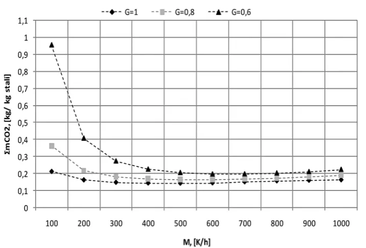
When analyzing the calculation results it can be noticed that with the increase in steel loss, with the corresponding increase in heat consumption, carbon dioxide emission increases. The values of CO₂ emission through the loss of steel are much lower than those resulting from heat consumption. The calculation results presented in Table 3 indicate that the value of CO₂ emission at heat-ing rates of M = 600–1000 K/h are nearly identi -cal for each of the heating technologies. Only for the initial heating rates the difference between the heating conducted at the constant surface temper-ature increase rate (G = 1) and the curvilinear sur -face temperature variation (G = 0.6) can be seen. The total carbon dioxide emission, as depend-ent on the heating rate, for the technologies under analysis is represented in Figure 2.

Table 1. Results of the calculation of the effect of heating rate on the emission of CO2 for different heating

tech-nologies, depending on the heat consumption magnitudes

No. M [K/h] m’CO2 [kgCO2/kgstali]

G = 1 G = 0.8 G = 0.6

1. 100 0.205 0.349 0.920

2. 200 0.156 0.209 0.393

3. 300 0.142 0.175 0.265

4. 400 .138 0.163 0.219

5. 500 0.137 0.158 0.200

6. 600 0.139 0.159 0.192

7. 700 0.145 0.162 0.193

8. 800 0.151 0.167 0.198

9. 900 0.154 0.174 0.206

10. 1000 0.157 0.183 0.219

Table 2. Results of the calculation of the effect of heating rate on the emission of CO2, depending on the steel loss

value for G = 1

No. M [K/h] z [kg/m2_] _z’_[kg/kg] _q’_[kJ/kg] _m”

CO2 [kgCO2/kgstali]

1. 100 4.396 0.0040 140.00 0.0076

2. 200 3.394 0.0031 108.50 0.0060

3. 300 3.183 0.0029 101.50 0.0056

4. 400 3.152 0.0028 98.00 0.0054

5. 500 3.171 0.0028 98.00 0.0054

6. 600 3.186 0.0028 98.00 0.0054

7. 700 3.227 0.0029 101.50 0.0056

8. 800 3.268 0.0029 101.50 0.0056

9. 900 3.292 0.0030 105.00 0.0058

(5)

21

Table 3. Results of the calculation of the effect of heating rate on the emission of CO2 for different heating

tech-nologies, depending on the steel loss value

Lp. M [K/h] m”CO2 [kgCO2/kgstali]

G = 1 G = 0.8 G = 0.6

1. 100 0.0076 0.0138 0.0361

2. 200 0.0060 0.0076 0.0151

3. 300 0.0056 0.0062 0.0091

4. 400 0.0054 0.0058 0.0070

5. 500 0.0054 0.0056 0.0062

6. 600 0.0054 0.0054 0.0056

7. 700 0.0056 0.0054 0.0054

8. 800 0.0056 0.0056 0.0054

9. 900 0.0058 0.0056 0.0056

10. 1000 0.0058 0.0058 0.0056

When examining the results represented in Figure 2 it can be found that depending on the method of operation of heating equipment, at rational heating rates and through the selec-tion of the heating technology, the carbon di-oxide emission can be substantially reduced. The calculation results indicate that, from the point of view of both ecological and economic assessment, it is disadvantageous to heat steel charge at loss heating rates (low furnace ca-pacities), as this will result in a considerable increase in CO₂ emission. The lowest CO₂ emission indices were achieved for heating conducted at a constant surface temperature increase rate (G = 1).

Fig. 2. Effect of the heating rate on the total CO2 emission for selected technologies

SUMMARY

From the performed numerical computations and the analysis of the obtained results, the fol-lowing conclusions can be drawn:

1. The results of numerical modelling show that for each heating case there is a specific heating rate that assures the minimum heat consump-tion, steel loss and CO₂ emission.

2. The carbon dioxide emission level is directly related to the unit heat consumption index and, indirectly, to the loss of steel.

(6)

Advances in Science and Technology Research Journal Vol. 9 (27) 2015 4. The reduction of carbon dioxide emission

can be achieved by using rational heating rates (M = 500–600 K/h).

5. The lowest CO₂ emission level is assured by charge heating conducted at a constant surface temperature increase rate, i.e. by using the technology G = 1.

REFERENCES

1. Kieloch M.: Energooszczędne i małozorzelinowe nagrzewanie wsadu stalowego. Częstochowa, Wydawnictwo WIPMiFS Politechniki Często-chowskiej, 2002.

2. Kieloch M.: Racjonalizacja nagrzewania wsadu. Częstochowa, Wydawnictwo WIPMiFS Politech-niki Częstochowskiej, 2010.

3. Kieloch M., Boryca J.: Analysis of influence of the speed of growth of temperature surface of steel charge on CO2 emission. The Holistic Approach to Environment 1, 2011, 19–27.

4. Kieloch M., Klos A., Warwas E., Boryca J.: Badania wpływu szybkości podgrzewania wsadu stalowego na emisję CO2. Hutnik-Wiadomości hutnicze, 5, 2009, 324–329.

5. Krajowy Plan Rozdziału Uprawnień do emisji dwutlenku węgla na lata 2008–2012 dla wspól-notowego systemu handlu uprawnieniemia do emisji, www.mos.gov.pl.

6. Musiał P., Burchart-Korol D.: Ograniczenie emisji CO₂ w przedsiębiorstwach hutniczych. Hutnik- Wiadomości Hutnicze, 10, 2008, 611–614.