University of New Orleans University of New Orleans
ScholarWorks@UNO
ScholarWorks@UNO
University of New Orleans Theses and
Dissertations Dissertations and Theses
1-20-2006
An R*-Tree Based Semi-Dynamic Clustering Method for the
An R*-Tree Based Semi-Dynamic Clustering Method for the
Efficient Processing of Spatial Join in a Shared-Nothing Parallel
Efficient Processing of Spatial Join in a Shared-Nothing Parallel
Database System
Database System
Gayatri Ganpaa
University of New Orleans
Follow this and additional works at: https://scholarworks.uno.edu/td
Recommended Citation Recommended Citation
Ganpaa, Gayatri, "An R*-Tree Based Semi-Dynamic Clustering Method for the Efficient Processing of Spatial Join in a Shared-Nothing Parallel Database System" (2006). University of New Orleans Theses and Dissertations. 298.
https://scholarworks.uno.edu/td/298
This Thesis is protected by copyright and/or related rights. It has been brought to you by ScholarWorks@UNO with permission from the rights-holder(s). You are free to use this Thesis in any way that is permitted by the copyright and related rights legislation that applies to your use. For other uses you need to obtain permission from the rights-holder(s) directly, unless additional rights are indicated by a Creative Commons license in the record and/or on the work itself.
AN R*-TREE BASED SEMI-DYNAMIC CLUSTERING METHOD
FOR THE EFFICIENT PROCESSING OF SPATIAL JOIN IN A
SHARED-NOTHING PARALLEL DATABASE SYSTEM
A Thesis
Submitted to the Graduate Faculty of the
University of New Orleans
in partial fulfillment of the
requirements for the degree of
Masters of Science
in
The Department of Computer Science
by
Gayatri Ganpaa
B.Tech, Jawaharlal Nehru Technological University, India, 2003
Acknowledgement
This thesis is the result of one and half years of work whereby I have been accompanied and assisted by many people. I have now the opportunity to express my gratitude to all of them. Instead of listing names after names, however, I will just say one big thanks to all the people who deserve to be thanked but not mentioned here by name.
I am highly indebted to my advisor, Professor Mahdi Abdelguerfi. He deserves my heartfelt appreciation for the warm and constant support he has given me to accomplish this thesis. In addition, I would like to thank Dr. Shengru Tu and Dr. Nauman Chaudhry for being on my thesis committee.
A special thanks goes to Mr. Venkata Mahadevan whose continuous support in getting this thesis prepared is invaluable. If it were not for his well-organized instruction, I would not imagine completing this successfully.
Table of Contents
List of Figures ... vi
List of Tables ... viii
Abstract... ix
1. Introduction...1
2. Overview of Parallel Spatial Databases and Survey of Previous Work ...3
2.1 Overview of Spatial Databases ...3
2.1.1 Spatial Databases ...3
2.1.2 Spatial SQL...4
2.1.3 Spatial Databases ...4
2.1.4 Types of Spatial Queries...5
2.1.5 Spatial Indexing ...6
2.2 Parallel Databases ...10
2.2.1 Why Parallel Spatial Databases ...10
2.2.2 How it works...10
2.3 Survey of Declustering Algorithms and Join Algorithms...11
2.3.1 Survey of Declustering Algorithms ...11
2.3.2 Survey of Join Algorithms ...13
3. Hardware and Software Tools Used ...15
3.1 Beowulf Cluster ...15
3.2 Spatial Databases: PostgreSQL/ PostGIS ...18
3.3 Programming Environment...19
3.4 Datasets used for Testing ...20
4. Methodology...24
4.1 Diag. Representation of the Parallel Processing of Spatial data...24
4.2 Declustering ...26
4.3 Parallel Execution of the Query...29
4.4 Viewing...31
4.5 User Interface...33
5. Discussion of Algorithms ...37
5.1 Spatial Declustering Techniques...38
5.1.1 Tiling technique (Declustering Using Replication) ...39
5.1.1.1Declustering Algorithm using the Tiling technique ...39
5.1.1.2Implementation Details...42
5.1.2 R*-tree semi-dynamic approach ...43
5.1.2.1Declustering Algorithm using the R*-tree semi- dynamic approach ...44
5.1.2.2Implementation Details...45
5.2 Spatial Joins ...50
5.2.2 Spatial Join in Parallel ...51
5.3 Join Algorithms...55
5.3.1 Join Algorithms for Tiling Technique ...55
5.3.1.1Clone Join Algorithm, Variant 1(CJAV1) ...56
5.3.1.2Clone Join Algorithm, Variant 2(CJAV2) ...57
5.3.2 Join Algorithm based on R*-tree Semi-Dynamic Approach...60
5.4 Rendering……….61
5.4.1 Rendering a Shapefile……… 63
5.4.2 Rendering from PostGIS………64
5.4.3 Viewer………64
6. Results & Discussion of Results………...66
6.1 Tiling Scheme……….. 66
6.1.1 Results on Declustering………. 66
6.1.2 Results of Join Algorithm for Tiling Scheme……… 71
6.1.2.1Variation of the Number of Tiles……….72
6.1.2.2Variation of the Number of Nodes…………...73
6.1.2.3Comparison of the Two Clone Join Algorithms………... 77
6.2 R*-tree based Semi-Dynamic Approach ……… 78
6.2.1 Declustering Results of a single relation………... 78
6.2.2 Declustering Results of two relations for a Join………… 79
6.3 Comparison of the Declustering techniques……… 85
6.3.1 Comparison of the Declustering Times………. 85
6.3.2 Comparison of the Join Results………. 86
7. Conclusion & Future work………...89
References………...90
List of Figures
Figure 2.1 Example of a R-tree...9
Figure 3.1 Overview of 72-node Beowulf Cluster...16
Figure 3.2a Hydro Dataset of a collection of States ...22
Figure 3.2b Rail Dataset of a collection of States...22
Figure 3.3a Hydro Dataset of Louisiana ...23
Figure 3.3b Rail Dataset of Louisiana ...23
Figure 4.1 Parallel Processing of Spatial Data...26
Figure 4.2 Declustering...29
Figure 4.3 Parallel Execution of the Query ...30
Figure 4.4 Viewer ...32
Figure 4.5 Adding Layers from Shapefile ...32
Figure 4.6 Adding Layers from PostGIS ...33
Figure 4.7 User Interface ...35
Figure 4.8 Table Option in the Interface...36
Figure 5.1 Data Distribution Skew ...40
Figure 5.2 Declustering Tiling Technique ...41
Figure 5.3 R*-tree built on the first relation ...47
Figure 5.4 Declustering second relation based on the R*-tree structure of the first relation...48
Figure 5.5 Spatial Join Operation ...51
Figure 5.6 Parallel Spatial Join Operation ...51
Figure 5.7 Plane Sweep Algorithm for the Filter Step...53
Figure 5.8 Clone Join Algorithm, Variant 1 (CJAV1) ...57
Figure 5.9 Clone Join Algorithm, Variant 2(CJAV2) ...59
Figure 5.10 Join Algorithm based on Semi-Dynamic Approach...60
Figure 5.11 Difference between Join Algorithm based on Semi-Dynamic Approach and CJAV2 ...61
Figure 6.1 Co-efficient of Variation vs. tiles for the dataset1 ...68
Figure 6.2 Co-efficient of Variation vs. tiles for the dataset2 ...69
Figure 6.3 Replication vs. Tiles for the dataset1 ...70
Figure 6.4 Replication vs. Tiles for the dataset2 ...71
Figure 6.5a: Time vs. # of Tiles for the dataset1. CJAV2 using 16 nodes ...72
Figure 6.5b Time vs. # of Tiles for the dataset2. CJAV2 using 16 nodes ...72
Figure 6.6 Time (ms) vs. Nodes for the Dataset1 (3,600 tiles) ...74
Figure 6.7 Time (ms) vs. Nodes for the dataset2 (8,100 tiles) ...76
Figure 6.8 CV vs. M (R*-tree on hydrolin) using dataset1 ...78
Figure 6.9 CV vs. M (R*-tree on hydrolin) using dataset2 ...78
Figure 6.10 Replication vs. M (16 nodes) for dataset1...82
Figure 6.11 CV vs. M (16 nodes) for dataset1...82
Figure 6.12 Replication vs. M for R*-tree based Semi-Dynamic approach...83
List of Tables
Table 3.1 Louisiana TIGER Data Information ...21
Table 3.2 TIGER data of a collection of adjacent States (Louisiana, Kansas, Mississippi, Arkansas, Texas, Oklahoma, and Missouri) in the US...22
Table 5.1 Tiling Scheme Data Distribution ...42
Table 5.2: First Hash Function...48
Table 5.3: Second Hash Function ...49
Table 5.4 Replication Rate with the two hashing functions ...50
Table 6.1 Decluster Times of all the Variants for dataset1...85
Table 6.2 Decluster Times of all the Variants for dataset2...85
Table 6.3 Comparison of 2 variants of R*-tree based Semi-Dynamic approach with CJAV2 using dataset1...87
Abstract
The growing importance of geospatial databases has made it essential to perform
complex spatial queries efficiently. To achieve acceptable performance levels, database systems
have been increasingly required to make use of parallelism. The spatial join is a computationally
expensive operator. Efficient implementation of the join operator is, thus, desirable. The work
presented in this document attempts to improve the performance of spatial join queries by
distributing the data set across several nodes of a cluster and executing queries across these
nodes in parallel.
This document discusses a new parallel algorithm that implements the spatial join in an
efficient manner. This algorithm is compared to an existing parallel spatial-join algorithm, the
clone join. Both algorithms have been implemented on a Beowulf cluster and compared using
real datasets. An extensive experimental analysis reveals that the proposed algorithm exhibits
Chapter 1 Introduction
The use of geospatial data arises in many applications including Cartography, Computer
Aided Design (CAD), Computer Vision, and Robotics to name but a few. Geospatial data sets
are often large and are being constantly gathered by numerous satellites and other data collection
devices. In order for the data collected to be useful, it needs to be processed and analyzed. This
data is typically stored in a spatial database to facilitate processing and analysis. However, due
to the massive amount of data being stored, several problems can arise. The ability to store and
query this enormous amount of data is critical but may lead to performance degradation.
Therefore, faster data retrieval and computation mechanisms are now required.
Performance problems with large databases have been widely documented by researchers
and several techniques [3, 4, 13, 15, 16, 17, 18, 20, 23, 25] have been devised to cope with this.
Indeed, traditional database management architectures have difficulty meeting the I/O and
compute performance levels needed to handle large volumes of geospatial data. To achieve
acceptable performance levels, database systems have been increasingly required to make use of
Parallelism [8]. One form of parallelism involves the use of compute clusters.
A cluster is simply a collection of compute nodes interconnected via some sort of
network. Clusters can improve the performance of geospatial queries by exploiting parallelism.
The most popular type of compute clusters in use today is based on the Beowulf paradigm.
are called slave nodes, are isolated on a high-speed private network that is not directly visible to
the outside world. A single computer connected to the outside world (called the master node)
lets a user login to the cluster and submit jobs for processing i.e. by spawning processes that will
execute on the slave nodes. Beowulf clusters help speedup program execution time, which is
made possible by splitting a task into several sub-tasks that can run in parallel on the slave nodes.
As it pertains to database architectures, many schemes have been developed to distribute data
across several databases (nodes). Also, there are many algorithms that have been researched to
perform the Spatial Join operation. These schemes should theoretically improve the execution
time of geospatial queries by performing program tasks in parallel. Several schemes and their
implementation details are discussed in this document.
The work presented in this document attempts to improve the performance of spatial
queries by distributing the data set across several nodes of a cluster and executing queries across
these nodes in parallel (in particular, the work is aimed at reducing the time required for Spatial
Join Queries). The rest of this thesis is organized as follows. Chapter 2 provides an overview of
spatial databases and distributed spatial databases. Chapter 3 discusses the hardware used
(including the Beowulf cluster), software used, and the test data used. Chapter 4 describes the
entire process of distributing, querying and visualizing the spatial data; it also describes the user
interface developed for performing these operations. Chapter 5 discusses the various
declustering techniques, Join algorithms, and rendering operations. Chapter 6 describes the
experiments performed and also discusses the results. Chapter 7 concludes with suggestions for
Chapter 2 Overview of Parallel Spatial Databases & Survey of
Previous Work
This chapter reviews spatial databases and discusses the need for parallel spatial
databases. Also surveyed are various declustering algorithms and join algorithms. The first
section gives a brief overview of spatial databases, spatial data types, spatial queries, and spatial
indexing. The second section discusses the need for parallel spatial databases and describes the
methodology used to deploy parallel spatial databases. The third section surveys declustering
and join algorithms.
2.1 Overview of Spatial Databases
2.1.1 Spatial Database
A spatial database [11, 12] describes the location and shape of geographic features. A
spatial database system is a database system with additional capabilities for handling spatial data.
In particular, a spatial database system provides spatial data types in its data model and query
2.1.2 Spatial SQL
SQL is a standard query language for Relational DBMSs. In this case, it has been
extended with spatial types to create spatial SQL. Databases have also been extended to support
these new spatial data types. Current ORDBMSs support user defined data types, including
spatial types.
The Open GIS Consortium [21] was founded by various software vendors to formulate
industry-wide standards related to GIS interoperability. The OGIS standard recommends a set of
spatial data types and functions which are crucial for spatial data querying. In this work,
PostgreSQL/PostGIS is the spatial database system used. PostgreSQL [2] is an ORDBMS that is
extended to support spatial data types. PostGIS is an extension to PostgreSQL which allows GIS
(Geographic Information Systems) objects to be stored in the database. PostGIS also includes
support for GiST-based R-Tree spatial indexes, and functions for analysis and processing of GIS
objects. The GIS objects supported by PostGIS are a superset of the "Simple Features" defined
by the OpenGIS Consortium (OGC). The latest version of PostGIS supports all the objects and
functions specified in the OGC "Simple Features for SQL" specification [21].
2.1.3 Spatial Data Types
Point: Discrete location represented as a coordinate pair. For example, a city may be
represented as a point in a large geographic area. E.g.: (0 0)
LineString: Set of ordered coordinates represented by a string of coordinates. Examples could
be rail road tracks and streams. E.g.: (0 0, 1 1, 1 2)
Polygon: Closed feature whose boundary encloses a homogeneous area represented by a closed
string of coordinates which encompass an area. Examples could be land use areas and lakes.
E.g.: (0 0, 4 0, 4 4, 0 4, 0 0)
MultiLineString: Collection of Lines. E.g.: ((0 0, 1 1, 1 2), (2 3, 3 2, 5 4))
MultiPoint: Collection of Point Objects. E.g.: (0 0, 2 3)
MultiPolygon: Collection of a set of polygons. E.g.: (((0 0, 4 0, 4 4, 0 4, 0 0), (1 1, 2 1, 2 2, 1 2,
1 1)), ((-1 -1,-1 -2,-2 -2,-2 -1,-1 -1)))
GeometryCollection: Collection of different objects. E.g.: (POINT (2 3), LINESTRING ((2 3,
3 4)))
The objects in space have to be represented by a spatial database system. These could be
represented as any of the above data types. For example, the objects in space could be thought of
as cities, streams, buildings, etc.
2.1.4 Types of Spatial Queries
In general, spatial queries can be classified as single scan and multi scan queries:
1. Single Scan: Single scan queries usually necessitate a single scan through the relation
objects stored in the corresponding relation. Window & distance queries are examples of single
scan queries.
“Find all the features within a Bounding Box” is an example of a window query. For a
distance query, it is possible to express queries such as “return all features within 100 units of a
particular point”. The above queries in PostGIS are as follows:
Window Query: SELECT gid, the_geom FROM <table_name> WHERE the_geom
&& GeometryFromText (`BOX3D (X1 Y1, X2 Y2) `:: box3d, -1)
Distance Query: SELECT gid, the_geom FROM <table_name> WHERE distance
(the_geom, GeometryFromText (`POINT(X Y) `, -1)) < 100
The first query is a bounding box query – it specifies that all features that lie within the
specified bounding box should be returned. The second query specifies that the feature ids and
features that lie within 100 units from a given point should be returned.
2. Multi Scan: Multi scan queries involve instances where objects have to be accessed
several times. Therefore, execution time is generally not linear but super linear with respect to
the number of objects. For example, a spatial join operation in a relational database system is a
multi scan query. A spatial join is a join which compares any two objects through a predicate on
their spatial attribute values.
Consider two relations hydrolin and rail. Each of these relations has the geometry
a river” is an example of a spatial Join. In this example, we are using a spatial distance function
as the join condition.
Spatial Join: SELECT h.gid, r.gid FROM hydrolin as h, rail as r WHERE
distance (h.the_geom, r.the_geom) = 0
Again, consider two relations bc_roads and bc_municipality. The query “What is the
length of the roads contained within each municipality?” is an example of a spatial join. In this
example, a spatial interaction condition “contains” is used as the join condition.
Spatial Join: SELECT m.name, sum (length (r.the_geom))/1000 as roads_km
FROM bc_roads AS r, bc_municipality AS m WHERE overlaps
(r.the_geom, the_geom) AND contains (m.the_geom, r.the_geom)
GROUP BY m.name ORDER BY roads_km
The spatial join is a computationally intensive operator to implement. The efficient
implementation of the spatial join operator is, thus, desirable. Spatial Joins are usually
performed in two steps: Filter step & refinement step. In the filter step, an approximation of the
spatial object, for example the minimum bounding rectangle, is used to remove the features
which are not part of the result, and produce candidates that are a superset of the actual result. In
the refinement step, each candidate is examined to check if it is part of the result – this is a
CPU-intensive operation. This check requires running a CPU-CPU-intensive computational geometry
2.1.5 Spatial Indexing
Spatial indexing enables efficient access to the data. There are two major trends for
indexing spatial data. The first trend uses space-driven structures; these are indices based on
partitioning of the embedding 2D space into rectangular cells, independent of the distribution of
objects. The most popular space-driven structure is the Quadtree and its variants. The second
trend uses data-driven structures; these indices are based on partitioning the set of objects
independent of the space. Examples of data-driven structures are the tree and its variants.
R-trees are more popular than Quadtree’s. This is because unlike the Quadtree, an R-tree adapts to
data distribution while keeping the tree balanced. Therefore, the body of work focuses only on
the R-tree and its derivatives.
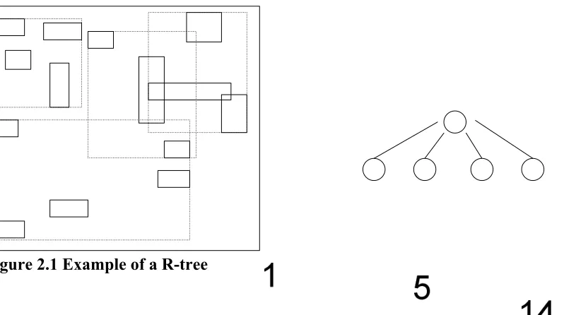
R-trees [26], introduced by Guttman, are an extension of the B-tree designed for efficient
indexing of multidimensional objects with spatial extent. An R-tree is a height balanced tree. A
leaf node contains an array of entries, [MBR, OID] where MBR is the Minimum Bounding
Rectangle of the object in the database and OID is the Object identifier. A non leaf node
contains an array of entries of the form [MBR, child pointer] where child pointer is the address
of a lower node in the R-tree and MBR covers all the MBRs in the lower node’s entries. An
example of a R-tree is shown in Figure 2.1.
Figure 2.1 Example of a R-tree
The insertion algorithm for an R-tree will place a new entry E in the leaf node whose
MBR needs the least enlargement to include E. During a node overflow, the split algorithm will
split the node that overflows into two nodes. Then, the algorithm selects two entries which are
the most distant ones. These entries are the first entries of two nodes. The remaining entries are
assigned using as the criterion the minimum area required to cover the new entry.
The R*-tree [5] was introduced by Beckmann. The insertion algorithm follows the nodes
in which the MBR has the minimum increase of overlap. The R*-tree’s split algorithm chooses a
split that results in a minimum overlap between the MBRs, whereas the R-trees’s split algorithm
chooses the split that results in the least enlargement of the MBRs. The reinsertion algorithm
increases storage utilization and improves the quality of the partition making it almost
independent of the sequence of insertions. The R*-tree method minimizes both the coverage (for
2.2 Parallel Spatial Databases
2.2.1 Why Parallel Spatial Databases
With the rapid increase in the availability of spatial data from a wide variety of sources
like satellite images, mapping agencies, etc., there is an increasing demand for systems that can
store and effectively manipulate such large spatial data sets. Spatial database systems are the
solution of choice. The ability to store and query this enormous amount of data is critical but
may lead to performance degradation. The performance problems associated with large
databases have been widely documented by researchers for many years and several techniques
have been devised to cope with this. One of the techniques that have gained popularity in recent
years is parallel processing of spatial database operations. Spatial database operations are often
time-consuming and can involve a large amount of data, so they can generally benefit from
parallel processing. Parallelism improves the response time of spatial queries. The design of
parallel database systems [13] often provides an impressive speedup when processing spatial
queries. Data partitioning allows parallel database systems to exploit the I/O bandwidth of
multiple disks by reading and writing them in parallel.
2.2.2 How it works
With parallel database systems, the assumption is that there are multiple CPUs and multiple
compute clusters are probably the best-known example of shared nothing machines in existence today.
Each node of the cluster has a processor and disk and each node also holds a database instance stored
on its local disk. The spatial data is declustered into fragments, which are then distributed to the
compute nodes. The process of data distribution across multiple disks is called declustering. This
multi-processor architecture is used for executing the query in parallel; spatial queries are ideally
suited for parallel execution. After declustering the data, any query issued through the master node
will be invoked on the slave nodes (in parallel) and these nodes will return the results of the query
back to the master node. This parallel technique of querying a spatial database will make the spatial
queries execute faster.
2.3 Survey of Declustering Algorithms and Join Algorithms
2.3.1 Survey of Declustering Algorithms
Parallel database systems employ partitioning strategies to distribute database relations
across multiple processing nodes. It has been shown in [13] that the data can be distributed using
round-robin, hash, and range partitioning schemes. There are many other methods proposed for
declustering data. J.M. Patel and D.J.DeWitt in [3] propose a tiling scheme to partition the data.
This scheme is the spatial analog of virtual processor round-robin partitioning for handling
skews in parallel joins which was proposed in [14]. The tiling scheme proposed splits the
universe (which is the MBR of all the spatial features in a relation) into tiles. Features in a tile
could be reduced by increasing the number of tiles. A similar method for declustering has been
proposed for redundancy based declustering of spatial objects in a parallel spatial database in
[15]. In [15], the number of tiles is always equal to the number of partitions. The data is
synthetically generated and uniformly distributed, so data skew is not considered at all. A
declustering algorithm based on tiles is proposed in [4], in which it creates partial spatial
surrogates (approximation of the spatial feature) when the spatial features overlaps tiles that are
mapped to multiple nodes. This scheme reduces the disk overhead. It has been shown in [16]
that a space filling Hilbert curve could be used for declustering Cartesian product files with
multiple attributes; this approach could be applied to distribute data across processors for queries
which involve only one attribute.
In [18], it has been seen that a good declustering could be achieved by using a variation
of the Hilbert based declustering method [16], as applied in the Hilbert packed R-trees [19]. In
this method, the data is sorted on the Hilbert values of the centers of their rectangles and then
packed into R-tree leaf nodes. These leaves are assigned to the nodes in a round-robin fashion.
In [17], declustering algorithms for parallel spatial Joins are proposed. Different declustering
schemes are proposed using R*-trees [5]. R*-trees are used to perform a spatial join in a
shared-disk environment. Two R*-trees are built on the two relations on which the Join is performed,
the leaves of the R*-tree are distributed, and different schemes decide when and on which nodes
the leaves are distributed.
In this work, a new Join Algorithm which uses tree declustering is proposed. The
proposed in [17], two R*-tree structures are used to decluster the join inputs. In [17], a spatial
Join is performed in a shared disk architecture; this is in contrast to our new Join algorithm
which is performed in a shared nothing architecture.
2.3.2 Survey of Join Algorithms
Various spatial join algorithms have been proposed for evaluating spatial joins. Most of
the algorithms proposed decluster the relations into a number of fragments. The join is then
performed by pair-wise joining of these small fragments. The declustering algorithms proposed
for parallel spatial join algorithms generally fall into two categories: dynamic partitioning
function & static partitioning function. A Dynamic partitioning function inserts spatial features
into a spatial index, like an R-tree and distributes the leaves of the spatial index to nodes. A
static partitioning function divides the space into regions and maps the regions to nodes. The
spatial join algorithm proposed in [3], uses a static partitioning function. The work in [20]
examined the data partitioning mechanism for parallel spatial joins, in which it uses a static
partitioning function as well. In [4], two declustering functions are employed, namely
declustering using replication and partial spatial surrogates (approximation of spatial features).
The authors designed two Join algorithms: shadow join and clone join. Shadow join uses only
the approximation of spatial features when declustering and clone join uses the exact spatial
features. The shadow join is similar to the parallel spatial Join in [20], except that in [20] the
MBR of the entire feature is used while declustering. Spatial join processing in [25] is based on
grid representation of spatial objects. In [25], spatial data is decomposed by superimposing a
transforms. The z-values are then used to perform the spatial join. In [23, 24], Seeded trees are
used to create an index and then perform a tree join algorithm. In [17], R*-trees are used to
Chapter 3 Hardware and Software Tools Used
This chapter describes the hardware and software tools used for the experiments
presented in this thesis. A detailed overview of the Beowulf cluster, programming environment,
and the spatial databases used is provided. In addition, the datasets used for testing are also
described.
3.1 Beowulf Cluster:
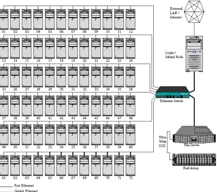
The vehicle utilized for parallel processing of spatial queries is a Beowulf cluster. The
Beowulf cluster housed at the Department of Computer Science at the University of New
Orleans consists of 72 compute nodes, 1 login/submit node, and 1 file server. 63 of the slave
nodes are 2.2 GHz Intel Pentium IV systems with 1 GB of memory, 20 GB of local disk storage,
and Fast Ethernet networking; the remaining 9 nodes are 2.4 GHz Intel Pentium IV systems with
1GB of memory, 20 GB of local disk storage, and Gigabit Ethernet networking. The file server
is a dual 1.4 GHz SMP Intel Xeon system with 2 GB of memory, 500 GB of disk storage, and
Gigabit Ethernet networking. Last, but not least, is the master node, which is a dual 2.2 GHz
SMP Intel Xeon system with 2 GB of memory, 300GB of disk storage, and 2 Ethernet interfaces.
The interface that links the cluster with the private Beowulf network is Gigabit Ethernet; the
external interface is 100BaseTX. All of the systems in the cluster are networked together by a
Cisco Catalyst 4000 series switch with 10/100/1000 auto-sensing ports and a 12-Gbps backplane.
This cluster was recently benchmarked using HPL 1.0, a portable, freely available
implementation of the standard High Performance Computing Linpack Benchmark. HPL solves
a random, dense linear system in double precision (64 bits) arithmetic on distributed memory
computers [9]. Benchmarking yielded a “theoretical peak” performance of approximately 63
Gigaflops. The amount of raw computing capacity provided is therefore quite substantial.
Figure 1 provides a broad overview of the cluster architecture.
There are 3 broad classes of parallel machines: shared memory systems, shared disk systems,
and shared nothing systems. In a shared nothing architecture, each processor has its own local
memory and disk − nothing is shared and all communication between the processors is
accomplished via the communication network. The shared nothing architecture is the most
widely used design for building systems to support high performance databases, primarily due to
its relatively low cost and flexible design.
Beowulf compute clusters are probably the best-known example of shared nothing
machines in existence today. A number of factors can be attributed to this including the
emergence of relatively inexpensive but powerful off-the-shelf desktop computers, fast
interconnect networks such as Fast Ethernet and Gigabit Ethernet, and the rise of the GNU/Linux
operating system. A compute cluster, for all intents and purposes, can be defined as a Pile of
Processors [7] interconnected via some sort of network. Each node in the cluster usually has its
own processor, memory, and optionally an I/O device such as a disk. However, it is important to
note that a cluster is not simply a network of workstations (NOWs) – in a cluster, the compute
nodes are delegated only for cluster usage and nodes typically have a dedicated, “cluster-only”
interconnect linking them. In the Beowulf paradigm, all of the compute nodes (also called slave
nodes) are isolated on a high-speed private network that is not directly visible to the outside
world. A single computer called the “master” or “head-end” provides a single entry point to the
cluster from the external network. This machine is sometimes referred to as the login or submit
node. Essentially, the master node is a system with 2 network interfaces – one connected to the
private Beowulf network and the other connected to the regular LAN. Users of the cluster will
on the slave nodes. Beowulf clusters are typically applicable to any area of research where a
speedup in program execution time is possible by splitting a large job into several sub-tasks that
can run concurrently on the compute nodes. This capability provides an intriguing setting for
evaluating the use of such a cluster for hosting large GIS databases, where there is an
ever-increasing need for greater computing power to process and query the massive amounts of
information being stored.
3.2 Spatial Databases: PostgreSQL/ PostGIS
PostgreSQL [2] is an object-relational database management system (ORDBMS) based
on POSTGRES, Version 4.2, developed at the University of California at Berkeley Computer
Science Department. PostgreSQL has a spatial extension called PostGIS that follows the
OpenGIS Consortium’s “Simple Features Specification for SQL” [21], a proposed specification
to define a standard SQL schema that supports storage, retrieval, query, and update of simple
geospatial feature collections via the ODBC API.
PostGIS [1] allows GIS (Geographic Information Systems) objects to be stored in a
PostgreSQL database and includes functions for analysis and processing of GIS objects. Point,
Line, Polygon, Multipoint, Multiline, MultiPolygon, and GeometryCollection object types can be
PostgreSQL is a good choice for use on a GNU/Linux system (such as our Beowulf
cluster) because of the robust, native support that it provides on this platform. Each of the nodes
in the Beowulf cluster executes the PostgreSQL server engine and has its own database instance
stored on its local disk; the file server is not used because of the potential performance penalty
associated with a large number of nodes accessing a shared file system simultaneously. Data
will instead be distributed evenly across the slave nodes and the user interface will be executed
on the master node. Any query issued through the master node will be invoked on the slave
nodes and the slave nodes will return the results of the query back to the master node.
3.3 Programming Environment:
The data visualization component has been programmed in Java using the Geotools [6]
Package, which is a leading open source Java library for developing OpenGIS [21] solutions and
has been in existence since 1996. As a result, Geotools has been used to develop the interface
for viewing geospatial data since it provides a rich set of graphics and rendering methods.
To decluster data across several nodes and to query the databases on all the nodes, Java
threads are used to make the queries run concurrently (in parallel) on the nodes. A Java program
is run on the master node, which creates threads to connect to the slave nodes, execute the
request, and get back the output to the master node. The PostgreSQL JDBC driver is used to
connect to the PostGIS database. JFreeChart [10] (a free Java library) is used to generate graphs
3.4 Datasets used for Testing:
Two collections of datasets were used for testing. Each collection has two datasets. The
first collection’s two geospatial data sets were obtained from the Bureau of Transportation
Statistics (BTS) [22]: the 2002 National Transportation Data Hydrographic and Railway network
Features of a collection of adjacent States (Louisiana, Kansas, Mississippi, Arkansas, Texas,
Oklahoma, and Missouri). Two datasets from the second collection were obtained from BTS as
well: the 2002 National Transportation Data Hydrographic Features of Louisiana State and the
2002 National Transportation Data Railway network of Louisiana State.
The Rail Network is a comprehensive database of the nation's railway system at the
1:100,000 scale. The hydrographic features are a state-by-state database of both important and
navigable water features. The Hydrography features include rivers, canals, etc. and the Rail
features represent railroads.
The first collection of datasets was for Louisiana State. The Hydrography dataset
contains data of Louisiana State. The spatial domain of this data set is west: 94.043189, East:
-88.758388, North: 33.019359 and South: 28.855127. The Rail dataset contains data of Louisiana
State as well. The spatial domain of this data set is west: -94.042735, East: -89.534031, North:
33.019180 and South: 29.376390. The second collection of datasets was for a collection of
adjacent states: Louisiana, Kansas, Mississippi, Arkansas, Texas, Oklahoma, and Missouri. The
40.613582and South: 25.837376. The spatial domain of the Rail dataset is west: -106.606615,
East: -88.111893, North: 40.590972and South: 25.891600.
These datasets are obtained as compressed ESRI Shapefile format. When imported into a
PostGIS database, the sizes of these datasets are given in Table 3.1 and Table 3.2.
Join queries are performed on each collection of datasets. The Join query joined the Rail
dataset with the Hydrography dataset. The query “find all the railways which are going across a
river” is a spatial join on Rail and Hydrography. Here, the spatial predicate is whether a railway
intersects a river.
When the Shapefiles are imported into PostGIS, each relation contains a feature-id, a few
columns describing the data, and the geometry itself. The feature type of the
feature-geometry may be one of 7 different types specified by the “Simple Features” specification of the
OpenGIS Consortium: point, linestring, polygon, multipoint, multilinestring, multipolygon, and
geometrycollection. The geometry of the features in these data sets is represented as type
MULTILINESTRING. This feature is represented in the database as a set of coordinates, which
may be either 2-dimensional or 3-dimensional. The features in these datasets are 2-dimensional.
Datasets # of features Total Size Type of Features
Hydrography 31400 20.1MB MULTILINESTRING
Rail 3543 1.8MB MULTILINESTRING
Datasets # of features Total Size Type of Features
Hydrography 99737 65MB MULTILINESTRING
Rail 35492 19MB MULTILINESTRING
Table 3.2 TIGER data of a collection of adjacent States (Louisiana, Kansas, Mississippi,
Arkansas, Texas, Oklahoma, and Missouri)in the US
The datasets are rendered and displayed in the following Figures: Figure 3.2.a and Figure
3.2.b display the hydrographic and railway data of a few states. Figure 3.3.a and Figure 3.3.b
display the data of Louisiana State.
Chapter 4 Methodology
This chapter describes the processes involved in the efficient parallel processing
of geospatial data. The different processes are declustering, querying, and visualization of
the spatial data. The user interface developed for visualization and the user interface that
was developed for executing commands across several nodes in parallel are also detailed
in this chapter.
The first section gives a pictorial representation of the process of declustering,
querying, and visualization of spatial data. This is followed by a description of each of
the processes in different sections. The last section deals with the user interface
developed for declustering the spatial data, and performing the parallel join operation.
4.1 Diagrammatic Representation of the Parallel Processing of Spatial
Data
The following are the main processes that are involved in performing a Join in
parallel. They are:
1. Declustering
2. Query Execution in Parallel
Declustering is the process of distributing data across several nodes. Query
Execution is done in parallel on the nodes. The results of the query are returned to the
master node, which merges the results to get the overall result for the query. The result
obtained from merging is visualized using a custom Geospatial Data Viewer.
A program runs on the master node which distributes data from the master node to
several slave nodes. After this preparation step, a query can be issued to the master node.
This query is then sent to all slave nodes i.e. the query execution is done in parallel across
the nodes. This design makes good use of the independent disk and memory subsystems
of each slave node. The results from the nodes are then sent back to the master node
which merges the result. The result of the query is visualized in the Viewer, a user
Figure 4.1 Parallel Processing of Spatial Data.
4.2 Declustering
Declustering is the process of distributing data across several nodes. A good
declustering technique distributes data such that,
1. There is nearly the same amount of data on each node (reduced data skew).
2. There is minimum replication of data on the nodes.
3. Parallel processing of a spatial join is done efficiently without the need for
The master node distributes data to several slave nodes. Each slave node has a
fragment of the data stored in its database. There are many distribution (partition)
techniques available. Some of them are basic round-robin, Tiling [3], Hilbert Curve [16],
Hilbert packed R-trees [18], Seeded Trees [23, 24] and Z-order [25] declustering
techniques.
The data is partitioned using a partitioning technique. A spatial partitioning
function divides both the join inputs into smaller partitions. The join is then performed by
pair wise joining of the smaller partitions. Spatial partitioning functions for spatial join
algorithms are usually categorized into two types: static and dynamic declustering
techniques.
In the static declustering technique, the space is initially decomposed into regions.
Each region is mapped to a disk and the features inside a region are stored on the disk the
region corresponds to. The tiling technique of [3] is an example of a static declustering
technique. In the dynamic declustering technique, the features are inserted into a spatial
index. The leaves of the spatial index are mapped to disks. In this method, the space is
decomposed into regions recursively. There are a minimum and maximum number of
features a region can have. Once a region exceeds the number of features than specified,
the region is split and the features are re-assigned to the two new regions. This process is
done recursively until all the features are inserted into a spatial index. In [17], a dynamic
declustering technique based on the R*-tree is proposed in a shared disk environment. It
the roots of both trees and traverses both trees in a depth first order. For each intersecting
pair of directory rectangles (minimum bounding rectangle of the data rectangles in the
corresponding subtrees), the algorithm follows the corresponding references to the nodes
in the lower level of the trees. Results are found when the leaf level is reached. The
leaves are then assigned to the disks by one of these mapping functions: a plane sweep
order, a round robin assignment or a dynamic assignment.
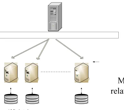
Figure 4.2 represents the declustering technique. The master node distributes data
using a declustering algorithm. After partitioning the data into fragments, a hashing
function is used to map the fragments to the nodes. In the case of the tiling scheme [3],
the data is divided into a set of tiles. Each tile is then mapped to a node by using a hash
function.
To distribute the data, the master node starts server socket programs on each of
the slave nodes. The role of this server socket is to receive data from the master node and
insert the data received into the database. Once the entire data set is distributed, the server
Figure 4.2 Declustering
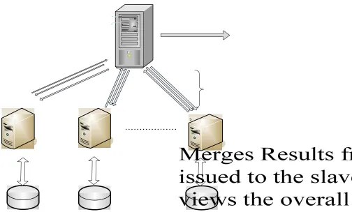
4.3 Parallel Execution of the Query
Each slave node has its own database instance. Once the data from the master
node is distributed, the query is executed. The query execution is done in parallel on each
The result of the query is sent back to the master
node.
Query is sent to the nodes
Merges Results from queries issued to the slave nodes
Master Node
Databases
Node 1 Node 2 Node n
Query issued to the master node
Network
Figure 4.3 Parallel Execution of the Query
The sequence of steps performed is as follows:
1. Query is issued at the master node.
2. The master node spawns several threads which connect to the slave nodes. Each
thread connects to a slave node and executes the query on the node. Each query is
3. After each query execution, each thread returns the result to the master node.
4. The master node merges the results from all the slave nodes and outputs the
overall result.
The result obtained is in textual format. However, the result obtained could also
be visualized in the Viewer, which is a user interface to view the spatial data. This is
explained in Section 4.4 below.
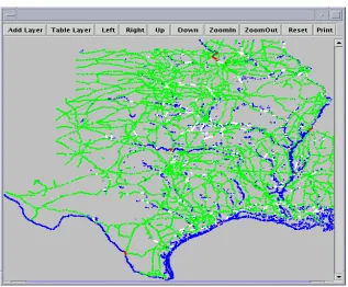
4.4 Viewing
The output from the execution of the query is in textual format. To view the
geographical output, the data is rendered in the viewer. The master node merges the
query results from all the slave nodes and renders the overall result in the developed
Viewer, pictured in Figure 4.4.
The viewer is a user interface developed for viewing spatial data. The Viewer
provides a number of tools to operate on the map. These tools are zooming, panning,
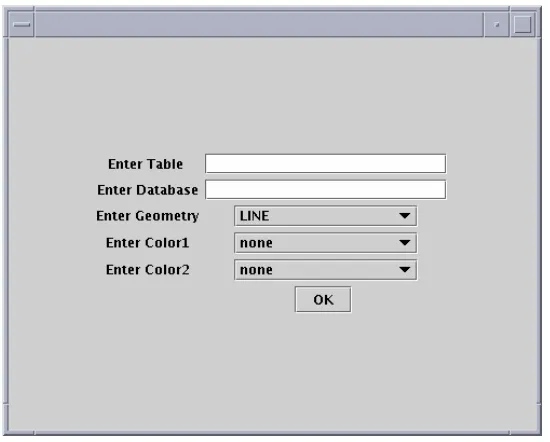
print, adding layers from Shapefiles and adding layers from PostGIS [1]. The Geotools
[6] library is used to build this interface. Figure 4.4 shows the viewer developed for
viewing the geospatial data. Figure 4.5 shows the adding layers from Shapefiles option in
Figure 4.4 Viewer
The algorithm to render a Shapefile is given in Section 5.4.1. The algorithm to
render data from PostGIS is given in Section 5.4.2. The form and the color of the
geometry are specified by the user (see Figure 4.5 & Figure 4.6).
Figure 4.6 Adding Layers from PostGIS
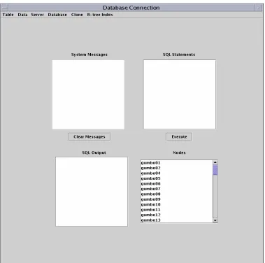
4.5 User Interface
The user interface provides for the loading of spatial data into the master node. It
also provides the capability for distributing, querying and updating of the spatial data to
multiple compute nodes in a cluster. The user interface enables the creation of tables and
databases before distributing the data to the nodes. This interface also lets the user send
commands to the nodes for execution. For example, to start a database server on all the
fragments of spatial data stored on the nodes. These algorithms are executed using this
interface.
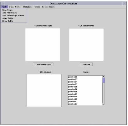
The User Interface developed for the above mentioned processes is seen in Figure
4.7. There are many options in the Menu bar: to create tables and databases, to start the
database server (PostgreSQL [2] server), to perform the parallel join algorithms, and to
decluster geospatial data. SQL queries, when given in the SQL Query Text Area in the
interface, can be executed on the nodes as needed. The number of nodes on which the
desired process is executed on is selected using this interface as well.
Figure 4.7 shows the interface developed. Figure 4.8 shows the Table option in
Chapter 5 Discussion of Algorithms
In [4], the two inputs to be joined are declustered using a static declustering
technique. The space is divided into a set of tiles and each tile is mapped to a disk. Each
of the two join relations is declustered using this technique. In [17], the join inputs are
declustered using a dynamic declustering technique. Two R*-tree structures are used to
decluster the data. The algorithm starts from the roots of both trees and traverses both of
the trees in a depth first order. For each intersecting pair of directory rectangles
(minimum bounding rectangle of the data rectangles in the corresponding subtrees), the
algorithm follows the corresponding references to the nodes in the lower level of the
trees. Results are found when the leaf level is reached. The leaves are then assigned to the
disks by either of these: a plane sweep order, a round robin assignment or a dynamic
assignment.
In this chapter, a parallel join algorithm based on a semi-dynamic declustering
technique is proposed. The proposed algorithm uses an R*-tree to decluster the first
relation. The second relation is declustered statically using a tiling like approach. The
leaves of the R*-tree, built on the first relation, is used to decluster the second relation.
The features of the second relation that intersect with a leaf are stored on the node that
The proposed algorithm is compared with two different versions of the clone join
algorithm proposed in [3]. It is noted that the clone join is a parallel join algorithm that
makes use of a static declustering technique based on tiling. The comparison of our
algorithm with the tiling based clone join is motivated by the well-established fact that
static declustering techniques perform better [20] than their dynamic counterparts.
The first section describes the spatial declustering techniques. Tiling scheme [3]
and the R*-tree based semi-dynamic approach are described. Implementation details of
these techniques are also provided. The second section reviews parallel spatial joins in
general. The third section discusses the join algorithms used. The fourth section describes
how the Geotools classes were used to render Shapefiles and data from the PostGIS
databases. This section also highlights the other features of the viewer.
5.1 Spatial Declustering Techniques
Two different techniques are implemented. The first one is the tiling technique
described in [4]. The second one is the proposed semi-dynamic approach which uses a
5.1.1 Tiling Technique (Declustering using Replication)
The tiling technique implemented in this chapter was originally proposed by Patel
& DeWitt in [4]. This technique is implemented to compare it with the new algorithm
presented in this work.
5.1.1.1 Declustering Algorithm using the Tiling technique
The universe of a relation is defined as the Minimum Bounding Rectangle that
covers all the spatial attributes of the relation. The universe of the relation to be
distributed is divided into a number of tiles of the same size. Each tile is mapped to a
node according to some hash function; to test this algorithm, a round robin function is
used. Spatial objects that are within a tile are stored on the node it is mapped to. Spatial
objects which overlap multiple tiles are stored on the nodes that correspond to these tiles.
So, the spatial objects that are within the first tile would be stored on the node it
corresponds to, and the objects that are within second tile will be stored on the node it is
mapped to and so on. If a spatial object overlaps more than one tile, it is stored in both
the nodes that map to these tiles. The number of tiles chosen should be no less than the
number of nodes.
This scheme presents two disadvantages, namely:
1. Data distribution skew
Data fragments stored on the various nodes may vary greatly in size, resulting in data
distribution skew. Also, because a spatial object could be stored on more than one node,
this results in replication of the same object.
The universe is a rectangle that covers all the features in a relation. It may
contain some regions where there are very few features. So, if the universe is divided into
a smaller number of tiles, then more data may be inserted on a node compared to the
other nodes as shown in Figure 5.1. One solution is to decrease the inequalities between
the nodes by increasing the number of tiles. As the number of tiles increases, the data
distribution skew reduces. However, because the universe is divided into more tiles,
many features may overlap more than one tile resulting in increased replication. Spatial
objects, which overlap more than one tile, are replicated in many nodes. So, when the
number of tiles increases, the percentage of replication grows.
Figure 5.1 Data Distribution Skew
Node 0 Node1
Node 2 Node 3
The universe is divided into tiles i.e., it’s divided into a number of rows and
columns. A hash function is usually utilized to map tiles onto nodes. An example of a
hash function is round robin. Given c columns and n compute nodes, a round robin
function will map the tile with the column number i and row number j onto node (i+j*c)
mod n.
The example of Figure 5.2 assumes 5 nodes and the universe composed of 16
tiles. A relation is being declustered across 5 nodes using 16 tiles. In the Figure, 1, 2, 3, 4
& 5 are the first 5 features of the relation. Feature 1 is stored on both Node 0 and Node1.
Feature 2 is also stored on both Node 0 and Node1. Feature 3 is stored on Node 2.
Feature 4 is stored on Node 0, Node 1, Node 3, and Node 4. Feature 5 is stored on Node
3.
3 1
4 2
5
Node 0
Node 1
Node 2
Node 3
Figure 5.2 Declustering Tiling Technique.
As it can be seen from Figure 5.2, there is both data replication and data
distribution skew. Feature 4 is stored on Nodes 0, 3 & 4. Also Feature 1 is stored on
Node 0 and Node 1, which shows a feature is replicated on more than one node. Also,
Node 0 has three features whereas Node 2 has just one feature which shows Data
Distribution Skew. This is listed in Table 5.1.
Nodes Features
0 1,2,4
1 1,2
2 3
3 4,5
4 4
Table 5.1 Tiling Scheme Data Distribution
5.1.1.2 Implementation Details
Using PostGIS [1] && (Overlaps operator) and the PostGIS [1] extent function,
returns true. The extent function takes a geometry column as an argument and will return
a BOX3D giving the maximum extend of all features in the table. The above mentioned
algorithm is implemented as follows:
• Get the universe of the table to be distributed using the extent function in PostGIS
[1]. Then use the xmin (Box3D), ymin (Box3D), xmax (Box3D) and ymax
(Box3D) functions in PostGIS [1] which gives xmin, ymin xmax, ymax points.
• Given these points, the universe (Minimum Bounding Rectangle of all features) is
divided into a number (# of rows * # of columns) of tiles.
• Make a Bounding Box, Box3D representation of each tile.
• For each bounding box use the && Overlaps operator in PostGIS [1] and get all
the spatial objects overlapping this bounding box and store the obtained
geometries in the node corresponding to that tile using the hash function described
above.
The above steps are performed for declustering one relation. For a spatial join,
two tables have to be declustered. This algorithm is used for spatial join because the same
algorithm could be applied to two different tables without any difficulties. In that case,
the universe should now be the Minimum Bounding Rectangle that covers all the spatial
features of both the relations.
This is a new algorithm proposed in this paper. The spatial data is declustered
using an R*-tree. The mapping of leaves to compute nodes is done via one of the two
hash functions we propose. Each of the two hash functions has its distinct advantages as
explained below.
5.1.2.1 Declustering algorithm using the R*-tree based Semi-Dynamic
approach
Using this algorithm, the problem of data replication and distribution skew are
reduced. An R*-tree [5] is built on the relation to be declustered. The R*-tree is an
indexing scheme for spatial data. The leaves of this tree are treated as tiles and are
distributed across various nodes. Each leaf of the R*-tree is mapped to a node according
to some hash function. The leaves of the tree are numbered from the left to the right.
There are two hash functions that have been used. The features within the leaves are
stored on the node the leaf is mapped to.
For the first hash function, k (where k = ┌Total leaves/ # of Nodes┐) successive
leaves are taken and are stored on each node. Consider an R*-tree built on a relation
which has total leaves as 21. The number of nodes the data has to be distributed onto is 3.
For the second hash function, each leaf is stored on a node in a round robin
fashion. For example, leaf number p is stored on the node p mod n, where n is the number
of nodes.
5.1.2.2 Implementation Details
The semi-dynamic R*-tree based declustering algorithm is implemented in Java.
xmin (feature), ymin (feature), xmax (feature) and ymax (feature) functions in PostGIS [1]
are used. These functions return the coordinates of the bounding box of the feature.
1. An external R*-tree is built on the relation to be distributed. The entries in this
R*-tree are the Minimum Bounding Rectangle (MBR) of the features in the
relation. To find the MBRs, the above mentioned functions of PostGIS are used.
2. Each leaf of the R*-tree is mapped to a node; the features that are inside a leaf are
located by querying the R*-tree for the entries in the leaf. These features are
inserted into the node the leaf corresponds to, which is determined by the hashing
function used.
The above mentioned approach is to decluster one relation. For a spatial join, two
relations have to be declustered using the R*-tree structure of usually the smallest
relation and is described below.
For the join algorithm, an R*-tree is built on one of the two relations (usually the
as described above for the first relation. The features of the second relation are distributed
statically using the tiling like approach. The leaves of the R*-tree built on the first
relation are assumed as tiles, and thus, the features of the second relation which overlap
the leaves are stored on the nodes corresponding to the leaves. Since the leaves of the
R*-tree do not overlap, there would not be any replication for the first relation, though there
would be some replication for the second relation. The second relation is not completely
declustered in this approach; only the features overlapping the leaves of the R*-tree
structure of the first relation are distributed since such features are only the candidates for
the Join.
The implementation details of the process of declustering the two relations for
spatial join are given below. To decluster two relations in this approach, the first relation
is declustered as explained in section 5.1.2.1, i.e. an R*-tree is built on it. So for every
leaf of the R*-tree of the first relation, the features that are within the leaf are stored on
the node the leaf correspond to. The features in the second relation which overlap this
leaf are stored on the same node.
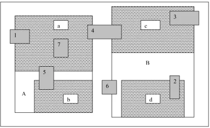
The examples of Figure 5.3 & Figure5.4 assume Relation 1 has 8 features (1, 2, 3
… 8), and Relation 2 has 7 features (1, 2, 3 …7). Figure 5.3 shows the R*-tree built on the
first relation: it has 4 leaves: a, b, c and d. It also shows the features numbered from 1
through 8. Each leaf is mapped to a node according to the hash functions as described
So for the first hash function, the features which are contained in leaves a and b
are stored on the first node. The features contained in the leaves c and d are stored on the
second node. For the second hash function, the features in leaves a and c are stored on the
first node and the features which are stored on leaves b and d are stored on the second
node.
The R*-tree structure of the first relation is used to decluster the second relation.
According to the first hash function, the features which overlap the leaves a and b are
stored on the first node and the features which overlap leaves c and d are stored on the
second node. For the second hash function, features which overlap a and c are stored on
first node and features which overlap b and d are stored on second node. Figure 5.4
illustrates the declustering for the second relation based on the R*-tree built on the first
relation.
4
7 5
2
3 1
8
6
a c
b d
A
Figure 5.3 R*-tree built on the first relation
Figure 5.4 Declustering Second Relation based on the R*-tree Structure of the First
Relation
As it is seen from Figures 5.4 & 5.5 above, the features of the two relations are
distributed among two nodes as shown in Tables 5.2 and 5.3.
Relation/ Node Node1 Node 2
Relation 1 1, 3, 6, 8 2, 4, 5, 7
Relation 2 1, 4, 5, 7 2, 3, 4
Feature
Leaves
1
5
4
7
3
2 6
a c
b d
A
Table 5.2 First Hash Function
Relation/Node Node 1 Node 2
Relation 1 1, 2, 3, 5 4, 6, 7, 8
Relation 2 1, 3, 4, 5, 7 2, 5
Table 5.3 Second Hash Function
It can be observed from Tables 5.2 & 5.3 that there is no replication for the first
relation, but there is replication for the second relation. Indeed for the second relation, in
Table 5.3, feature 5 is stored on both node 1 and node 2. Also for the second relation in
Table 5.2, feature 4 is stored on both the nodes.
The above two hashing methods each have advantages and disadvantages. With
the first one, if the answers of the spatial join request are concentrated geographically on
one part of the universe (say part A in Figure 5.3), then these answers will be computed
by only one node (node 1 in our example). This leads to data distribution skew. This
disadvantage is reduced with the second hashing function. The replication rate, using a
real dataset (see Chapter 6), of the second relation which uses the R*-tree of the first
relation is lower. But if the number of features a leaf can have is increased than the
replication rate with both the hash functions is almost the same.
Number of features (min/max) per leaf
10/20 35/70 100/200
Hashing func. 1 (range hash)
101.3 82.7 28.7
Hashing func 2 (round-robin)
200.4 99.8 25.6
Table 5.4 Replication Rate with the Two Hashing Functions.
5.2 Spatial Joins
5.2.1 Spatial Join Steps
Spatial joins typically operate in two steps, shown in Figure 5.5:
Filter Step: In this step, an approximation of each spatial object, the minimum bounding
rectangle is used to eliminate those tuples that cannot be part of the result; this produces a
set of candidate pairs for the spatial join.
Refinement Step: In this step, each candidate is examined to check if it part of the result;
Refinement Step Filter Step
Figure 5.5: Spatial Join Operation
5.2.2 Spatial Join in Parallel
For Spatial Join in parallel, the following steps are usually performed:
1. Declustering step
2. Filter & Refinement steps
The first step depends on the declustering algorithm used; both tiling as well as
R*- tree declustering are used. The declustering algorithms are explained in section 5.1.
Next, the filter and refinement steps are performed. Figure 5.6 shows the sequence of
steps.
Filter Step:
This step is performed on each node. A plane sweep algorithm [12] runs on each
node to perform this filter step: Let the two relations on which the join has to be
preformed be R and S. This step is performed on the MBR’s of the features. This step
eliminates the false hits, and gives the candidate pairs (the object identifier pairs (OID
pairs)). All the features of R and S are sorted in ascending order according to the x values
of their lower-left corners, xlof their MBR’s. The first feature in this set is picked; let it
be from the relation R, r. We now have to search in the sorted list S for all the rectangles,
looking for the ones whose lower x values, xl are smaller than the x values of upper-right
corner, xu of r, until an MBR in S is such that it has its xl value greater than the xu value
of r. The resulting pairs thus obtained are the ones which overlap with r along the x-axis.
These pairs are checked to see if they actually intersect, by checking to see if they
overlap along the y axis. If they do overlap then the pairs are added to the result of the
filter step. ‘r’ is marked as done and removed from the sorted set, and the processing
continues with the next element in the sorted set. A sweep line is assumed to move
though the sorted set. This process continues until one of the relations has been fully
Figure 5.7 gives a plane sweeping example. This example assumes there are 5
features in R, and 4 features in S. Let the features in R be {R1, R2, R3, R4, R5} and in S
be {S1, S2, S3, S4};
Y-axis
Figure 5.7 Plane Sweep Algorithm for the Filter Step
The entries are first sorted according to the xl values:
Sorted Set: {R2, R3, S1, S2, R1, S4, R4, S3, R5}
The process starts off with the first feature from the Sorted Set. In this case, R2 is
selected initially to begin the process: R2
R3
S1 S2
R4
S3 R5 S4
R1