Exploratory Toolkit for Evolutionary and Swarm-Based Optimization »

(1)

Exploratory Toolkit for

Evolutionary and Swarm-Based

Optimization

Namrata Khemka

Christian Jacob

Optimization of parameters or “systems” in general plays an ever-in-creasing role in mathematics, economics, engineering, and the life sciences. As a result, a wide variety of both traditional mathematical and nontraditional algorithmic approaches have been introduced to solve challenging and practically relevant optimization problems. Evolutionary optimization methods~in the form of genetic algorithms, genetic

pro-gramming, and evolution strategies~represent nontraditional

opti-mization algorithms that draw inspiration from the processes of natural evolution. Particle swarm optimization is another set of more recently developed algorithmic optimizers inspired by social behaviors of organisms such as birds [1] and social insects. These new evolutionary approaches in optimization are now entering the stage and are becoming very successful tools for solving real-world optimization problems [2]. We present Visplore

and Evolvica as a toolkit to investigate, explore, and visualize evolutionary and swarm-based optimization techniques. A webMathematica interface is also available.

‡

1. Introduction

(2)

The main focus of this article, however, is not on the optimization of parameters for the soccer kick model. Instead, we present what has been learned from our comparison studies of the evolution- and swarm-based optimizers on a set of selected benchmark functions. These benchmark studies turned out to be extremely useful in understanding the intricacies in performance regarding three optimizers: (1) the originally used H1+ lL ES; (2) a canonical (“basic”) PSO (bPSO); and (3) a PSO with noise-induced (“random”) inertia weight settings (rPSO). We describe and analyze the performance of each of these optimizers on five benchmark functions in two, four, and 10 dimensions. These findings are projected to performance characteristics that were found in the real-world appli-cation of the discussed soccer-kick model, which poses a 56-dimensional opti-mization problem. The Mathematica notebooks that were created provide us with insights regarding the relations between control parameters and system perfor-mance of the optimizers under study. Consequently, we gain a better under-standing of the algorithms on multidimensional real-world problems.

This article is organized as follows. In Section 2 we give descriptions of the three optimization algorithms used in our comparison. An introduction to the bench-mark functions and an outline of the experimental setup follows in Sections 3 and 4, respectively. We discuss the experimental results and summarize the lessons learned in Section 5. The accompanying webMathematica site is pre-sented in Section 6. The paper is concluded in Section 7.

‡

2. The Three Contenders

The three contenders for our comparative study of evolution- and swarm-based optimization algorithms are: (1) a relatively simple H1+ lL ES; (2) a canonical (“basic”) PSO (bPSO); and (3) a PSO with noise-induced (“random”) inertia weight settings (rPSO). The following subsections present these approaches in more detail.

· 2.1. (1+l) Evolution Strategy

ES has been a successful evolutionary technique for solving complex optimization problems since the 1960s [5]. ES evolves vectors of real numbers and the “genetic” information is interchanged between these vectors through recombination operators. Slight variations (“mutations”) on these vectors are obtained by evolving strategy parameters that determine the amount of change applied to each vector component.

In the H1+ lL ES scheme, a single parent is mutated l times. Each of the newly created offspring is evaluated, and the parents and the offspring are added to the selection pool. The single best individual among the 1+ l solutions in the pool survives and becomes the parent for the next iteration. Now we describe the

(3)

Hmêr + lL ES Algorithm

Ë Step 1. Initialize the population of size m by randomly assigning loca-tions P=Ip₁, … , p_i, … , p_mM and strategy parameters

S=I”s1, … ,”si, … ,”smM, where p_i=Ip_i₁, … , p_idMœd and

s ”

i=I”si1, … ,”sidMœd.

Ë Step 2. Using the recombination operator c, generate l ¥ m offspring by randomly selecting and recombining r individuals from the pool of m

parents.

• p_i£ _{= cI}_p

1£, … , pr£M, where pi£œP for 1§ j§ r.

• p_i£ ₌_IcI_p

11

£ _{, … ,} _p r1

£ _M_{, … ,} _cI_p

1d £ _{, … ,} _p

rd

£ _MM_{for 1}_§_k_{§ l}_.

• P£=Ip₁£_{, … ,} _p l£M. Ë Step 3. Mutations.

• p_k″ _:₌ _p k £₊_z”

k where z”k:=IN0ISk1M…N0ISkdMM for 1§k§ l.

• NaHSL returns a Gaussian distributed random value around a with

variance s.

• P″ ₌_P£₊_I_p

1

″_{, … ,} _p l″M.

Ë Step 4. Evaluate the fitness  of all individuals in P″_.

Ë Step 5. Select the m best individuals to serve as parents for the next generation.

• P=Best

m

@D HP″L.

Ë Step 6. If the termination criterion is met: • Stop.

• Otherwise, go to Step 2.

· 2.2. Basic Particle Swarm Optimization

As the bPSO we use the original PSO version introduced by Eberhart and Kennedy [6]. Inspired by both social behavior and bird flocking patterns, the par-ticles “fly” through the solution space and tend to land on better solutions.

The search is performed by a population of particles i; each has a location vector p_i =Ip_i₁, … , p_idMœd_{that represents a potential solution in a}_d_-dimensional

(4)

weight w was suggested by Shi and Eberhart [11, 12]. In the bPSO algorithm this term is set to the constant value w =1.

bPSO Algorithm

Ë Step 1. Initialize particle population of m particles by stochastically as-signing locations P=Ip₁, … , p_i, … , p_mM and velocities

V =In”1, … ,n”i, … ,n”mM.

Ë Step 2. Evaluate the fitness of all particles:

HPL=IHp₁L, … ,Hp_iL, … ,Hp_mLM.

Ë Step 3. Keep track of the locations where each individual had its highest fitness so far:

• Pbest ₌_J_p

1best, … , pibest, … , pmbestN where

p_ibest ₌ _p

i

new_{if and only if}__H_p

inewL>HpiL.

Ë Step 4. Keep track of the position with the global best fitness:

• p_globalbest ₌_max_ _I_Pbest_M_.

Ë Step 5. Modify the particle velocities based on the previous best and global best positions:

• n”inew= w n”i+ j1Jp_ibest-p_iN+ j2Jp_globalbest -p_iN for 1§i§n.

Ë Step 6. Update the particle locations:

• p_i =p_i+ n”inew for 1§i§n.

Ë Step 7. If the termination criterion is met: • Stop.

• Otherwise, go to Step 2.

· 2.3. Random Particle Swarm Optimization

Previous work with PSOs suggests that the so-called inertia weight w should be annealed (dPSO) over time in order to obtain better results [13]. This time-decreasing inertia weight facilitates a global search at the beginning and the later small inertia weight fine-tunes the search space. Since the annealed value is dependent on time, the number of iterations must be known in advance. However, in most real-world scenarios, like the soccer-kick optimization [2], it is extremely difficult to know the number of necessary iteration steps in advance. The “random” rPSO version tries to alleviate this problem by assigning a random number to w (Step 5) in each iteration as follows:

w = 0.5 +r

(5)

When r is a uniformly distributed random number in the interval @0, 1D, w is a uniformly distributed random number in the interval B1

4, 3 4F.

‡

3. Benchmarks

According to the no free lunch theorem [14], it is difficult to identify a clearly superior search or optimization algorithm in any comparison. Therefore our purpose is not to show which one of the three algorithms outperforms the others in any particular case, but to find out which of these optimizers is better suited for specific optimization challenges. In particular, we also want to investigate whether an algorithm’s performance characteristics in two dimensions~where visualization and manual inspection are easiest and most accessible~transfer to higher dimensions. We evaluate the performance of the H1+ lL ES scheme and both versions of the particle swarm algorithms on a small set of numerical benchmark functions.

We use the five benchmark functions illustrated and described in more detail fol-lowing. We explore each of these benchmark search spaces for dimensions d=2, d=4, and d=10. The first three functions are unimodal, that is, with a single global optimum. The last two functions are multimodal, where the number of lo-cal maxima increases exponentially with the problem size [15]. In the following function descriptions, x* denotes the location of the global optimum. In the func-tion plots, the locafunc-tion of the global optimum is marked by a red sphere.

Ë f1: Sphere

f1= -‚

j=1

d

x2j, -5.12§xj§5.12, Hx*L =0.

This is a simple, symmetric, smooth, unimodal search space (inverted parabola) and is known to be easily solved by all algorithms. As in our case, it is mainly used to calibrate optimizer control parameters.

-5 -2.5 0 2.5 5 x -5 -2.5 0 2.5 5 y -5 -2.5 0 2.5 5 x

Ë f2: Edge

f2= - ‚

j=1

d

°xj•+ ‰ j=1

d

(6)

The function f2 has shared edges, making it more difficult to find good so-

lutions around the ridges.

-10 -5 0 5 10 x _-10 -5 0 5 10 y -10 -5 0 5 10 x

Ë f3: Step

f3= - 12+‚

j=1

d

exju , -5.12§xj§5.12, Hx*L =0.

We included the linear surface function f3 in order to see whether the al-

gorithms perform a gradient ascent strategy.

-5 -2.5 0 2.5 5 x -5 -2.5 0 2.5 5 y -5 -2.5 0 2.5 5 x

Ë f4: Ackley

f4= - -20e -0.2 1

d⁄j=1

d _x j2

-e

1

d⁄dj=1cosI2pxjM₊₂₀₊_e _, _-₃₀_§_x

j§30, Hx*L =0.

(7)

Ë f₅: Griewangk

f₅= - 1+ 1

4000 ‚_j₌_i

d

x2_j-‰

j=1

d

cos xj j

, -100§xj§100, Hx*L =0.

Griewangk’s function has hundreds of local optima in the center. We included it to compare the algorithms’ performances on Griewangk and the sphere function.

-100 -50

0 50

100

x -100

-50 0

50 100

y

-100 -50

0 50

100

x

‡

4. Experimental Setup

For each of the three optimizers ES, bPSO, and rPSO, we performed 20 experi-ments on each of the five test functions f1 to f5 for dimensions d=2, d=4, and d=10. A different random number seed is used for each of the 20 runs. The ini-tial individuals (including those for ES) are uniformly distributed throughout the search space. Each initial population generated for an ES experiment is also used for the bPSO and rPSO experiments. This ensures that all comparable runs start with the same initial distribution of individuals. The termination criterion for all runs was to stop when the maximum number of iterations tmax=1500 was

reached. By that time all the optimizers had already reached their convergence phase (see Figure 2 later). The parameter settings for the three algorithms are de-scribed in Tables 1, 2, and 3.

Population size, n 10

Location range, pi j œAplow, phighE varies

Velocity range, vi j œAvlow,vhighE 10% ofpi j

Exploitation rate, j1 0.1

Exploration rate, j₂ 1

(8)

Population size, n 10 Location range, pi j œAplow, phighE varies

Velocity range, vi j œAvlow,vhighE 10% ofpi j

Exploitation rate, j1 1.5

Exploration rate, j2 1.5

Table 2. rPSO parameter settings.

Population sizeHselection poolL, 1+ l 1+9 Mutation step size radius 1

Table 3. ES parameter settings.

‡

5. Discussion of the Results

The results of the evolution-based optimizer and the two particle swarm optimi-zation techniques are briefly discussed in this section.

· 5.1. Phenotype Plots

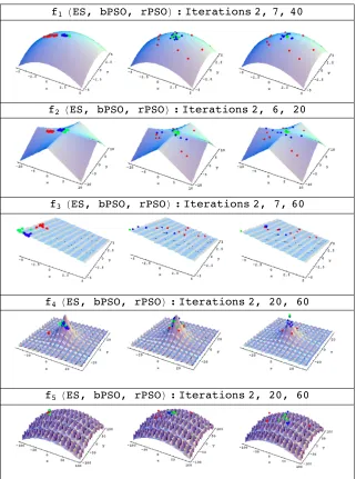
Figure 1 gives an example of the population dynamics resulting from each of the three algorithms (ES in column 1, bPSO in column 2, and rPSO in column 3) ap-plied over a certain number of iterations. The individuals are represented as dots where in each plot three iterations (red, blue, green) are depicted. In order to achieve a fair comparison, all three algorithms start from the same initial popula-tions. The behavior of the individuals is seen at different iterations, making it easy to compare and contrast the movement of the individuals and study their convergence behavior. For example, f1 is plotted at iterations 2 (red), 7 (blue),

and 40 (green).

In comparison to the H1+ lL ES scheme, we observe that the particle swarm indi-viduals (both bPSO and rPSO) have higher exploration capabilities, search the solution space more thoroughly, and search in multiple directions. The ES indi-viduals stay close to each other within a certain mutation radius. This is a typical effect of using this particular ES scheme. The individuals of the ES algorithm con verge to a local optimum solution for functions f4and f5. This also illustrates the

(9)

f1HES, bPSO, rPSOL: Iterations 2, 7, 40

(10)

· 5.2. Convergence Plots

The convergence plots represent mean fitness values computed over all 20 runs for all 1500 iterations. This graph helps to demonstrate the convergence behav-ior of the individuals of a particular algorithm and also illustrates which of the three algorithms has the fastest fitness convergence speed. Figure 2 summarizes the results, which are shown for d=2 (column 1), d=4 (column 2),and d=10 (column 3).

f1HES, bPSO, rPSOL: dimensionsH2, 4, 10L

(11)

In almost all cases, the ES algorithm is comparable to rPSO. The bPSO algo-rithm turns out to be the slowest in terms of convergence speed for d=2. How-ever, as the number of dimensions increases (d=4), the convergence rate of ES decreases, and in 10 dimensions ES converges more slowly and toward lower fit-ness values.

All three algorithms show relatively steep ascents during the first 100 or 200 iterations. In general, rPSO tends to rapidly level off without making any further progress (for most of the test cases) during the rest of the simulation; that is, the swarm stagnates and no changes are observed in terms of finding a better fitness value. For instance, on f1, particle swarms stagnate and flatten out without any

further improvements. However, the convergence rate of ES on the function f3

gradually slows down but does not completely level off, which indicates that if it is allowed to run longer it may discover better solutions.

Another observation made for function f₅ in two dimensions is that rPSO has the slowest convergence rate. This is in line with the results of the phenotype plot (Figure 1), where the particles do not converge to one location.

· 5.3. Success Plots

The best fitness value obtained at the end of each run is illustrated in Figure 3. For each function the fitness values of all 20 runs are plotted in ascending order from left to right. Therefore, each graph displays the success rate of each algo-rithm on a particular function. The best (right-most point), worst (left-most point), and mean fitness can also be easily derived from these graphs.

In all 20 runs, the ES algorithm finds worse solutions than both PSO algorithms for d=2, 4, and 10, as shown by the left-most blue point in Figure 3. This is in line with the results of the phenotype plots (Figure 1), especially for the multi-modal functions f4 and f5, where the ES individuals are unsuccessful in finding

the global optimum. The higher exploration capabilities of the PSO algorithms seem to facilitate the discovery of better solutions in comparison to the local ES scheme.

(12)

Figure 3. Success ratio plots of the benchmark functions f1 to f5. From left to right the columns show the best fitness value obtained at the end of each run of the three algo-rithms (ES: blue, rPSO: orange, bPSO: green) in 2, 4, and 10 dimensions.

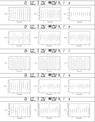
· 5.4. Parameter Range Plots

(13)

provide insights on whether the fitness function is sensitive with respect to a par-ticular variable or not. Figure 4 also clearly visualizes the stage of convergence in each dimension.

Figure 4 shows that the ES algorithm maintains a high parameter range in comparison to the particle swarm algorithms. This is in line with the results of Figure 2, where ES has the slowest convergence speed for d=10. Evolution strategies seem to consistently keep wider parameter ranges. Both particle swarm algorithms show comparable ranges.

f1HES, bPSO, rPSOL:t ¥ -5

(14)

‡

6. “Evolutionary Swarms” web

Mathematica

Site

The comparisons conducted provide knowledge and insights about the algo-rithms, while illustrating the movement of the individuals in the solution space (Figure 1). They point out various characteristics such as the convergence speed and the success an algorithm has in finding good solutions. The strengths and weaknesses of the algorithms are exploited. For example, PSO algorithms have a higher exploration rate, whereas the H1+ lL scheme of ES depicts a local search scheme.

We created a set of notebooks to compare the H1+ lL scheme of ES and both of the particle swarm optimizers on the benchmark functions (f1 to f5). We then

converted those notebooks to webMathematica. This interactive site provides a hands-on tutorial and an experimental environment through a selection of 10 benchmark functions along with visualization tools.

This site currently includes three variants of particle swarms: basic (bPSO), ran-dom (rPSO), and those with decreasing inertia weight (dPSO). We also imple-mented both of the simple ES schemes: the H1+ lL scheme and the H1, lL scheme as well as the generalized evolution strategies Hm + lL and Hm, lL as described in Section 2.

As it is in general difficult to know the settings of various parameters, we provide suggestions for different settings. This will help users to gain further knowledge regarding these optimizers.

The website can be accessed at www.swarm-design.org.

‡

7. Conclusion

The best way to understand and use evolution- and swarm-based algorithm heuristics is through practical experience, which can be gained most efficiently on smaller-scale problems. The Evolutionary & Swarm Optimization website that we developed will be merged with the collection of notebooks from the Evolvica package [16]. This database of notebooks and the swarm algorithms pro-vides an experimental and inquiry platform for introducing evolutionary and swarm-based optimization techniques to those who wish to further their knowl-edge of evolutionary computation. Making these notebooks available through a webMathematica site means that anyone with access to the newly built web pages will have instant access to a wide range of optimization algorithms.

‡

References

[1] C. Jacob and N. Khemka, “Particle Swarm Optimization: An Exploration Kit for Evolution-ary Optimization,” in New Ideas in Symbolic Computation: Proceedings of the Sixth In-ternational Mathematica Symposium (IMS’04), Banff, Alberta, Canada (P. Mitic, C. Jacob, and J. Carne, eds.), Hampshire, UK: Positive Corporation Ltd., 2004.

library.wolfram.com/infocenter/Conferences/6039.

(15)

[3] D. Goldberg, Genetic Algorithms in Search, Optimization, and Machine Learning, Read-ing, MA: Addison-Wesley Publishing Company, 1989.

[4] J. R. Koza, Genetic Programming: On the Programming of Computers by Means of Natu-ral Selection, Cambridge, MA: MIT Press, 1992.

[5] I. Rechenberg, “Evolution Strategies: Nature’s Way of Optimization,” Optimization Methods and Applications, Possibilities and Limitations (H. W. Bergmann, ed.), Lecture Notes in Computer Science, 47, Berlin: Springer, 1989 pp. 106|126.

[6] J. Kennedy and R. C. Eberhart, “Particle Swarm Optimization,” in Proceedings of the IEEE International Conference on Neural Networks, Perth, WA, Australia, New York: IEEE, 1995 pp. 1942|1948.

[7] G. Cole and K. Gerristen, Influence of Mass Distribution in the Shoe and Plate Stiffness on Ball Velocity During a Soccer Kick, Herzogenaurach, Germany: Adidas-Salomon AG, 2002.

[8] G. Cole and K. Gerristen, Optimal Mass Distribution and Plate Stiffness of Football Shoes, Herzogenaurach, Germany: Adidas-Salomon AG, 2002.

[9] G. Cole and K. Gerristen, Influence of Medio-Lateral Mass Distribution in a Soccer Shoe on the Deflection of the Ankle and Subtabular Joints during Off-Centre Kicks, Herzoge-naurach, Germany: Adidas-Salomon AG, 2003.

[10] N. Khemka, “Comparing PSO and ES: Benchmarks and Applications,” M.Sc. Thesis, Uni-versity of Calgary, Calgary, Alberta, Canada, 2005.

[11] Y. Shi and R. C. Eberhart, “Parameter Selection in Particle Swarm Optimization,” in Ev-olutionary Programming VII: Proceedings of the Seventh International Conference on Evolutionary Programming, San Diego, CA (V. W. Porto, N. Saravanan, D. E. Waagen, and A. E. Eiben, eds.), Lecture Notes in Computer Science, 1447, London: Springer-Ver-lag, 1998 pp. 591|600.

[12] Y. Shi and R. C. Eberhart, “A Modified Particle Swarm Optimizer,” in Proceedings of the IEEE Congress on Evolutionary Computation (CEC’98), Anchorage, AK, New York: IEEE, 1998 pp. 69|73.

[13] R. C. Eberhart and Y. Shi, “Comparison between Genetic Algorithms and Particle Swarm Optimization,” in Evolutionary Programming VII: Proceedings of the Seventh Interna-tional Conference on Evolutionary Programming, San Diego, CA (V. W. Porto, N. Sara-vanan, D. E. Waagen, and A. E. Eiben, eds.), Lecture Notes in Computer Science, 1447, London: Springer-Verlag, 1998 pp. 611|616.

[14] D. H. Wolpert and W. G. Macready, “No Free Lunch Theorems for Search,” SFI Working Paper # 95-02-010, Santa Fe, NM: Santa Fe Institute, 1995.

[15] H-P. Schwefel, Evolution and Optimum Seeking, New York: John Wiley & Sons, 1995.

[16] C. Jacob, Illustrating Evolutionary Computation with Mathematica (The Morgan Kauf-mann Series in Artificial Intelligence), San Francisco, CA: Morgan KaufKauf-mann Publishers, 2001.

Namrata Khemka, and Christian Jacob, “Exploratory Toolkit for Evolutionary and

(16)

About the Authors

Namrata Khemka received her Ph.D. in computer science from the University of Calgary in 2009. She received her M.Sc. in 2005 and B.Sc. in 2003. Her interests lie in data visualiza-tion, optimization techniques, and swarm- and agent-based modeling.

Christian Jacob received his Ph.D. in computer science from the University of Erlangen-Nuremberg in Erlangen, Germany. He is currently an associate professor in the Department of Computer Science (Faculty of Science) and the Department of Biochemistry & Molecular Biology (Faculty of Medicine) at the University of Calgary. Jacob’s research interests are in evolutionary computing, emergent phenom-ena, and swarm intelligence, with applications in civil engineering, biological modeling, medical sciences, computational creativity, and art.

Namrata Khemka Christian Jacob

University of Calgary, Calgary, AB, Canada, T2N1N4 [email protected]