River Bifurcations

(1)

River Bifurcations

Walter Bertoldi

(2)

Year: 2004

Supervisor: Prof. Marco Tubino Cotutor: Guido Zolezzi

Università degli Studi di Trento

Trento, Italy

(3)

where we face it as free beings admiring,

asking and observing, there we enter the realm of Art and Science.

(4)

(5)

I’m grateful to my supervisor, prof. Marco Tubino, for the constant support during my PhD study and for the enthusiasm in the research that he has transmitted to me.

Thanks to Guido, for the scientific support and most of all for the friendship and for the sharing

of joy and trouble of the research world.

I wish also to thank prof. Peter Ashmore for the period I spent at UWO and all the ’Sunwapta

international group’ for the wonderful summer and the important experience I lived in Canada. A special thank to all the ’Bonuti group’, Gianluca, Gianluca, Giuliano, Ilaria, Marco, Marco,

Stefano, friends before colleagues, with whom I shared these years, and in particular to my flatmate

GianDuca and GianLinux.

I’m grateful to all the students I worked with: Guido, Kilian, Anita, Edi, Igor, Tommaso,

Stefano, Stefania, Rossella (thanks for the precise analysis of the Ridanna data and for the ’last

minute’ plots!), Lisa, Luca, Alessio, Emanuele for their fundamental help in the laboratory and field activities and to the large group of people that helped me in the field work on the Ridanna

Creek.

Thanks to my family for the constant support, to the friends of Ingegneria senza Frontiere and all the friends I lived with and that made unforgettable these years. A special thank to Mica for

(6)

(7)

Abstract

Bifurcation is one of the fundamental building blocks of a braided network; it is the process

that determines the distribution of flow and sediments along the downstream branches. Braiding is a complex and highly dynamical system, whose evolution is at present predictable only on a

short time scale; in this context bifurcations are the crucial process that control the adjustment of

braiding intensity, being one of the main causes of the system continuous evolution. A complete description of river bifurcations is still lacking in the literature, though their importance for the

onset of braiding is clearly recognized. Moreover, the physical quantitative description of river

bifurcation appears as one of the main limitation of the most effective predictive models available at present, i.e. the branches or object-based models.

In the first part of the work the attention has been focused on the quantitative description of the evolution of a single laterally unconstrained channel until the occurrence of the first bifurcation.

The analysis has been carried out performing four different sets of experimental runs with both

uniform and graded sediments. An objective criterion for the occurrence of the bifurcation has been established, using the data provided by the Fourier analysis of the evolving bank profiles;

the procedure enabled to characterise the morphodynamic sequence leading to flow and channel

bifurcation and to point out the importance of the mutual interactions between the bed deformation and the planimetric configuration of the channel.

Along with the characterisation of the onset of bifurcations, it is crucial to investigate their further evolution, that has been pursued starting from the theoretical findings of Bolla Pittaluga et

al. (2003), concerning their possible equilibrium configurations. Two sets of experiments has been

carried out on a "Y-shaped" symmetrical configuration, in which the upstream channel diverge into two branches. The experimental results show the existence of an unbalanced configuration, when

the Shields stress reaches relatively low values and the width to depth ratio is large enough. This

asymmetrical configuration is characterised by different values of water and sediment discharges in the downstream branches and by a different bed elevation at their inlet, the channel carrying

the lowest discharge showing a higher elevation. Experimental runs characterised by the presence

(8)

good parameter to represent such phenomenon.

The dynamics of river bifurcation were also analysed in the field. Two field campaign were performed on the Ridanna Creek, Italy and on the Sunwapta River, Canada, joining an

interna-tional research group. The detailed and repeated measurements allowed to point out the common

features showed by the bifurcations, namely the unbalanced water distribution, the difference in bed elevation and the lateral shift of the main flow toward the external bank of the main

down-stream channel. The monitoring activity on the Ridanna Creek provided also the description of

the planimetric and altimetric configurations of the study reach, employing both traditional survey techniques and digital photogrammetry together with the complete characterisation of

morpho-logical and hydraulic patterns. Moreover, the analysis of the long term evolution of the network

pointed out the existence of three regions in the braided reach, with different morphological fea-tures and highlighted the crucial role of bifurcations in controlling braiding evolution.

Theoretical analysis, laboratory and field investigations have allowed a much deeper insight

in the bifurcation process, giving a quantitative detailed description of the phenomenon. The investigation now provides a suitable description of the bifurcation process that can readily be

implemented in predictive models for braiding evolution, for which the adoption of physically

(9)

List of Figures

1.1 Panoramic view of the Tagliamento River, Italy. (Flow is from left to right). . . . 1

1.2 A braided reach of the Sunwapta River, Canada. (Flow is from left to right). . . . 2

1.3 The Brahmaputra-Jamuna River, Bangladesh (on the left) and the Kali Gandaki

River, Nepal. . . 3

1.4 Bedload transport rate fluctuations in a braided laboratory model. Plot reported in Warburton & Davies (1994). . . 5

1.5 Cellular routing scheme of the Murray & Paola (1994) model. . . 7

1.6 Comparison between the predictions obtained through the branches model, the

neural network and the observed erosion sites on the Jamuna River. (From Jagers, 2001). . . 8

1.7 A bifurcation on the Sunwapta River, Canada. Flow is toward the camera. . . 9

1.8 Alternating point bar chute cutoff mechanism, as reported by Ashmore (1982). . 10

2.1 Alternate bar in a straight river, Tokachi River, Japan. . . 16

2.2 Observed values of the bar wave length (on the left) and of the bar height (on the

right) as a function of the width ratio. . . 17

2.3 The critical value of width ratioβcpredicted by the linear model of Colombini et

al. (1987) as a function of the Shields stressϑand the relative roughness ds. . . . 17

2.4 Marginal stability curve predicted by the linear theory (Shields stress = 0.07, rela-tive roughness = 0.01). . . 18

2.5 The growth rate Ωmax is plotted versus the width ratio for different transverse

modes. (Shields stress = 0.07, relative roughness = 0.05). . . 18

2.6 The functions b1and b2are plotted in terms ofϑand ds. . . 19

2.7 The maximum height of alternate bars as predicted by the weakly non linear theory

of Colombini et al. (1987) is compared with experimental data of various authors. 19

(12)

2.9 The critical values of the channel curvature, as determined by Tubino & Seminara

(1990) compared with the experimental data of Kinoshita & Miwa (1974) (open symbols represent migrating bars, close symbols non-migrating bars). . . 21

2.10 The critical values of the amplitude of width variations as a function of the width ratio and the Shields parameter (from Repetto & Tubino, 1999). . . 21

2.11 Equilibrium bed configuration of a channel with variable width. (from Repetto et

al., 2002). . . 22

2.12 Amplitude of the leading transverse modes of the bed topography obtained with

the three-dimensional model (a-d) and the two-dimensional model (e-h). (from

Repetto & Tubino, 1999). . . 22

2.13 Neutral curves for two-dimensional free bars instability (Ω=0) and migration

(ω= 0). (from Zolezzi & Seminara, 2001) . . . 24

2.14 The four characteristic exponentsλj as a function of the width/depth ratio. Solid

lines denote the real parts of the exponents while dotted lines denote their

imagi-nary parts. (from Zolezzi & Seminara, 2001) . . . 24

2.15 Overdeepening: sketch of the channel. (from Zolezzi & Seminara, 2001) . . . 25

2.16 Sub-resonant (left) and super-resonant (right) evolution of periodic meanders. (from

Seminara et al., 2001) . . . 25

2.17 Sketch of the geometry of the bifurcation. . . 26

2.18 Scheme of the nodal point relationship proposed by Bolla Pittaluga et al. (2003). 27

2.19 Equilibrium configurations of the bifurcation as determined by the model of Bolla

Pittaluga et al. (2003). (a) Discharge ratio in the downstream branches as a func-tion of the width to depth ratio of the upstream channel. (b) Separafunc-tion lines

between the region with one possible solution and three equilibrium configurations. 28

2.20 Relationship between the Shields stress and width/depth ratio as determined by the equation of Ashmore (2001) (a) and Griffiths (1981) (b) (Ds=0.05 m). . . . 29

2.21 Equilibrium discharge ratio (a) and width ratio (b) in the downstream branches as a function of the width/depth ratio (S=0.01,Ds=0.05m) . . . 30

2.22 Equilibrium values of the parameter∆ηas a function of the width to depth ratio

of the upstream channel. (S=0.01,Ds=0.05m) . . . 30

3.1 The initial configuration of the channel. . . 34

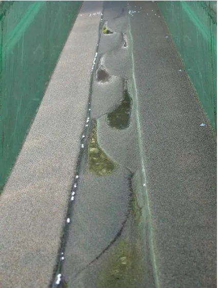
3.2 A step of the evolution of the channel: a slow meandering channel displaying

regular width variations. . . 37

(13)

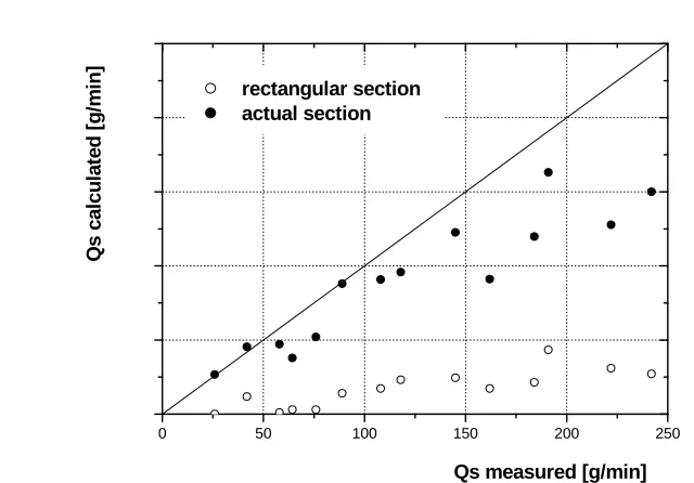
3.4 Comparison between the measured solid discharge and that calculated according

to two different estimates of the Shields stress. . . 39

3.5 Formation of alternate bars in the early stage of channel development. . . 40

3.6 Example of sorting pattern for three stages of channel development in bimodal sediment. Dark regions denote the accumulation of coarse particles. . . 41

3.7 Comparison between the measured values of bar hight and theoretical predictions of Colombini et al. (1987). . . 42

3.8 The amplitude of leading components of the Fourier spectrum of bed topography measured at three subsequent stages (t1, t2, t3) during the experimental run A1.5-10. 43 3.9 Comparison between the amplitude of alternate bars and that of transverse modes 2 + 3 in the initial stage of experimental runs. . . 44

3.10 Comparison between the amplitude of alternate bars and that of transverse modes 2 + 3 at the onset of the bifurcation. . . 44

3.11 Threshold values of the width ratio for the occurrence of different river regimes according to linear stability analysis. . . 45

3.12 Examples of the planimetric development in a slow run and in a fast run. . . 46

3.13 Comparison between the wave numbers of bars (λb) and of the bank profiles (λw). 47 3.14 The braided reach of the Sunwapta River: field campaign of Summer 2003. . . . 47

3.15 Evolution of the dimensionless amplitude of bank oscillations as a function of the width ratio. . . 48

3.16 The onset of flow bifurcation. . . 48

3.17 Peak values of the dimensionless amplitude of bank oscillations as a function of Shields stress. . . 49

3.18 The central, wedge shaped deposit of coarse particles. . . 50

3.19 Angles of bifurcations measured by the planimetric configuration (left) and angles of the central deposit (right). . . 50

3.20 Bifurcation points on the plane Shields stress - width ratio. . . 51

4.1 Bifurcation in a braided river (Sunwapta River, Canada). . . 53

4.2 Picture of theπflume. . . 55

4.3 The high precision automated carriage with the monitoring equipment. . . 56

4.4 Upstream view of the ’Y’ shaped configuration. . . 57

4.5 Run F3-21: time evolution of the discharge ratio rQ, as measured by the pressure sensor device. . . 59

(14)

4.7 Sediment discharge ratio rQs (a) and slope ratio rs (b) as functions of rQ at

equi-librium. . . 60

4.8 Sample longitudinal profiles of the downstream branches (run F3-21). . . 61

4.9 The dimensionless ’inlet step’ ∆ηas a function of Shields stress (a) and width

ratio (b). . . 61

4.10 Relationship between the discharge ratio rQ and the inlet step∆η. . . 62

4.11 Two examples of a perturbation of the equilibrium in the case of symmetrical (a)

and asymmetrical (b) configuration. . . 62

4.12 Pictures and bed topography maps of the upstream channel. Initially free migrat-ing bars (a) and steady longer bars caused by the bifurcation (b). . . 63

4.13 Two examples of runs affected by bar migration: (a) balanced run F7-24, (b)

un-balanced run F7-08. . . 64

4.14 Discharge ratio in the downstream branches rQ as a function of Shields stress. . . 65

4.15 Difference in bed elevation∆ηas a function of the aspect ratio. . . 66

4.16 Discharge ratio in the downstream branches rQ as a function of the relative dis-tance from resonant conditions. . . 67

4.17 The inlet step∆ηas a function of the relative distance from resonant conditions. . 67

5.1 A proglacial braided river, Val Martello, South Tyrol, Italy. . . 69

5.2 Study location map showing the field site on the Ridanna Creek. . . 72

5.3 The braided reach of the Ridanna Creek at Aglsboden, with the three main

mor-phological regions. (Aerial orthoimage referring to year 2000; courtesy of Bolzano local River Authority). . . 74

5.4 The conductivity meter. . . 76

5.5 Flow rating curve of the Ridanna Creek at the gauging station located at the

up-stream end of the surveyed reach. . . 76

5.6 Recorded discharges during summer 2003. . . 77

5.7 Concentration waves measured on the left and right banks. (Right downstream

channel of bifurcation 2 in the Ridanna Creek, August 16th. Q=0.22 m3/s. . . . 77 5.8 The propeller (a) and electromagnetic (b) current meters. . . 78

5.9 The ’gravelometer’. . . . 78

5.10 Images taken from the automatic digital camera. a) on August 14th at 14.00, Q=

(15)

5.12 Location of the camera station and area covered by the photogrammetric survey

(a) and control target (b). . . 81

5.13 A three-dimensional view of the DEM obtained with the digital photogrammetry. Downstream region of the Ridanna Creek, summer 2003. . . 82

5.14 Orthoimage of the central region of the study reach. . . 82

5.15 Planimetric configuration of the Ridanna Creek in July 2002, acquired with the thermograph. White dash lines represent the paleo-river beds. . . 83

5.16 Map of the study reach in which the color scale is related with the grain size. . . 84

5.17 Location of the Sunwapta field study. . . 85

5.18 View of the study reach from the cliff on the right side of the river. . . 86

5.19 Orthoimage of the study reach taken on July 26th. . . 87

5.20 The UDG station used for free surface level measurements. . . 87

5.21 Free surface level at the UDG station during the field work. . . 88

5.22 Values of discharge measured with the propellers (close symbols) compared with the UDG gauging converted into discharge (solid line). . . 89

5.23 Rating curve of the Sunwapta River at the UDG station. . . 90

6.1 Sketch and notation of a bifurcation. b is the channel width, S the longitudinal slope. 92 6.2 Location of the three monitored bifurcations on the Sunwapta River (orthorectified image taken on July, 26th, 2003). . . 93

6.3 Location of the four monitored bifurcations on the Ridanna Creek. . . 94

6.4 Picture of the four bifurcations monitored on the Ridanna Creek (images taken during summer 2003. . . 95

6.5 Measured values of the discharge ratio rQ in four bifurcations both on the Sun-wapta River (open symbols) and on the Ridanna Creek (close symbols). . . 97

6.6 Relationship between the discharge ratio rQ and the total discharge Qa as mea-sured in a laboratory test. . . 98

6.7 Transverse profiles of the velocity at bifurcation IV. . . . 99

6.8 Cross sections near bifurcation IV. a) 3 m upstream; b) at bifurcation; c) 3 m downstream. The dashed lines with close symbols correspond to bed elevation, while straight lines denote water surface level. . . 100

(16)

6.11 Orthoimage of the region interested to planimetric changes. The line indicates the

diagonal front of the alternate bar. Flow is from left to right. . . 102 6.12 Orthoimages of the study reach before (left) and after (right) the changes on

Au-gust 1st. Flow is from left to right. . . 103 6.13 Particular of the bifurcations I, II and III. Pictures taken on July 24th_{(a), August}

4th(b) and August 11th(c). Flow is from left to right. . . 103

6.14 Planimetric evolution of region A, reported on the orthoimage of September 2000. 105 6.15 Planimetric configuration of region B in 1990 (a), 1999 (b), 2000 (c) and 2003 (d).

The area where the first bifurcation occurs is pointed out. . . 106

6.16 Local free surface slope for the main channel (close symbols) and for the sec-ondary channel of region A (open symbols). . . 107

6.17 Grain size distribution along the reach. The d50(close symbols) and the d84(open

symbols) are reported. . . 108 6.18 Longitudinal variation of the braiding index of the Ridanna Creek as measured

from the aerial images taken in 1990, 1999, 2000. . . 109

6.19 Planimetric configuration of the Ridanna Creek during summer 2003: arrows in-dicate subsequent activation of the branches. . . 110

6.20 Longitudinal variation of the braiding index of the Ridanna Creek as a function of

the total discharge (m3/s). . . . 110 7.1 Observed bifurcation configurations on the width ratio / Shields stress plane. . . . 112

7.2 Comparison between experimental and computed values of the inlet step (α=3). 113

7.3 Comparison between the measured and the computed values of the inlet step of natural bifurcations. . . 113

7.4 The weakly meandering main channel of the Ridanna Creek, with a complex bar

system. (flow is toward the camera) . . . 114

(17)

List of Tables

3.1 Experimental conditions of the performed runs. . . 35

4.1 Relevant parameters for theπflume experiments. . . 58

6.1 Summary of the bifurcations data measured on the Sunwapta River. . . 96

6.2 Summary of the bifurcations data measured on the Ridanna Creek. . . 96

(18)

(19)

1 Introduction

Rivers are an important resource that can be managed at best only considering a broad range of

factors (morphological, biological, social, human, ...) in an integrated view. River training and management reflect the needs of a particular society at a certain stage of its evolution; in recent

years local conditions, which allow for cost-effective solutions and sustainable strategies have

become more and more important. Further river management activities are required to achieve traditional aims such as flood protection, maintenance of bank stability, prevention of efficiency of

water intakes. In addition, one has also to consider the restoration of all the functions of the river

system and the maintenance of instream and floodplain habitats. In this context, the concept of leaving room for the rivers is one of the key points of refurbishment projects, leading to nature and landscape restoration (de Vriend, 2002). Also the issue of vertical and lateral connectivity within

the fluvial system has gained an increasing relevance, because of its influence on groundwater resources and on pollutant dispersion and its interaction with ecological aspects and biota.

This approach can also guarantee the extra benefit of a more successful prevention system of

flood damages. In fact, the continuous rising of the main levees does not seem to be the best

solution: high magnitude flood events in the last decade (Mississippi, 1993 and Rhine, 2002) showed that an absolute safety cannot be warranted, even in very regulated rivers. On the

con-trary, confinement between embankments implies a higher unit stream power leading to disastrous

(20)

consequences when embankments fail, hence increasing flood damages (Gilvear, 1999). Novel

approaches are currently under investigation, like the enhancement of water storage in more up-stream part of the river basin, the removal of some bank protections, the re-opening or creation of

secondary channels along the main branch (Klaassen et al., 2002).

In this process, fluvial geomorphology can decisively improve river engineering techniques

in order to minimize flood damage and, at the same time, to reduce environmental degradation,

restoring ecologically valuable and aesthetically pleasing water courses (Larson, 1996). In partic-ular, a geomorphological approach can be relevant to highlight how river systems respond to water

and sediment inputs from the upstream catchment and to point out the sensitivity of geomorphic

systems to environmental disturbances and change (Gilvear, 1999).

1.1

Braiding phenomena

Braiding is one of the natural river patterns that appears over a wide range of scales, from small proglacial gravel-bed streams to large fluvial systems as the Brahmaputra River; it can be easily

described as a network of channels, splitting and rejoining around islands and bars (Figure 1.1

and 1.2). Murray & Paola (1994) defined the braided pattern as "the fundamental instability of laterally unconstrained free-surface flow over cohesionless beds". Braiding is a complex system of channels interconnected by nodes (namely, confluences and bifurcations), acting on a wide

range of spatial scales, from the single chute and lobe unit till the whole braided belt.

At present, few examples of fully braided reaches can be find in Europe, where in the past

the high land demand and the flood protection strategies led to river confinement and restricted the planimetric evolution of fluvial belts. In Italy some piedmont rivers, like the Piave River,

experienced incision and narrowing processes in the last decades (Surian & Rinaldi, 2003); in this

context the Tagliamento River, North-East Italy, is one of the latest large braided streams in Europe

(21)

Figure 1.3: The Brahmaputra-Jamuna River, Bangladesh (on the left) and the Kali Gandaki River, Nepal.

and it is considered a fluvial corridor with a great ecological and environmental relevance (Figure

1.1). Braiding is more common in regions characterised by a lower human pressure, like Canada

and New Zealand, and in the developing countries (in Figure 1.3 two examples are shown: the Brahmaputra-Jamuna River in Banghladesh, on the left, and the Kali Gandaki River in Nepal); in

this case their management is quite problematic, due to the high bank erosion rate and the highly

dynamic behaviour; hence the challenge is to develop sustainable techniques that meet local needs.

According to the new perspectives of river management presented above, braiding can be seen

as one of the target patterns of recent river engineering projects, with the aim of promoting the

restoration of the river functions. An attempt has been recently pursued with the re-opening of the secondary branches on the Rhine River. For these reasons the issue of predicting the planimetric

and altimetric evolution of a channel network has gained a greater relevance in the last decades.

Indeed, the present knowledge on river dynamics allows to predict the evolution of a single thread meandering channel, even on relatively long time scales, with sufficient accuracy and to interpret

many unit processes acting in rivers. However, understanding and predicting braiding phenomena

is still an ongoing task (Jagers, 2003).

Two different approaches have been recently pursued: the first, termed ’reductionism’

accord-ing to Paola (2001), is founded on the classical mechanical approach and comprises both numerical

(22)

on the idea of ’emergent’ phenomena: it considers that in a multi-scale system the behaviour at a

given level may be controlled by only few crucial aspects of the next level below in the hierarchy of scales; this implies that such a model may become simpler, in spite of the system complexity.

In this approach the attention is mainly focused on the general properties of the system, looking for spatial and temporal structures.

A first question to tackle when analysing a braided network is to determine how much braided it is. The most common quantification of braiding intensity, based on the number or length of the

channels within the reach, can be represented by the braiding index, given in terms of the average number of anabranches across the river (Bridge, 1993) or by the total sinuosity, defined as the

intrinsic length of channel per unit length of river. Recently, Ashmore (2001) pointed out that

the active braiding intensity can actually be very low, with only 1 or 2 channels simultaneously active. In an experimental study Stojic et al. (1998) investigated the time evolution of a braided

network through the analysis of a series of DEMs of bed topography, acquired using digital

pho-togrammetry. The authors showed that, on a short time span, deposition and erosion occur only in few channels, thus implying that the evolution of the braided pattern can be interpreted as the

his-tory of channel shifting more than the result of the interaction of simultaneously active channels.

As a result, the distinguishing features of braiding compared with single thread channels are the rapid channel shifting and the high rates and frequencies of changes in bed topography, with the

tendency of radical readjustment of the channel pattern (Ashmore, 2001).

Sediment transport reflects this highly dynamical evolution: as widely reported (Hoey &

Sutherland, 1991; Hoey, 1992), the dynamics of braided rivers is characterised by rapid spatial and temporal variations of the bed material transport rate, over a broad range of frequencies. As

an example, the sediment transport rate measured at the downstream end of a laboratory model

is reported in Figure 1.4 (Warburton & Davies, 1994). These fluctuations have been related to single dynamical processes, like the migration of bars (on the meso-scale) and to the reshaping

of the network configuration through channel migration, creation and obliteration of channels and

nodes (on the macro-scale). It has been observed (Ashmore, 1988) that a higher stream power could enhance more frequent breakdown of the morphology, thus increasing the fluctuations of

the bedload.

Paola (2001), tackling this aspect from an alternative point of view, based on the results of the

cellular model of Murray & Paola (1994), highlighted how the non linear response of sediment transport to variation in water flux is essential in developing a braided pattern. More specifically,

the ’over-response’ of sediment flux to acceleration in the confluences and deceleration in the

diffluence areas promote continuous bed scouring and deposition of bars, so that ’bed and flow chase one another forever around the braid plain’.

(23)

Figure 1.4: Bedload transport rate fluctuations in a braided laboratory model. Plot reported in Warburton & Davies (1994).

of Howard et al. (1970). A research line on braiding deals with the investigation of internal

ge-ometric similarity: it has been found that braided rivers show scale invariance, i.e. they display

similar statistical properties independently of the spatial scale, if they are not subject to external controls. More precisely, Sapozhnikov & Foufoula-Georgiou (1996) demonstrated that braiding

can be considered a self-affine object, since it has a preferential direction (that of the mean

down-stream flow). This maight imply that the underlying mechanisms responsible for the formation of braiding are the same at all scales.

Indeed, the characteristic scales of braided rivers and their relationship with morphological parameters as water discharge, mean valley slope and grain size are still not completely

under-stood. Braided channel width can be considered as the sum of the width of the single anabranches

or represented by the width of the braid belt. The width of a single gravel bed channel can be evaluated following rational regime theories (Parker, 1978), but the present state of knowledge

does not allow to determine the functional controls on braided width (Warburton, 1996). Field and

laboratory data show that total width can also be a function of the braiding intensity. Ashmore (2001) recently pointed out the existence of a characteristic length scale of braiding related to the

total discharge of the river. Similarly to the relations for meander wavelength, the mean braid

(24)

1.2

Prediction of braided rivers evolution

At present, the prediction of braided rivers planform evolution is possible with enough accuracy only on a short time scale. Braiding is a deterministic system characterised by a somehow chaotic

behaviour, as it apparently shows unpredictable features (Paola & Foufoula-Georgiou, 2001).

Time evolution of the channel network is affected by rapid changes, due to the rearrangement of the branches and nodes and, in particular, caused by the modification of the flow and sediment

distribution at the bifurcations. The standard approach that solves the governing equations for

the fluid and solid phases (Enggrob & Tjerry, 1999; McArdell & Faeh, 2001) encounters various difficulties arising from the complexity of the system. Such a model has to deal with a

continu-ously changing domain and requires the full coupling between bed and bank evolution. Moreover,

secondary flows, sorting effects and local turbulence disequilibrium have to be accounted for. Fur-thermore, braided rivers are characterised by several complicating features that must be taken into

account by theoretical modelling. Principally:

• Strong non-linearities: the planimetric and altimetric evolution of the branches is affected by the interaction between the free bed-response of the system and the forced bed-response

due to planform non-uniformities.

• Unsteadiness: flow field and sediment transport rate are typically unsteady and the system never reaches a steady equilibrium configuration.

• Finite length and amplitude effects: the relatively short length of single anabranches implies that the condition of infinite longitudinal domain, which is often introduced in theoretical models, can be hardly met in nature; as a consequence, upstream and downstream

mor-phodynamic influence may crucially affect the evolution of single branches. Moreover, bar

structures generally undergo a finite amplitude development, thus limiting the applicability of linear theories.

• Partially transporting cross sections and gravitational effects: braided rivers are generally characterised by low sediment mobility, near the threshold value for particle motion, which implies that sediment transport may occur only on a limited part of the cross section.

More-over, gravitationally effects on sediment transport are likely to be relevant due to the fairly

large bed gradients associated with local depositions and scours.

To overcome the above complications other alternative models for braiding have been recently

developed. Murray & Paola (1994) have shown that a simple cellular model, which includes only

(25)

Figure 1.5: Cellular routing scheme of the Murray & Paola (1994) model.

the cellular routing scheme is reported). Though the above model was not designed to predict

the actual planform changes, it is able to recognise some fundamental aspects of braided systems. Following a similar approach, Thomas & Nicholas (2002) have recently proposed an improved

version of the cellular routing scheme, which has been tested with field data and compared with a

more detailed 2D hydraulic model.

Jagers (2003) has tackled the problem of modelling planform changes in braided rivers. He has implemented two different models, a neural network and a branches model, testing their accuracy

with observed data from the Brahmaputra-Jamuna River (Figure 1.6).

The branches model is based on a schematisation of the braided river as a network of channels,

joining at the nodes (confluences and bifurcations). Each individual ’object’ evolves according to

four processes, namely width variation, mid-channel bar formation (and therefore creation of a new channel), lateral migration or channel abandonment. The spatial distribution of erosion and

deposition probabilities is then computed from the results of a Monte Carlo simulation. Such a

model seems to be very promising in predicting medium and long term evolution of a braided system. The main limitation is due to the difficulty in setting the correct values of parameters

underlying the single evolution processes. For example, the creation of new channels is only

accounted for through the mid-bar formation mechanism, provided a threshold value of the width to depth ratio of the channel is exceeded.

According to Paola (2001) a mixed model that combines both the reductionist and the syntesist

point of view could be envisaged; such a model, essentially a ’two layers’ model, could include

(26)

Figure 1.6: Comparison between the predictions obtained through the branches model, the neural network and the observed erosion sites on the Jamuna River. (From Jagers, 2001).

1.3

The unit process of bifurcation

Braiding is generated and maintained through the mechanism of flow bifurcation (see Figure 1.7 and the cover picture, taken from the Tagliamento River, Italy). Bifurcation is the process that

determines the distribution of flow and sediments along the downstream branches and adds

com-plexity to the system, thus reducing its predictability. Modelling a bifurcation is still a challenge for existing mathematical models, even in a simple configuration (Klaassen et al., 2002): hence,

understanding river bifurcation is one of the open issues of fluvial research.

In order to model channel adjustment and to locate the preferential bank erosion areas and the

probability of scour or deposition, the preliminary understanding of the mechanisms underlying the onset of the flow diffluence is required. Furthermore, the knowledge of the morphology and

hydraulic conditions typical of a bifurcation allows one to know the water end sediment partition within the network. The availability of quantitative detailed description of the bifurcation process

could ensure a decisive improvement in the ability of theoretical models to predict the planimetric

and altimetric evolution of a braided river; moreover, such knowledge could be significant also in the context of other morphological pattern, as anastomosing and pseudo-meandering rivers.

A quantitative description of river bifurcation process is still lacking in the literature. The

process has been firstly identified by Leopold & Wolman (1957) as the generating process of

(27)

Figure 1.7: A bifurcation on the Sunwapta River, Canada. Flow is toward the camera.

• Central bar mechanism and dissection of transverse unit bar. This mechanism (also docu-mented by Leopold & Wolman, 1957) imply the development of a central bar, displaying an

avalanche faced downstream margin marked by the accumulation of the coarsest fractions.

The bar forces the flow to diverge and is eventually exposed. A similar mechanism, with the dissection of a transverse unit bar may occur, when the channel is characterised by a higher

sediment mobility.

• Chute cutoff mechanism. It is the most common bifurcation mechanism observed in the experiments; it is characterised by the modification of a an alternate bar structures in

low-sinuosity channels. The bar is progressively transformed into a more complex bed form by lateral accretion, which determine more flow to be directed over the point bar. The steeper

gradient near the head of the slough channel captures progressively larger volumes of water,

leading to the bifurcation of the flow.

• Multiple bars mechanism. This mechanism applies only to channel with very high values of the width/depth ratio; it has been documented by Fujita & Muramoto (1988) and can be roughly explained in terms of the results of the linear stability analysis (Fredsøe, 1978). The

multiple rows bars, which characterise the initial bed configuration, are gradually converted

into fewer larger bars which concentrate the flow and lead to braiding.

The bifurcation process has been recently investigated also by Federici & Paola (2003) through experiments performed in divergent channels. They have found that stream lines diffluence

invari-ably promotes the formation of a central deposition area, leading to the bifurcation of the current.

(28)

Figure 1.8: Alternating point bar chute cutoff mechanism, as reported by Ashmore (1982).

the bifurcation is stable, with both branches active; on the contrary, low sediment mobility leads

to the closure of one of the branches. The authors notice that this ’switch’ configuration is also triggered by the non uniformity of initial and boundary conditions: in fact, a flow perturbation can

influence the stability of the bifurcation.

A predictive model for the equilibrium configuration of a simple ’Y-shaped’ configuration in

which an upstream channel divides into two branches has been proposed by Wang et al. (1995). The problem has been recently revisited by Bolla Pittaluga et al. (2003) through the introduction

of a quasi-2D nodal condition that allows for transverse exchanges of water and sediment within

the final reach of the upstream channel that feeds the bifurcation. The results of the model suggest the possibility of unbalanced equilibrium configurations, even in the case of perfectly

symmet-ric geometry. The unbalanced solutions appear for low values of the sediment mobility and high

values of the width to depth ratio; they are characterised by an unbalanced discharge ratio in the downstream branches and by a difference of bed elevation at the inlet of downstream branches.

In spite of the simplified one-dimensional schematisation adopted by Bolla Pittaluga et al. (2003),

(29)

Finally, it is worth noticing that understanding complex system like a braided network needs

an integrated analysis, which allows one to deal with different spatial and temporal scales. Hence, it is highly recommended to join the information obtained through by theoretical analysis with

data from laboratory and field investigations.

1.4

Outline of the thesis

In the present work the attention has been focused on the bifurcation process with the aim of describing quantitatively the flow conditions that lead to flow bifurcation and then determining its

equilibrium configurations. The analysis is mainly based on experimentally and field observations:

two different experimental works in the Hydraulic Laboratory of the University of Trento have been performed; further, two braided reach have been intensively monitored, paying particular

attention to the analysis of bifurcations. Measured data have been integrated and interpreted with

reference to theoretical results.

In summary, through the present work we have tried to address to the following questions:

• Which are the flow conditions that lead a laterally unconstrained channel to bifurcate?

• How can the chute cutoff mechanism be interpreted in the viewpoint of interaction and modification of bar structures?

• Is it possible to define a characteristic length scale of braiding based on bar analysis?

• Which are the main features characterising the equilibrium configuration of a bifurcation?

• Up to what extent such equilibrium configuration is affected by bar migration and/or up-stream and downup-stream morphodynamic influence?

• What is the role played by bifurcations in controlling the planimetric evolution of a braided network?

(30)

The thesis is organised as follows.

In Chapter 2 a brief review of the theoretical framework is reported, focusing the attention on single unit processes as bar formation and on the response of bed topography to planform non

uniformities; a predictive model for channel bifurcation is also presented in Section 2.4. Chapter 3 is devoted to the experimental analysis of the bed and bank evolution of a single channel, until the

onset of the bifurcation. Altimetric and planimetric configuration is analysed in detail to describe

flow conditions at the moment of incipient bifurcation. In Chapter 4 the experimental investigation of a ’Y-shaped’ configuration is reported; the results of two sets of runs allow to characterise the

equilibrium configuration of a bifurcation and to highlight the role of the width to depth ratio on

the degree of asymmetry of the discharge distribution. The field campaigns on the Ridanna Creek and on the Sunwapta River, the measurement techniques and the obtained data on bifurcations

and planimetric evolution are described in Chapters 5 and 6. Finally, Chapter 7 is devoted to the

(31)

2 Theoretical framework

2.1

General formulation

Bed deformation in single thread channels may be due to spontaneously developing bedforms or to

the forced pattern induced by planform non-uniformities. The subject has been widely investigated in the last decades (state of the art reviews can be found in Seminara, 1995; Tubino et al., 1999;

Bolla Pittaluga et al., 2001). In particular, the ’mechanical’ approach has been quite suitable

for the understanding of the basic mechanisms characterising river morphodynamics, namely the formation of bars in straight channels, the bed deformation in meandering channels or in channels

with variable width.

A suitable form of the governing equations for the liquid and solid phases can be obtained, introducing reasonable simplifying hypotheses which can be set once the relevant temporal and

spatial scales have been identified. In the present work we focus our attention on processes scaling

on the channel width (macro-scale bed forms); this enables us to use a two-dimensional form of the shallow water equations (the channel is generally assumed to be wide enough to neglect side

boundary effects.)

Moreover, we assume that the temporal scale of bed evolution is much greater than the time scale of the flow; hence we ignore the time-derivatives in the momentum equation. A further

quite restrictive hypothesis allows us to decouple the planimetric development and the altimetric evolution, provided the latter occurs on a much faster time scale. This approximation can be

reasonable in the context of single thread meandering channels with cohesive banks, while it is

not always justified in gravel bed rivers, where bed and banks may evolve at nearly the same time scale, particularly when a braided pattern establishes.

In a standard depth-averaged model the effect of secondary flows is neglected, because of the

vanishing of the net contribution when averaged over the depth. Indeed, secondary flows are quite relevant to determine many of the features displayed by bed configurations. The decomposition

originally proposed by Kalkwijk & De Vriend (1980) can be introduced to account for their effect

(32)

v=νovo(ζ,n,s) +V(n,s)

F

o(ζ), (2.1)

u=

F

o(ζ)U(n,s), (2.2)

where s is the longitudinal coordinate, defined along the channel axis, n is the transverse

coordinate, νo=b/Ro is the curvature ratio, and reference is made to a channel whose width b

remains nearly constant, while the curvature of channel axis may change arbitrarily, Ro denoting

a typical (average or maximum) value of the radius of curvature.

Furthermore,ζis a boundary fitted vertical coordinate

ζ=z−η(s,n)

D(n,s) , (2.3)

whereηand D denote the local values of bed elevation and flow depth, respectively, and U and V are the depth-averaged components of velocity in longitudinal and transverse direction,

respectively.

The decomposition 2.1 and 2.2 essentially implies that the effect of centrifugally induced

secondary flow vo, whose depth average vanishes, can be locally added to the depth averaged

component, whose vertical structure

F

o(ζ)is assumed to coincide with the standard distribution

of uniform flow evaluated in terms of the local flow characteristics.

Notice that a broader formulation which also accounts for the effect of the variable width has

been recently proposed by Andreatta et al. (2004).

A suitable scaling can be introduced in the analysis, using the half channel width for the

longitudinal and transverse coordinate and introducing reference values of velocity Uo and depth

Do as the values corresponding to a uniform flow, for given values of flow discharge, channel

width, average bed slope and sediment size.

Once the above scaling is adopted, the following relevant dimensionless parameters arise:

• the width to depth ratio (or aspect ratio) of the channel

β= b

2Do

; (2.4)

• the Shields stress

ϑ= τo

[(ρs−ρ)gDs]

(33)

whereτo is the average bottom shear stress, ρs andρare sediment and water density,

re-spectively, g is gravity and Dsis a typical grain size;

• the relative roughness

ds=

Ds

D . (2.6)

Referring to an orthogonal reference system (s,n,z)with s longitudinal coordinate, n trans-verse coordinate defined along a horizontal axis orthogonal to s and z coordinate of the axis

or-thogonal to s and n and pointing upwards, the governing equations of the two-dimensional model assume the following form:

UU,s+VU,n+H,s+β τs

D = νof11+O(ν

2

o), (2.7)

UV,s+VV,n+H,n+β τn

D = νog11+O(ν

2

o), (2.8)

(DU),s+(DV),n = νom11, (2.9)

(F_o2H−D),t+Qo[qs,s+qn,n] = νon11, (2.10)

where H is free surface elevation, Qois a dimensionless parameter defined as:

Qo=

p

(s−1)gD3

s

(1−p)UoDo

, (2.11)

where s is the relative density and p sediment porosity and Fois the Froude number. Moreover τsandτnare the longitudinal and transverse components of the bottom stress vector, while qsand

qnare the longitudinal and transverse components of the bedload transport; in the case of a slowly

varying bed topography they can be evaluated through the semi empirical relationship (Shimizu et

al., 1992):

q= qo(ϑ)

τ {τs[cos(α),sin(α)] +τn[−sin(α),cos(α)]}, (2.12)

tan(α) =− r

β√ϑ

∂η

∂y , (2.13)

where the angleαdescribes how gravity, acting on particles moving on a sloping surface, affects the direction and intensity of bedload motion, driving some deviation of the average particle

trajec-tory from the direction of mean bottom stress. Furthermore, y is orthogonal to the local direction

of bed stress and r is an empirical constant ranging between 0.3 and 0.6 (e.g. Talmon et al., 1995).

(34)

(2.7-2.10) account for the effect of centrifugally induced secondary flow and of dispersive terms

related to its interaction with the topographically induced variations of the depth averaged flow.

2.2

Alternate bar formation

River bars are fundamental features which control the evolution of alluvial channels (Figure 2.1).

Their formation has been conclusively explained in terms of an inherent instability of an erodible

bed. The solution of system (2.7-2.10) in the case of a straight channel (νo =0) allows one

to determine the occurrence conditions and the equilibrium configuration of migrating alternate

bars. The problem has been tackled through linear and weakly non linear analytical approaches

(Colombini et al., 1987; Tubino et al., 1999), fully non linear models (Colombini & Tubino, 1991; Schielen et al., 1993) and various experimental analyses (Jaeggi, 1984; Fujita & Muramoto, 1985;

Garcia & Niño, 1993; Lanzoni & Tubino, 2000).

The results of the above investigations are presented and briefly summarized in the following. The theoretical plots presented herein are obtained using the Parker (1990) formula to compute

the bed load function qo appearing in 2.12, which allows one to obtain more accurate predictions

at low values of Shields stress, typical of braided networks.

Field and experimental observations suggest that the longitudinal wave length of alternate bars fall in the range of 5-12 channel widths (Figure 2.2a). Furthermore, their equilibrium height,

which is defined as the difference between the maximum and minimum bed elevation within a bar

unit, increases as the width ratio of the channel increase, as shown in Figure 2.2b.

(35)

0 5 10 15 20 25 30

0 5 10 15 20 25 30 35

width ratio w a v e l e n g th / c h a n n e l w id th 0 1 2 3 4 5 6

0 5 10 15 20 25 30 35 40 45

width ratio b a r a m p li tu d e

Figure 2.2: Observed values of the bar wave length (on the left) and of the bar height (on the right) as a function of the width ratio.

0.1 0.2 0.3 0.4 0.5

5 10 15

β_c _0.001

0.05 0.03 0.02 0.005 0.1 d_s

Figure 2.3: The critical value of width ratioβc predicted by the linear model of Colombini et al. (1987) as a function of the Shields stressϑand the relative roughness ds.

Indeed, linear studies suggest that the bifurcation parameter for bar instability is the width

ratio: in Figure 2.3 the threshold value of the width ratio above which the occurrence of alternate

bars is reported, as predicted by the linear model of Colombini et al. (1987).

Linear theories also show that the instability process is not strongly size-selective: the shape

of marginal stability curves (Figure 2.4) suggests that different waves within the unstable range

modes are characterised by almost similar growth rate.

On the contrary, the transverse mode selected by the instability process depends strongly on β; as a consequence, free bar instability generally displays an alternate pattern (mode 1), while central bars (mode 2) or multiple row bars (mode 3, 4, ...) can only form when the channel is

fairly wide. As firstly pointed out by Fredsøe (1978), the critical condition for a given transverse

mode m is given by mβc,βc being the threshold value for alternate bars (Figure 2.5).

(36)

5 6 7 8 9 10 11 12 13 14 15

0 0.2 0.4 0.6 0.8 1 1.2 1.4 1.6 1.8 2

wave number w id th r a ti o ββββc Ω Ω Ω

Ω = 0

FREE ALTERNATE BARS

PLANE BED

Figure 2.4: Marginal stability curve predicted by the linear theory (Shields stress = 0.07, relative roughness = 0.01).

0 0.2 0.4 0.6 0.8 1 1.2 1.4 1.6 1.8

0 10 20 30 40 50 60

width ratio Ω / Ω Ω / Ω Ω / Ω Ω / Ωm a x 1 MODE 3 MODE 2 MODE 1

βc βc2 βc3

Figure 2.5: The growth rateΩmax is plotted versus the width ratio for different transverse modes. (Shields stress = 0.07, relative roughness = 0.05).

channel falls in a neighborhood ofβc, the weakly non linear theory of Colombini et al. (1987)

suggests that nonlinear interactions lead to periodic bar patterns migrating downstream, whose

amplitude may asymptotically reach an equilibrium value. It is found that the equilibrium bar

amplitude (HBM), scaled by the average flow depth, is proportional to the square root of the excess

of the width ratio relative to the threshold valueβc and can be expressed in the form:

HBM =b1ε 1

2+_b

2ε, ε=

β−βc

βc

, (2.14)

where b1 and b2 are functions of the Shields stress ϑ and the relative roughness ds and are

(37)

0.1 0.2 0.3 0.4 0.5 0.8 0.9 1.0 1.1 b 1 d_s 0.03 0.05 0.02 0.01 0.005 0.001

0.00 0.01 0.02 0.03 0.04 0.05 0.6 0.7 0.8 0.9 b₂ d_s 0.5 0.4 0.3 0.2 0.1 0.07

Figure 2.6: The functions b1and b2are plotted in terms ofϑand ds.

0 1 2 3 4 5 6 7

experimental amplitude of bars

th e o re ti c a l a m p li tu d e o f b a rs

Figure 2.7: The maximum height of alternate bars as predicted by the weakly non linear theory of Colombini et al. (1987) is compared with experimental data of various authors.

Comparison of predicted bar height with flume data seems quite satisfactory, as reported in

(38)

2.3

Planimetric forcing

As pointed out in Section 2.1 the bed response of a natural channel is also determined by

forc-ing effects induced by planform non uniformities, like the curvature of channel axis and width variations. The structure of the resulting bed pattern closely reflects that of the forcing effect. In

particular bed topography displays a typical alternate pattern when the forcing is anti symmetrical,

like in the case of periodic variation of channel curvature in meandering channels (Figure 2.8).

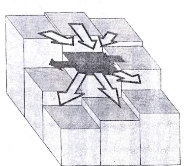
On the contrary, a ’symmetrical’ forcing like that produced by a periodically varying width is

likely to induce a sequence of central deposits whose longitudinal and transverse structure resem-ble that of central bars.

The forced bed pattern can in turn affects the process of bank erosion, thus enhancing the

further development of channel non uniformities. Both the effects of variable curvature and of symmetrical width variations have been investigated in the last decades through experimental

ob-servations and theoretical models.

Kinoshita & Miwa (1974) and Tubino & Seminara (1990) investigated the interaction between

free migrating bars and steady point bars induced by the variable curvature of channel axis,

show-ing that a threshold value for channel curvature exists, above which free bars cease their migration and bed topography is characterised by steady patterns (see Figure 2.9).

Repetto & Tubino (1999) and Repetto et al. (2002) analysed both experimentally and theoret-ically the forcing effect of symmetrical, periodic width variations. Also in this case a threshold

value of the amplitude of bank oscillation can be defined, above which alternate migrating bars

are suppressed and the bed topography displays a steady central bar pattern. In Figure 2.10 the amplitude of width variations is expressed in a dimensionless form, whereδis the amplitude of

(39)

Figure 2.9: The critical values of the channel curvature, as determined by Tubino & Seminara (1990) compared with the experimental data of Kinoshita & Miwa (1974) (open sym-bols represent migrating bars, close symsym-bols non-migrating bars).

Figure 2.10: The critical values of the amplitude of width variations as a function of the width ratio and the Shields parameter (from Repetto & Tubino, 1999).

the bank oscillations divided by the mean channel width.

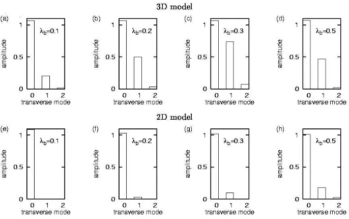
Repetto et al. (2002) also investigated the steady forced response of the system driven by

periodic width variations. In this case, the bed topography is characterised by two leading compo-nents: the former (transverse mode 0) is a purely longitudinal bed deformation, with an associated

deposition in the wide sections and scour in narrow sections, the latter (transverse mode 1) implies

(40)

Figure 2.11: Equilibrium bed configuration of a channel with variable width. (from Repetto et al., 2002).

Figure 2.12: Amplitude of the leading transverse modes of the bed topography obtained with the three-dimensional model (a-d) and the two-dimensional model (e-h). (from Repetto & Tubino, 1999).

lines curvature are fundamental to determine the occurrence of the above central bar pattern.

(41)

a two-dimensional model, which is unable to account for secondary flows, can not reproduce a

transverse bed deformation.

Furthermore, the formation of the central deposits is found to enhance the amplitude of the

width variations, in particular for low values of the bottom shear stress and for high values of the

width to depth ratio. As a result the planimetric configuration may be unstable and can lead to channel bifurcation.

2.4

Meander resonance and morphodynamic influence

In order to investigate the morphodynamics of a meandering channel the two-dimensional model

presented above (Equations 2.7-2.10) can be solved through a linear approach, taking advantage

of the fact that the curvature ratioνois typically a small parameter; hence we can set:

(U,V,D,H) = (Uo,0,Do,Ho) +νo(u,v,d,h) +O(ν2o). (2.15)

The above procedure has been widely used since the original work of Ikeda et al. (1981) (see also Blondeaux & Seminara, 1985; Johannesson & Parker, 1989; Seminara & Tubino, 1989;

Seminara & Tubino, 1992).

The linearization of the mathematical problem allows one to obtain an analytical solution: it

is worth noticing that the above solution exhibits resonant behaviour when the values of the width

ratio β and meander wave numberλ fall within a convenient neighborhood the resonant value βrandλR. The above behaviour, which has been originally detected by Blondeaux & Seminara

(1985), is displayed when the periodic variation of the curvature of the channel axis forces a non

amplifying and non migrating free response of the bed configuration (Figure 2.13).

The linear system can be reworked to obtain a non-homogeneous ordinary differential

equa-tion with constant coefficients. The characteristic exponentsλj for the first transverse mode are

reported in Figure 2.14. One of the exponents is always real and positive, one real and negative, the other two are complex conjugate. The real part of the latter is negative, provided the width

ratio is smaller than a threshold value, which, for the first mode, coincides with the resonant value βR.

The main result of the analysis is that a two-dimensional perturbation of the bed topography

is mainly felt upstream in super-resonant conditions (β>βR) while it may dominantly influence

the downstream bottom configuration in sub-resonant conditions (β<βR) (Zolezzi & Seminara,

2001).

These theoretical findings may provide an explanation of the overdeepening phenomenon

(42)

0 10 20 30 40 50 60

0 0.2 0.4 0.6 0.8 1 1.2 1.4 1.6 1.8 2

β

λ β = β_R

I

II III

III

IV

Ω = 0

ω = 0

Ω(λ)

Figure 2.13: Neutral curves for two-dimensional free bars instability (Ω =0) and migration (ω= 0). (from Zolezzi & Seminara, 2001)

0 10 20 30 40

-1.2 -0.8 -0.4 0 0.4 0.8 1.2

β λ_1j dominant UPSTREAM INFLUENCE dominant DOWNSTREAM INFLUENCE

β = β_R

λ₁ λ₂ λi 4 λ i 3 λr

3 = λr4

Figure 2.14: The four characteristic exponentsλjas a function of the width/depth ratio. Solid lines

denote the real parts of the exponents while dotted lines denote their imaginary parts. (from Zolezzi & Seminara, 2001)

sharp change in channel curvature (Figure 2.15) leads to the formation of a steady pattern of

alter-nate bars in the upstream reach or in the downstream reach provided the flow is in super-resonant

or sub-resonant condition, respectively. Experimental observations on a U-shaped channel by

Zolezzi et al. (2004) confirm the above behaviour. A similar effect is determined by an

(43)

Figure 2.15: Overdeepening: sketch of the channel. (from Zolezzi & Seminara, 2001)

-80 -40 0 40 80

-80 -40 0 40 80 120 160 200 240

y/B

x/B 1

2

3

-80 -40 0 40 80

-120 -80 -40 0 40 80 120 160 200

y/B

x/B 1

2 3

Figure 2.16: Sub-resonant (left) and super-resonant (right) evolution of periodic meanders. (from Seminara et al., 2001)

According to Seminara et al. (2001) sub-resonant and super-resonant conditions also affect the planimetric evolution of a meandering channel, as shown in Figure 2.16. In particular, the

maximum erosion rate shifts from downstream to upstream of the bend apex, when crossing the

(44)

2.5

A predictive model for channel bifurcation

The analysis of the equilibrium configuration and stability of a single bifurcation has been

re-cently tackled by Wang et al. (1995) and Bolla Pittaluga et al. (2003) within the context of a

one-dimensional model. They considered a simple geometry (see Figure 2.17) with one channel (labelled a) that bifurcates into two symmetrical branches (labelled b and c). All branches have

constant width and slope and are in equilibrium with some given water discharge Q and sediment

discharge Qs.

Within the framework of a one-dimensional model with mobile bed, five nodal conditions are

needed at the bifurcating point; in particular unlike in the case of confluences, a relationship is required, which governs water and sediment distribution in the downstream branches. Wang et al.

(1995) introduced an empirical nodal points condition.

bbqs,b

bcqs,c

= µ

Qb

Qc

¶_kµ bb

bc

¶₍₁₋_k₎

, (2.16)

with qs sediment transport rate, b channel width and Q water discharge in the downstream

branches b and c.

The authors found two possible equilibrium configurations: in the first one both branches are

open, in the second one of the downstream channels is closed. The stability of the two solution was

found to be strongly affected by the empirical parameter k, whose determination is quite difficult, because it is neither related to the hydraulic conditions nor to the bifurcation geometry.

To overcome the above difficulties Bolla Pittaluga et al. (2003) proposed an alternative nodal point condition, based on a quasi two-dimensional approach. The authors divide the last reach of

the upstream channel (for a length equal toαba, where b is the channel width) in two cells

(Fig-ure 2.18). The water and sediment discharges are considered uniformly distributed in the cross section; hence, the discharges into the two ending cells are proportional to their width. Lateral

exchanges of both water and sediments are also possible. In particular, based on a generalised

(45)

version of Equation 2.12, the transverse sediment discharge is evaluated as the sum of two

con-tributions: the first is due to the fact that a transverse component of flow velocity may establish at the bifurcation due to bed deformation, which also implies a transverse exchange of sediments;

the second contribution depends on the transverse bed slope; hence, the transverse exchange of sediment can be given in the following form:

qy=qa

· QyDa

QaαDabc

−√r ϑ

∂η ∂y ¸

, (2.17)

where

Qy=

1 2

µ

Qb−Qc−Qa

bb−bc

bb+bc

¶

, (2.18)

Dabc=

1 2

µ

Db+Dc

2 +Da

¶

, (2.19)

and q is the sediment discharge per unit width, D is flow depth,ϑthe Shields parameter,ηthe bed elevation and the subscripts a,b,c identify the channels. The lengthαbaprovides a measure

of the upstream reach within which the effect of the bifurcation is felt; experimental findings by

Bolla Pittaluga et al. (2003) suggest thatαis an order-one parameter.

With such a nodal condition Bolla Pittaluga et al. (2003) investigated the possible equilibrium configurations of the bifurcation. The main results are reported in Figure 2.19. Here the

equi-librium discharge ratio of the downstream branches is shown, as a function of the width to depth

ratio of the upstream channel a for different values of the Shields parameter. A symmetrical so-lution invariably exists, whereby the same discharge flows within the downstream channels. For

(46)

Figure 2.19: Equilibrium configurations of the bifurcation as determined by the model of Bolla Pittaluga et al. (2003). (a) Discharge ratio in the downstream branches as a function of the width to depth ratio of the upstream channel. (b) Separation lines between the region with one possible solution and three equilibrium configurations.

relatively high values of the width/depth ratio two further configurations occur, characterised by a strongly unbalanced water distribution. When a multiple solution exists, the symmetrical state

is invariably unstable. Figure 2.19b shows that a unique balanced configuration can be obtained

when the sediment mobility is high or when the width to depth ratio is quite small. The unbalanced configuration is also characterised by different bed elevations at the inlet of the downstream

chan-nels, the channel that carries more water showing a lower bed elevation. These results are in fairly

good agreement with the results of the experimental investigation of Federici & Paola (2003), who found stable bifurcation in a divergent channel only when the Shields parameter attains relatively

high values.

We may notice that field observations suggest that natural bifurcations generally exhibit an

unbalanced configuration and, at the same time, different widths of the downstream branches

(see Chapter 6). Hence, the theory should be extended in order to the case of self-formed channel, whose geometry may adjust to hydraulic conditions. An attempt in this direction has been recently

pursued by Miori et al. (2004). Such analysis preliminarily requires the introduction of suitable

’regime’ equations able to define an equilibrium channel width in terms of flow and sediment characteristics. Several empirical relationships of this kind have been proposed in the literature.

Here the rational formula obtained by Griffiths (1981):

b=5.28QS1.26D−_s1.5, (2.20)

(47)

Figure 2.20: Relationship between the Shields stress and width/depth ratio as determined by the equation of Ashmore (2001) (a) and Griffiths (1981) (b) (Ds=0.05 m).

b=0.087Ω0.559D−_s0.445, (2.21)

where Q is the water discharge, Dsthe mean grain size, S the average bed slope andΩis the

stream power.

The introduction of a ’regime’ relationship in the model of Bolla Pittaluga et al. (2003) implies

that the upstream values of Shield stress and width ratio are no longer independent and follow the regime relationships reported in Figure 2.20.

We notice that the proposed ’regime’ relationships provide values of the Shields stress falling

within a neighbor the threshold of the value for the incipient motion; as a consequence, bifurca-tions in self-formed channels are more likely to display an unbalanced configuration, falling in the

region where the system admits of three solutions. The model results are reported in Figure 2.21,

where the ’regime’ equation proposed by Ashmore (2001) has been used.

The equilibrium configurations are similar to that obtained with fixed channel widths; for

values of the width to depth ratio typical of gravel b