Implementation of an immersed boundary method in the Meso-NH v5.2 model: applications to an idealized urban environment

CECI-CNRS, Toulouse, France

2_{Computational Science Division and Leadership Computing Facility, Argonne National Laboratory, Lemont, IL, USA} 3_{Department of Mechanical and Industrial Engineering, University of Illinois at Chicago, Chicago, IL, USA}

4_{Centre National de Recherches Météorologiques (CNRM), Météo-France-CNRS, Toulouse, France} Correspondence:Franck Auguste ([email protected])

Received: 12 January 2018 – Discussion started: 12 March 2018

Revised: 13 May 2019 – Accepted: 3 June 2019 – Published: 1 July 2019

Abstract. This study describes the numerical implementa-tion, verification and validation of an immersed boundary method (IBM) in the atmospheric solver Meso-NH for ap-plications to urban flow modeling. The IBM represents the fluid–solid interface by means of a level-set function and models the obstacles as part of the resolved scales.

The IBM is implemented by means of a three-step proce-dure: first, an explicit-in-time forcing is developed based on a novel ghost-cell technique that uses multiple image points instead of the classical single mirror point. The second step consists of an implicit step projection whereby the right-hand side of the Poisson equation is modified by means of a cut-cell technique to satisfy the incompressibility constraint. The condition of non-permeability is achieved at the embedded fluid–solid interface by an iterative procedure applied on the modified Poisson equation. In the final step, the turbulent fluxes and the wall model used for large-eddy simulations (LESs) are corrected, and a wall model is proposed to ensure consistency of the subgrid scales with the IBM treatment.

In the second of part of the paper, the IBM is verified and validated for several analytical and benchmark test cases of flows around single bluff bodies with an increasing level of complexity. The analysis showed that the Meso-NH model (MNH) with IBM reproduces the expected physical features of the flow, which are also found in the atmosphere at much larger scales. Finally, the IBM is validated in the LES mode against the Mock Urban Setting Test (MUST) field exper-iment, which is characterized by strong roughness caused by the presence of a set of obstacles placed in the

atmo-spheric boundary layer in nearly neutral stability conditions. The Meso-NH IBM–LES reproduces with reasonable accu-racy both the mean flow and turbulent fluctuations observed in this idealized urban environment.

1 Introduction

Urbanization impacts the physical and dynamical structure of the atmospheric boundary layer, influencing both the lo-cal weather and the concentration and residence time of pol-lutants in the atmosphere, which in turn impact air quality. While the physical mechanisms driving these interactions and their connections to climate change are well understood (the urban heat island effect, anthropological effects), their precise quantification remains a major modeling challenge. Accurate predictions of these interactions require modeling and simulating the underlying fluid mechanics processes to resolve the complex terrain featured in large urban areas, in-cluding buildings of different sizes, street canyons and parks. For example, it is well known that pollution originates from traffic and industry in and around cities, but the actual dis-persion mechanisms are driven by the local weather. Further-more, fine-scale flow fluctuations influence nonlinear physic-ochemical processes. The present study addresses these is-sues by focusing on the numerical aspects of the problem.

experi-ment (JU2003), scalar dispersion was measured experimen-tally over the streets of Oklahoma City (Clawson et al., 2005; Liu et al., 2006). Similarly, the CAPITOUL experiment (2004–2005), conducted in Toulouse, analyzed the turbu-lent boundary layer developed over the urban topography and evaluated the energy exchanges between the surface and atmosphere (Masson et al., 2008; Hidalgo et al., 2008). More recently, the multiscale field study by Allwine et al. (2012) provided meteorological observations and tracer con-centration data in Salt Lake City. Other studies analyzed reduced-scale and/or idealized models to understand urban climate features as in the COSMO (Comprehensive Outdoor Scale Model Experiment for Urban Climate) and Kugahara projects (Moriwaki and Kanda, 2004). For example, Kanda et al. (2007) and Wang et al. (2015) respectively used an ar-ray of cubic bodies and stone fields as small-scale models.

In order to use these experimental data in the future for model validation, the numerical models need to first be ver-ified for academic test cases and simplver-ified scenarios repre-sentative of atmospheric turbulent boundary layer flows. In particular, flow interaction with buildings or any generic ob-stacles plays a crucial role in urban flow modeling. The range of scales of objects acting as obstacles is huge in an urban setting, encompassing large buildings and small vegetation scales, and so is the range of the corresponding flow–obstacle interactions. Covering all possible cases is obviously impos-sible but we can rely on the invariance of certain flow char-acteristics at different scales. For example, the von Kármán streets are observed in the wake of a centimeter-scale cylin-der as well as in the cloud layout behind an island. Following this, a wide selection of benchmark flows can be analyzed to verify and validate the numerical treatment of fluid–obstacle interaction with a view to atmospheric applications.

The physical application considered in this work is the at-mospheric mesoscale reaction to perturbations induced by urban areas; the more the obstacles are considered part of the scales numerically resolved, the higher the accuracy of the results. To access this resolution, this study presents the development, implementation, verification and validation of an immersed boundary method (IBM) (Mittal and Iaccarino, 2005) in the Meso-NH model (MNH) (Lafore et al., 1998; Lac et al., 2018) for applications to urban flow modeling1. This choice was dictated by the fact that numerical solvers in MNH enforce conservation on structured grids and hence cannot handle body-fitted grids with steep topological gradi-ents. The main idea behind IBM is the detection of an inter-face separating a fluid region (where conservation laws hold) from a solid region (corresponding to the obstacle volume) using different techniques (e.g., markers, level-set functions, local volume fraction, etc). Two main classes of IBM exist based on the continuous and discrete forcing approaches, re-1_{Meso-NH scientific documentation: http://mesonh.aero.}

obs-mip.fr/mesonh52/BooksAndGuides (last access: 13 May 2019).

spectively. The continuous forcing approach was developed by Peskin (1972) for biomechanics applications and consists of the addition of a continuous artificial force (acceleration indeed) in the momentum conservation equation that mim-ics the effect of the obstacles (heart linings) and drives the flow to relax to no-slip conditions at the wall of the obsta-cles. This approach and its variant developed by Goldstein et al. (1993) for a rigid interface can suffer from the lack of stiffness (fluid–solid interface is generally spread over few cells) and the time step restriction (spring and damper model with large natural frequency). Nevertheless, the con-tinuous forcing approaches are very successful in many ap-plications (penalization method as in Angot et al., 1999, fic-titious domain method, etc). In the second IBM class, the discrete approach, the boundary conditions are specified at the immersed interface. To simulate flows around nonmov-ing and rigid bodies, two subclasses of discrete approaches can be defined as in Mittal and Iaccarino (2005): direct or indirect approaches, depending on the forcing location (Pier-son, 2015). Many types of discrete forcing exist, e.g., direct forcing in the fluid region near the interface as in Mohd-Yusof (1997), the immersed interface method (Leveque and Li, 1994) and the Cartesian grid method (Clarke et al., 1986). Depending on how to resolve the partial differential equa-tions, Cartesian grid methods (Ye et al., 1999) are written for finite-volume discretizations (cut-cell technique, CCT) and for finite-difference discretizations (ghost-cell technique, GCT) as in Tseng and Ferziger (2003). CCT reshapes the cell cut by the interface to preserve mass, momentum and energy. Using GCT, the local spatial reconstruction is done inside the solid region. Note that the latter technique has been success-fully implemented in the Weather Research and Forecasting (WRF) model (Lundquist et al., 2010, 2012).

In this study, a discrete forcing approach is adopted wherein the fluid–solid interface is modeled by means of a level-set function (Sussman et al., 1994). The motivation be-hind this choice is that we are primarily interested in model-ing explicitly rigid and nonmovmodel-ing bodies in a turbulent flow and with sufficiently fine resolution to avoid the large dis-sipation inherent in the presumed spread interface. The GCT does not introduce source terms in the conservation equations modeling the fluid region so that boundary conditions are im-posed at the interface and/or in the solid region. The only corrections to the physical model in the fluid region come from subgrid turbulent parameterizations. The idea is that in future mesoscale applications, IBM will be used to resolve large obstacles (in the solid region), such as buildings, but also mountains, whereas a subgrid drag model will be used to handle unresolved obstacles such as vegetation (Aumond et al., 2013).

MNH is an atmospheric non-hydrostatic research model. Its spatiotemporal resolution ranges from the large meso-alpha scale (hundred of kilometers and days) down to the micro-scale (meters and seconds). It is massively parallel on the nested and structured grids adapted on most international hosting computer platforms. Several parameterizations are available: radiation, turbulence, microphysics, moist convec-tion with phase change, chemical reacconvec-tions, electric scheme and externalized surface scheme. In the present study, only two subgrid parameterizations are approached: turbulence and surface schemes.

2.1 The conservation laws

The spatial discretizationxis based on terrain-following co-ordinates (Gal-Chen and Somerville, 1975). The staggered mesh is regular 1x=1y=1 in the horizontal directions and a transformation of the vertical one is available in order to fit a non-plane surface. The release of the vertical space step is available wherein a fine resolution is unnecessary. In the current study, only flat problems are considered with a 1z=1restriction for altitudes in the presence of immersed obstacles.

The core of the MNH dynamic in its dry version is based on the resolution of the Euler and thermodynamic equations (energy preserving). The anelastic approximation (Lipps and Hemler, 1982; Durran, 1989) is assumed; the reference state is stratified, and the density deviation to the hydrostatic case in the buoyancy term is considered. The system can be sim-plified into the Boussinesq approximation when considering a uniform reference state. The tendencies of each prognostic variableψsatisfying the usual conservation laws in MNH are expressed as ∂ψ_∂t

csl, where the subscript csl is used to distin-guish these tendencies from those arising from the applica-tion of the IBM procedure (Sect. 3.1). The prognostic vari-ables are the resolved momentum, the potential temperature and if necessary an arbitrary passive scalar. The prognostic variable is decomposed into a resolved component, ψ, and an unresolved component,ψ0 (ψ0=0 in a direct numerical simulation, DNS). An additional prognostic equation on the subgrid turbulent kinetic energy (STKE) is solved for a

large-whereF5 corresponds to pressure effects. The transport of each prognostic scalar in Eqs. (1), (2) and (6) is made by a piecewise parabolic method (PPM) with undershoot and overshoot limitation (Colella and Woodward, 1984; Lin and Rood, 1996). The temporal algorithm of the advection term in these scalar transports is a forward-in-time scheme (noted FT). The momentum equations are

∂(ρru) ∂t

csl

= − ∇ ·(ρru⊗u)+ ∇ ·(µf∇u)

− ∇ ·ρru0_⊗u0_+ρrF5 u +ρrg

θ−θr θr

, (3) whereuis the resolved wind,gthe acceleration due to the gravity appearing in the buoyancy term, θr is the poten-tial temperature of the reference state,µf the dynamic vis-cosity and ∇ ·(ρru0_⊗u0_{) the Reynolds stresses. The}

spa-tial discretization of∇ ·(ρru⊗u)in Eq. (3) can be done by second- or fourth-order centered schemes and third- or fifth-order weighted essentially non-oscillatory schemes (Jiang and Shu, 1996). The temporal evolution of the resolved wind is achieved by a fourth-order explicit Runge–Kutta (ERK) algorithm (Shu and Osher, 1989; Lunet et al., 2017). In the present study 1t is fixed to respect the Courant number

|un_|1t

1 <1 (n, the time step index) and no additional time

splitting is implied. The temporal viscous stability condition

O(νf/12)(νfthe kinematic viscosity) imposes an additional restriction when the viscous term is explicitly resolved in time.

The bottom, lateral wall and top surfaces take a free-slip, impermeable and adiabatic behavior without the call of an externalized surface scheme. The open boundary condition is a Sommerfeld equation defined as wave radiation (Carpenter, 1982) to enforce the large scales and allow for the reflection wave damping.

2.2 The incompressibility condition

without the pressure term) into the null divergence subspace. This projection estimates the irrotational correction to apply tou∗through a potential scalar9∗:

un+1=u∗−1t ρr

∇9∗. (4)

9∗is obtained with the resolution of the pseudo-Poisson equation written as

∇ ·

ρ_r−1∇9∗

=1t−1∇ ·u∗. (5)

The horizontal part of the operator to invert in the ellip-tic problem is treated in the Fourier space (Schumann and Sweet, 1988), and its vertical part leads to the classical tridi-agonal matrix. The mathematical operator to invert ∇ ·(∇) is exact for flat problems (Bernadet, 1995). When the mesh is built with terrain-following coordinates over a flat surface, the solution of the pressure problem becomes inaccurate. In this orography presence case, an iterative procedure is em-ployed such as a Richardson, a conjugate gradient (Young and Jea, 1980) or a residual conjugate gradient (Skamarock et al., 1997) algorithm.

2.3 The turbulent subgrid scales

To execute LES, the Reynolds stress∇ ·(ρru0_⊗u0_)appearing

in Eq. (3) are estimated. The LES closure is done by an eddy– diffusivity approach called 1.5TKE with a 1.5-order closure scheme (Cuxart et al., 2000). The isotropic part of the subgrid turbulence is given by the prognosis of the subgrid turbulent kinetic energye=1

2(u

02_+v02_+w02_): ∂ (ρre) ∂t _csl

= − ∇(ρreu)−ρrg θ0_u0

θ

−ρru0⊗u0· ∇u + ∇ · ρrKelm

√ e∇e₋

ρrKe3/2/l, (6)

whereKeandK are constants prescribed in the turbulence

scheme, andlmandl are the length scales defining the

tur-bulent viscosity. The dissipation term is directly estimated fromeandl (the left-hand term in Eq. 6). The anisotropic

part of the subgrid turbulence is diagnosed from theψ gradi-ent ande. The diagnosis of the anisotropic part of the subgrid turbulence is obtained usingψande.

u0_iu0_j= +(2/3)δije−(1/15)lm

√ e

_∂u

i

∂xj

+∂uj ∂xi

−(2/3)δij

∂um

∂xm

(7)

θ0_u0

i= −(1/6)lm

√ e∂θ

∂xi

8i (8)

θ02_{= +(5/36)l}2

m

∂θ ∂xm

∂θ ∂xm

8m (9)

The Einstein summation convention is applied and 8i,m

represents atmospheric stability functions (Redelsperger and

Sommeria, 1981). The ground condition can be modeled by the externalized surface scheme SURFEX (Masson et al., 2013). In the dry version of MNH and with the hypothesis of zero thermal flux at the ground and buildings, only the turbulent friction is used. To compute the nonzero values of u0_iu0_j at the ground, the SURFEX call employed in this paper consists of the simple activation of a dynamic wall model re-lated to the Prandtl theory (eddy viscosity concept). The form of the surface turbulent fluxes isu0_iu0_jsurf≈ −l_m2 |_dxdui

j | dui dxj. Defining a friction velocityu∗proportional to the turbulent wall shear and a roughness lengthz0, the vertical gradient of u is recovered by specifying a logarithmic profile (von Kármán, 1930) asu(z)=u∗

k ln(1+ z

z0)(note that the atmo-spheric stability conditions are neutral or near neutral in this paper; therefore, the additional Monin and Obukhov (1954) term is neglected and Businger et al. (1971) functions do not appear in the previous formulation). SURFEX is employed in Sect. 5.2.

3 The IBM forcing in the Meso-NH code

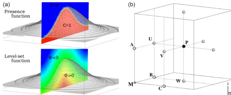
The numerical domain is divided into two regions: where the equations of continuum mechanics hold and a solid region embedding the obstacle where they do not. After comparing the methods (Fig. 1a) based on a local volume fraction func-tion and the LSF (Sussman et al., 1994; Kempe and Fröh-lich, 2012), it was decided to use the LSF as it was able to capture the interface between the fluid and solid regions more accurately. The|φ|distance informs us about the min-imal distance to the fluid–solid interface and theφsign about the region nature: sgn(φ) >0 for the solid one; otherwise, sgn(φ) <0. The vectornnormal to the interface and its lo-cal curvatureσ are defined asn= ∇φ

|∇φ| andσ= −∇ ·n.

Fig-ure 1a illustrates the continuous variation of LSF for an arbi-trary bell-shaped interface. The LSF is estimated at the seven available point types per cell to limit the discretization er-rors (Fig. 1b): at the mass pointP, where prognostic scalar variables are localized, at the three velocity nodesU, V , W where each projectionuis characterized, and at the A, B, C vorticity nodes employed by turbulent variables. The points of the solid region act as external points of the computational grid (as do external points in a boundary-fitted method at the grid limit). An intensive study has been done to estimate the modeling of the vector normal to the interface and the lo-cal curvature using LSF. The forcing based on a ghost-cell technique (GCT; and CCT or cut-cell technique) is applied to the explicit-in-time schemes (and the pressure solver) and detailed in Sect. 3.1 (and Sect. 3.2).

Figure 1. (a)Illustration of two ways to model a fluid–solid interface: the color code indicates the isocontours of the presence functionC

and the level-set functionφ.(b)Definition of the point types per cell:Mis the geometric mesh point,P the mass point,U, V , Wthe velocity nodes, and A, B, C the vorticity nodes.

the solid region. Expecting a correction due to IBM, wherein φ≥0, a general formulation of the tendencies is written as

∂ ∂t =

∂ ∂t

csl + ∂

∂t

ibm

. (10)

The right-hand-side (RHS) first term of Eq. (10) is given by the conservation laws (Sect. 2.1). The _∂t∂

ibmtendency is the correction due to the GCT in the solid region and near the immersed interface, satisfying the ψ desired boundary conditions atφ=0:

∂ψ ∂t

ibm

= −∂ψ ∂t

csl +ψ

n+1 −ψn

1t . (11)

Note that∂_∂tu

ibmis taken into account in the ERK temporal algorithm. The freeze of the immersed wind conditions in the ERK algorithm has also been implemented; it has shown more unstable behavior for a large Courant number.

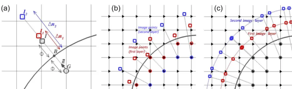
The forced points are called ghost points and are renamed ghosts. To estimate the variable ψ and for each ghost, the physical information is extracted near the interface and from the fluid region. The extension (grid stencil) of the forc-ing zone depends on the spatial accuracy of the numerical scheme. For example, Fig. 2b–c show the case of a two-layer stencil in a two-dimensional grid. The characteriza-tion of the layer is done by a condicharacteriza-tional loop applied di-rection by didi-rection on the LSF. For a 2-D case, the sign of φ (i, j )·φ (i,[j−kl:j+kl])andφ (i, j )·φ ([i−kl:i+kl], j )

is estimated. The integer valuekl determines the cells

trun-cated by the interface: kl=1 (kl=2) defines the first

(sec-ond) layer. The calculation of these ghost layers has a com-putational overhead due to data exchange among processors in parallel simulations. The stencil of the numerical scheme modeling the interface defines thekl value. In order to limit

this overhead, a low-order version of a centered explicit-in-time scheme (Sect. 2.1) is employed when φ >−1. The

CPU cost of the “hybrid” advection scheme is largely com-pensated for by the decrease in the ghost number and par-allel exchanges. Appendix B reports a comparison analy-sis between third-order weighted essentially non-oscillatory (WENO) and second-order centered schemes used in the vicinity of the interface; the studied case is the inviscid flow around a circular cylinder.

In classical GCT (Tseng and Ferziger, 2003) the fluid in-formation is obtained at a mirror point (noted I, renamed mirror) found in the normal direction to the interface in such a way that the interface nodeB is equidistant toI andG. Figure 2a shows the characterization of one ghostG(of LSF valueφG), its associated mirrorI (of LSF valueφI) and the

interface nodeB(GI =2φGn). Figure 2b illustrates several

ghosts and mirrors. The|I B|distance depends on the forc-ing stencil, and a problematic case regularly met in the mir-ror interpolation is the vicinity of ghosts with the interface (φG= −φI1, with 1the space step), leading to a not

well-posed condition.

The new GCT. To overcome this problem, we define

im-age points (notedI1andI2in Fig. 2a; renamed images) hav-ing a distance to the interface that depends only on the grid spacing:GIl=l1+φGnwithl=(1;2). Figure 2a shows

the images for one ghost. The new approach enforces a large enough value of the|IlB|distance. Figure 2b (c) illustrates

Figure 2. (a)Node definitions acting in the ghost-cell technique: the ghost (G), interface (B), normal vector (n), mirror (I) and images (I1, I2). (b,c) Illustration of classical (new) GCT using the mirror (images). Triangles correspond to one of the node types (see Fig. 1b).

build the Lagrangian interpolation: ψa(I )=

2La_G(I )ψ (B)+La_I

1(I )ψ (I1) +La_I

2(I )ψ (I2) 1+L a

G(I ) −1

, (12)

ψb(I )=Lb_B(I )ψ (B)+Lb_I

1(I )ψ (I1)+L b

I2(I )ψ (I2), (13) whereLa(I )andLb(I )are the Lagrangian polynomials, as follows.

La_I 1(I )=

21−φ

1

2φ 1+φ

La_I 2(I )=

_φ−1 1

2φ 21+φ

La_G(I )=

φ−1 φ+1

φ−21 φ+21

(14)

Lb_I 1(I )=

₂₁₋ φ 1 φ 1

Lb_I 2(I )=

_φ−1 1

φ 21

Lb_B(I )=

φ 1

φ−21 21

(15)

The accuracy of an interpolation depends on theψprofile. For example, a logarithmic evolution of the tangent veloc-ity is expected in LES. Otherwise, when the viscous layer is modeled, a linear evolution is expected. To compare the abil-ity of each quadratic interpolation to approach a wide vari-ety of profiles, the recovery of power laws such asψ=φ3/2 (Fig. 3a) and ψ=φ1/4 (Fig. 3b) is studied. As illustrated, PLIafits the two analytical solutions better and is therefore adopted. The classical and new GCTs have been compared thoroughly, and part of this analysis is deferred to the Ap-pendix. The interpolated field of the potential flow around a single cylinder or a sphere was compared to the theoretical solution; the sensitivity of the inviscid flow around the same

bodies (Appendix B) to the type of GCTs has been stud-ied. The new GCT has given the best results, especially in the symmetry preservation in the inviscid flow cases. Note that these results are also dependent on the 3-D interpola-tion choice detailed in the following paragraph. The proposed GCT is employed in the rest of this study. The GCT imple-mentation is divided into four main steps: the fluid informa-tion recovery, the interface basis change, the interface condi-tion and the ghost value.

The fluid information recovery.ψ_Il, for the images con-tained in a pure fluid cell (all corner nodes are in the fluid region), is recovered by a trilinear interpolation based on La-grangian polynomials (LP), as follows.

LLP_i (xl)= N Y

p=1,p6=i

xl−xp

xi−xp

LLP_j (yl)= N Y

p=1,p6=j

yl−yp

yj−yp

LLP_k (zl)= N Y

p=1,p6=k

zl−zp

zk−zp

(16)

ψ (xl, yl, zl)= N X i=1 N X j=1 N X k=1

LLP_i (xl)LLPj (yl)LLPk (zl)

·ψ (xi, yj, zk) (17)

For truncated cells (at least one corner node is in the solid region),ψ_I

l is recovered using an inverse distance-weighting (DW) interpolation:

ψ (xl)= N P

i=1

LDW_i (xl).ψ (xi) N

P

i=1

LDW_i (xl)

;

|xl−xi|=

q

Figure 3.Quadratic interpolations of two analytical profilesψ=φn(red lines) using two image points atφ= −[1;2]1and the interface node. Green (blue) corresponds toLa(Lb) polynomial results.

where LDW_i (x)=|xl−xi|−α (α=1). This formulation

di-verges when xi→xl and it is commonly adopted to

impose ψ (xl)=ψ (xi) when ∃(xi−xl)≤ ( is an

ar-bitrary parameter depending on the mesh discretization, 1). The 3-D extension is direct with |xl−xi|=

p

(xl−xi)2+(yl−yi)2+(zl−zi)2. The use of these

inter-polations was decided after comparisons with barycentric Lagrangian and modified distance-weighting interpolations (Franke, 1982) and tests on theαcoefficient. As the bound-ary condition is expressed in the interface frame and the grid is staggered, the non-collocation of the ucomponents im-plies the interpolation of three different classes of cells (with U, V , W corners; Fig. 1b) for eachU, V , Wghost and build-ing the change of frame matrix for which the proposed GCT presents an interest during the characterization of the direc-tion tangent to the interface.

The interface basis change. Velocity vector u, known in

the Cartesian mesh basis at the images Il (1n1=1 and

1n2=21 in Fig. 2a), is projected in the basis of the in-terface(n(B),t(B),c(B))in which the boundary conditions on each vector component are imposed. Computing the LSF gradient, the normal direction is defined. Otherwise, (t,c) represents two arbitrary tangent directions. The tangent di-rection tis considered the predominant tangent direction of the flow along the fluid–solid interface depending on the image values and defining the velocity vector as u(Il)=

un(Il)n+ut(Il)t(Il). The cotangent direction is defined as

c(Il)=

n⊗u(Il)

||n⊗u(Il)||

; t(Il)=c(Il)⊗n. (19)

The(n,t,c)basis at the interface is defined by considering (or not) the rotation of the tangent velocity with the distance to the interface:

t(B)=t(I1) if no rotation;

et(B)=2et(I1)−et(I2) if linear evolution. (20)

Finally, the third component isc(B)=n⊗et(B)and

(in-verse) projection is known.

The interface condition. Let ψ_B and 1∂ψ_∂nB be the

Dirichlet and Neumann conditions on ψ. The general for-mulation of the boundary condition ψ (φ=0) is written as a Robin condition:ψ (φ=0)=krψB+(1−kr).(ψ (φ=

−l1)−l1∂ψ_∂n

B). The switch between the Dirichlet condition

and the Neumann condition is done through the coefficient kr∈ [0:1]. To give some examples of a Dirichlet condition, (kr;ψB)=(1;0)is imposed on theu·nvelocity component

normal to the interface arising from the impermeability hy-pothesis and on theu·tcomponent tangent to the interface for a no-slip hypothesis. To give some examples of the Neumann condition imposed by(kr;∂ψ_∂n

_B)=(0;0): a no-flux condi-tion on the potential temperature (as well on a passive scalar, subgrid kinetic energy) and a free-slip case applied tou·t. Note the lφ₂ approximation in the location of the derivative term and the Neumann condition depending on the chosen image (in practice the selected imageIl is the closest one to

the interface).

An interface condition depending on the characteristics of the surrounding fluid such asψ (φ=0)=F (ψIl;

∂ψ ∂n

Il)is a wall model. Using two (three) images, simple wall models such as the constant (linear) extrapolation of theψgradient is reached by the ∂2ψ

∂n2 Il

=0 (∂3ψ

∂n3 Il

=0) computation. The consistency between the tangent component to the interface of the resolved wind and the subgrid turbulence is the subject of Sect. 2.3.

The ghost value. Knowing ψ (φ=0) and ψ_Il=ψ (φ=

as

ψ (G)=2ψ (B)−ψ (I ) (Dirichlet), ψ (G)=2φdψ

dn _B

+ψ (I ) (Neumann). (21)

In practice, three Il images are defined for which the

lo-cations are φIl = −l1 with l= [1/2;1;2]. The choice of the image distance to the interface affects the results. To best approach the expected solution, two quadratic interpo-lations depending on the images used and one combination of these quadratic interpolations are tested. Figure 4a and b illustrate these interpolations by considering two analytical profiles (red lines): the quadratic interpolationQI1(QI2) is based on the image values located atφ=1/21andφ=1 and plotted in green symbols (at φ=1 andφ=21 plot-ted in blue symbols). Depending on the analytical profile, Fig. 4 shows the influence of the image location choice. As expected, QI1 (QI2) appears to be less accurate than QI2 (QI1) forψ (φ∈ [−21: −1])(for ψ (φ∈ [−1:0])). QIC is the combination ofQI1andQI2(purple line).QIC

preserves the advantage of each quadratic interpolation and when φG< 1 (φG> 1),QI1 (QI2) is used in the rest of

the study. Knowingψn+1(φ−)at the end of the MNH tem-poral loop with QIC, theψ

n+1

(φ+)profile is extrapolated from the fluid region to the solid region by applying an anti-symmetry ψn+1(φ+)=2ψn+1(0)−ψn+1(φ−). The ghost value is estimated and theψgradient at the interface is also recovered.

3.2 Cut-cell technique and pressure solver First looking at the RHS of Eq. (5), the ∂(ρru∗)

∂t

_csl coming from the resolution of the explicit-in-time schemes near the interface and in the solid regions badly affects the ∇ ·u∗ computation (note that the GCT operates after the step pro-jection). Therefore, the fictive wind of the solid region can spread errors in the fluid region during the pressure resolu-tion. To avoid it, a correction of the pressure solver is pro-posed.

The elliptic problem (Eq. 5) is rewritten as a resolution of the linear systemP·9∗=Q. In the standard MNH version, ∇ ·u∗=Qis estimated using a finite-difference approach. To uncouple the solid region from the fluid region our revisited version enforces a null divergence for pure solid cells and estimates the balance of momentum fluxes by a finite-volume approach for truncated cells (notedQcct):

V∇ ·u∗= Z

Vf

∇ ·u∗dV+ Z

Vs

∇u∗dV=X±ui∗·Si

=X±^₁2_u

i∗, (22)

whereV=13is the cell volume,Vf(Vs) the fluid (solid) part ofVandSithe cell surfaces for whichiis the index of each

surface orientation [e, w, n, s, b, f] as illustrated in Fig. 5a. According to the Green–Ostrogradski theorem, theui∗Si

calculation is the classical way of a CCT (Yang et al., 1997; Kim et al., 2001) to estimate the velocity divergence. A sim-ilar approach is performed here by rebuilding the flux₁]2_u∗

for truncated and solid cells. The±1^2_u

i∗calculation consists of a weighting of the

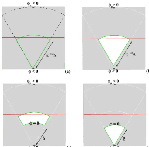
out-flux and inout-flux function of the fluid and cell surface ratios (Fig. 5a). Figure 5b gives an example of the west surface (i=w, red border) in which₁^2_uw∗

(j, k)is calculated us-ing the LSF valueφ=φwand the ones of the eight adjacent nodesφp(j±1, k±1). A disk of radius −1

√

π 1is split into eight “piece-of-cake” segmentsP_p∗(p= [1:8]). An LSF lin-ear interpolation detects (or not) the interface location. In the presence of an interface, its distance from the studied node is 0< δp< −1

√

π 1. Knowingδp, the momentum flux balance

is formulated for a nonmoving body as (pis the index of the piece of cake andithe index of the cell surface)

^ 12_u

i∗=

12 8

" ₈ X

p=1

H(−φp)H(−φi)ui∗

+ 8 X

p=1

H(−φpφi)· |H(−φp)−π _δ

p

1 2

|

·H(−φp)up∗+H(−φi)ui∗ i

. (23)

The four encountered cases correspond to a pure fluid cell ^

12_u

i∗=1 2 8

8 P

p=1

ui∗whenφp<0 andφi<0 (Fig. 6a); a pure

solid cell₁^2_u

i∗=0 whenφp>0 andφi>0 (Fig. 6b); and

two types of truncated cells depending on the fluid–solid na-ture of the main node for whichφp.φi<0 (Fig. 6c–d). Using

Eq. (23), Eq. (22) is solved and leads to the RHS computation of Eq. (5).

Figure 4.Profile normal to the interface of two points of fluid informationψ: analytical solution (red lines), quadratic interpolationQI1

usingψ_−φ=[1/2;1]1(green symbols),QI2usingψ−φ=[1;2]1(blue symbols),QICas a combination ofQI1andQI2(purple lines).

Figure 5. (a) Momentum flux balance for an arbitrary truncated cell of volume V, where the ui∗ velocities (Ui in the figure, i= [e, w, n, s, b, f]) are supported by theSi surfaces in grey; the transparent volume is a part of the solid body.(b) Segmentation of the Swarbitrary surface (red border) in eightPp∗pieces of cake (the border ofP3∗is indicated in green).

M P

m=1

P−1_.Qm

cct, where M is the number of iterations. This number is limited by a convergence criterion (compromise between incompressibility satisfaction and CPU cost). Many iterative procedures are available in MNH originally devel-oped for non-Cartesian grids. Richardson and preconditioned conjugate residual algorithms have been adapted here to the obstacle immersion. The newly modified pressure solver is tested and validated in Sect. 4.1.

3.3 Consistency with the turbulence scheme It is known that lm

l →1 is a reasonable approximation in nonhomogeneous, non-isotropic turbulence such as in the near-wall region. This approximation is indeed retained in the present IBM implementation, which assumes lm=l

(hereafter notedlm and called the mixing length). The

Re-delsperger et al. (2001) corrections near the ground are to

match the similarity laws and the free-stream model con-stants are not activated. lm is equal to the numerical

cut-off space scale sufficiently far from the ground, leading to a1√eturbulent viscosity. Near the ground and following the Prandtl idea consisting of the assumption of the linear variation oflmin the near-wall region, the upper limit of the

mixing length is min(kz, 1)(kis the von Kármán constant andzis the altitude).

The turbulent characteristics are highly affected by surface interaction. As a consequence and for LES, the subgrid tur-bulence scheme (Sect. 2.3) is modified in the presence of immersed obstacles in the subgrid turbulent kinetic energy equation (Eq. 6), mixing length computation and Reynolds stress diagnosis (Eqs. 7, 8 and 9).

The subgrid turbulent kinetic energy condition. The

Figure 6. (a–d) ±1^2_u

i∗ calculations depending on the signs of

φi=(φ)and φp on an arbitrary piece of cake. The white (grey) region corresponds to the solid (fluid) one ofP_p∗(same color code as in Fig. 5).

STKE profile is considered parabolically in the viscous sub-layer (Craft et al., 2002; Bredberg, 2000) and constant in the inertial and wake outer layers (Kalitzin et al., 2005; Capiz-zano, 2011). Due to the high turbulent Reynolds number

Ret≈O(104−105)encountered, a homogeneous Neumann condition is applied at the immersed interface. The equilib-rium between the production and dissipation of STKE could be discussed and controverted; this choice acts as a first stage in IBM development.

The near-wall correction of the mixing length. The von

Kármán limitation due to immersed walls acts through the LSF, and the upper limit on the mixing length lm near the

interface becomes min(kz,−φ, 1) with a banning of neg-ative values in the solid region. Whatever the production of STKE and the turbulent shear, the lower limit lm(−φ≤

0) induces a null value of the diagnosed surface fluxes. In addition, a singularity appears in the dissipative term ρrKe3/2lm−1. Through pragmatic reasoning, the singularity

due to l_m−1(φ→0−)→ ∞ amounts to the modeled length scales being smaller than the Kolmogorov scale (ν3−1)14. Considering the Kolmogorov scale as modeled, the turbu-lence should vanish, which is in contradiction to the dis-sipative term. In order to overcome this ill-posed problem, a lm lower limit has to be specified. In the study of

atmo-spheric flows around buildings, a characteristic thickness of the viscous layerH /

√

Recan be defined around anH bluff body for a Reynolds number based on the obstacle scale: H≈O(10m);Re≈O(107). This thickness estimate is also

Figure 7.Illustration of the unresolved physical processes near a nonidealized solid wall (black line) in an atmospheric context: the length scale based on the viscous effects (grey line) is drastically smaller than the roughness length. The roughness length approaches the scale of smallest eddies and governs the log-law profile.

proportional to Eν/u∗ (E≈9.8 is commonly employed), whereby the friction velocityu∗ is about 1 cm per second. Following these estimates, the length scale due to the vis-cous effectsz_νibbelongs to the millimeter domain in the ex-pected atmospheric cases. Looking after a building surface and its large heterogeneity (door, windows, surface charac-teristics), its roughness lengthzib₀ is at least in the decime-ter domain andzib₀ > zib_ν (Illustration in Fig. 7). For lowRe

and smooth surfaces,zib_ν > zib₀ could be encountered. There-fore, we assumezib=max(z₀ib, z_νib)and thatzibis related to the size of smallest unresolved eddies near walls (i.e., dissi-pative scale). The mixing length near the wall iszib< lm<

min(kz,−φ, 1).

The turbulent fluxes correction. Theψ gradient and the

turbulent diffusionO(zib√e)prescribe the turbulent fluxes at the immersed interfaces (Eqs. 7, 8 and 9). As a first step in the MNH–IBM implementation, a no-flux condition on the mean potential temperature is imposed, leading to a zero value of the sensible heat flux. Writing the mean velocity field at B as u=utt, ut(B) is needed to recover a

gra-dient consistent with the turbulent shear. Considering the Prandtl (1925) or von Kármán (1930) theories, the logarith-mic profile is assumed in the vicinity of the wall accord-ing tout(z)=u

∗

k ln

1+ z

zib

. Considering1to be the limit of the resolved scales, most of the turbulent kinetic energy 1

2(u

02_+v02_+w02_{)is contained in the subgrid when−φ < 1} and asKtke√ewith a constantKtke_&1. This assumption is reinforced by the homogeneous Neumann condition applied one. This approach derives from RANS (Reynolds-averaged Navier–Stokes) approaches, and the velocity friction is for-mulated asu∗=Ktkep4

Cµ

√

e, whereCµis a constant

establishes an equilibrium between the production of STKE and the mean parietal friction. Note that the use of a log-law model near a singularity such as sharp edges and cor-ners could be called into question. Nevertheless, Section 5.1 and 5.2 show LES results employing this proposition. After numerical investigations done during the single-cube study, Ktkep4Cµ≈1 appears to be a suitable choice.

4 Flows around a circular cylinder 4.1 Potential flow

Isolated from the rest of the code, the resolution of the pseudo-Poisson Eq. (5) leads to potential solutions (Sect. 2.2). Theoretical ones are available for flow developed around a nondeformable obstacle such as an infinite cylinder or a sphere (Milne-Thomson, 1968; Batchelor, 2000). The two bodies are investigated here. The flow around the infi-nite cylinder is predominantly presented.

Figure 8 illustrates the cylinder case. The fluid density is considered constant in time and in space. The flow is initially imposed as spatially homogeneous with a constant module of velocity U∞ and parallel streamlines (Fig. 8a).

This initialization does not respect the conservation of the momentum flux, and the irrotational correction of the pro-jection method goes to recover this conservation. At the same time, the impermeability of the cylinder of diameter Dcyl=2Rcyl is achieved. Figure 8b shows the streamlines obtained with the MNH pressure solver modified to take into account the presence of immersed obstacles (Sect. 3.2). Defining x as the direction parallel to the initial stream-lines and yas the perpendicular one, the expected solution is u·U∞−1=cosα(1−

R2 cyl

r2 )x−sinα(1+ R2

cyl

r2 )y (single and non-confined body,(α;r)cylindrical coordinates). The nu-merical confinement is discussed hereafter, characterized by L=Lcyl/Rcyl, whereLcylis the distance separating the lat-eral domain surfaces (Fig. 8a).

The Richardson (RICH) and the residual conjugate gra-dient iterative (RESI) methods are tested (Sect. 3.2). Fig-ure 9a plots the evolution of the dimensionless residue

16);0.14 %(N=32)] in regard to the incoming flux local-ized by itsxinletlongitudinal coordinate. Similar results were obtained with a spherical body (not shown here).

With a change of Galilean reference frame, this study cor-responds to a uniform body accelerationabin a fluid initially at rest. However, a possible viscous term, the hydrodynamic force exerted on the body, is reduced to the added mass effect

Amfab= R

Vs ∂ρfu

∂t dVfor1t→0.Ais the dimensionless

co-efficient andmfthe displaced fluid mass.Acyltheoretically equals 1 in the non-confined cylinder case (Lamb, 1932). The red curve in Fig. 9b illustrates the effect of the confinement L on Acyl for N =16 resolution. Unsurprisingly, Acyl in-creases with the confinement (Brennen, 1982). The weak de-pendence ofAcylwithL >16 allows us to consider the body to be isolated forL∼16. The green curve in Fig. 9b shows the impact of the space resolution forL=16. The numer-ical added mass coefficient is in good agreement with the theoretical one, presenting a relative error of about 2 % for N >16. It induces a respect for the impermeability hypoth-esis at the immersed interface. A similar study for a spher-ical body givesAsph=1₂+0.4 %. Figure 10 illustrates the contours of the kinetic energy around the sphere in an arbi-trary symmetry plane. The green contours (numerical solu-tions) fit well with the red contours (theoretical solusolu-tions). A convergence study of the pressure solver is discussed in Appendix A.

4.2 Viscous flow

A pure dynamic and well-documented case that naturally follows previous ones is studied here. This physical case is the wake past a circular cylinder (non-stratified flow) at two moderate Reynolds numbersRe=(40;140). One of the fore-runners is Taneda (1956), who experimentally studied the na-ture of eddy strucna-tures.

Taneda (1956) found a regular Hopf bifurcation at a crit-ical Reynolds number Rec=

U∞Dcyl

11-Figure 8.Potential flow around a cylinder:(a)initial state around the body of diameterDcyl=2Rcyl;(b)streamlines obtained after the

Poisson equation resolution. The confinement is defined asL=Lcyl/Rcyl).

Figure 9.Potential flow around a cylinder:(a)velocity convergence of two iterative methods (residual conjugate gradient, Richardson) for different spatial resolutionsN= [4:32](L=16);(b)evolution of the added mass coefficientA(N;L)with the confinementL=Lcyl/Rcyl

(N=16) and with the node number per radius cylinderN(L=16). The confinement is defined in Fig. 9a.

Figure 10.Potential solution around a sphere:(a)kinetic energy in an arbitrary symmetry plane;(b)zoom.

d). The standing eddy (the von Kármán street) obtained by MNH–IBM atRe=40 (140) is visualized in Fig. 11a (b) by the injection of a passive tracer on the body surface.

The standing eddies atRe<Recare commonly described with aθddetachment angle,lrrecirculating length and(a;b) location of the vortex core (Fig. 12). The limit of the numer-ical domain is 10Dcylupstream of the obstacle for the inlet condition (U∞, the uniform incoming velocity) and lateral

condition (slip condition) and 15Dcylfor the outlet condition, allowing for the vorticity evacuation. As Cai et al. (2017) mention, this domain can induce a low numerical confine-ment effect. Three regular Cartesian meshes are built with 10, 20 and 30 nodes perDcyl.

Figure 11.Eddy structure in a viscous fluid: steady (left,Re≈40) and unsteady (right,Re≈140) solutions obtained by the current numerical investigation (aandb, MNH–IBM and 30pts/Dcyl) and by the Taneda (1956) experiments (candd). The visualization is due to the presence

of a passive tracer injected on the body surface and transported by the flow.

Figure 12. Recirculating region at Re=40 (MNH–IBM, 20pts/D_cyl): definition of the θ_d (◦) separation angle, lr

recir-culating length and (a;b) vortex core location. The distance is dimensionless byDcyl.

The 10pts/Dcylmesh shows more discrepancies, which are attributable to the nonability of the coarsest resolution to capture the viscous boundary layer for which the thickness evolves inDcyl−1

√

Re. Note that the impact of the low-order (centered or WENO) modeling of the advection at the im-mersed interface is weak for this viscous case (Sect. 3.1). Table 1 compares the 20pts/Dcyl results with a part of the results literature collected in Gautier et al. (2013).

The focus is on the unsteady mode atRe=140. The ratio between the characteristic time of inertial effects Dcyl/U∞

and the one related to the vortex shedding 1/f defines the Strouhal number St=f D

U∞. Brazza et al. (1986), Park et al. (1998) and Stålberg et al. (2006) confirm the equa-tionSt(Re)= −3.3265/Re+0.1816+1.6·10−4/Reproposed by Williamson (1989). MNH–IBM obtains St(Re=140)∈ [0.177:0.179] and an absolute maximum relative error

Table 1.Description of the standing eddies in the wake of the solid cylinder (Re=40): comparison of the separation angleθd(◦),

re-circulating lengthlr(m) and vortex core location(a;b)between the literature and MNH–IBM.

Authors θ_d(◦) lr/Dcyl b/Dcyl a/Dcyl Coutanceau and Bouard (1977) 53.8 2.13 0.76 0.59 Linnick and Fasel (2005) 53.6 2.28 0.72 0.60 Taira and Colonius (2007) 53.7 2.30 0.73 0.60 Bouchon et al. (2012) 53.4 2.26 0.71 0.60 Gautier et al. (2013) 53.6 2.24 0.71 0.59 Cai et al. (2017) 54.5 2.34 0.76 0.62 MNH–IBM 30pts/Dcyl ≈54 ≈2.2 ≈0.7 ≈0.6

lower than 2 % in regard to the Williamson (1989) formu-lation with the two finer resolutions. Our results are in good agreement with those presented in the abovementioned and more extensive studies. Details on DNS validation in a vis-cous buoyancy-driven flow are also presented in the Supple-ment.

5 Turbulent flows around parallelepiped(s)

Common hypothesis and methods.The fluid is considered as neutrally stratified. The Coriolis term is negligible due to the addressed space scales and timescales. The turbulent diffusion is modeled by the subgrid TKE1.5 scheme trans-ported by PPM (Sect. 2.3). All surfaces are considered non-permeable and the IBM wall model (Sect. 3.3) is activated. An(x, y, z)reference frame is defined (z, vertical direction) and the velocity vector is written asu(t)=u(t )x+v(t )y+ w(t )z. A time simulation is needed afterwards to establish the turbulence state (not shown here). The overline notation refers to the mean value in time in this section.

5.1 Flow over a surface-mounted cube

Using static pressure measurements, as well as laser-sheet and oil-film visualizations, Martinuzzi and Tropea (1993) and Hussein and Martinuzzi (1996) generated a large data set for the study of flows around a cubic body placed in a channel (Fig. 13a). RANS and LES have been used to ex-plore in detail this physical case (Breuer et al., 1996; Shah and Ferziger, 1997; Rodi et al., 1997; Frank, 1999; Krajnovic and Davidson, 2002; Farhadi and Rahnama, 2006).

Physical details. A cube (H side) is placed in a channel

of 2H height. The channel is sufficiently large in the span-wise direction to consider the cube to be single in that di-rection. Turbulent flow is generated in the channel upstream of the cube with a mean bulk velocityUb. Defining the di-mensionless wall coordinatez+=u∗·z/νf, the stream-wise upstream velocity corresponds to a log law for smooth walls u(z+)·u∗−1=5.54+1

κlog(z

+_{)as described in Hussein and}

Martinuzzi (1996). The Reynolds number, as defined by the mean bulk velocity, the cube height and the molecular diffu-sion, isRe≈40 000.

The mean flow around the cube presents a set of five re-circulating regions (Fig. 13b). Each cube surface is associ-ated with one of these regions: the A–B vortex separations in front of the cube, which spread laterally in a horseshoeD, two vortices near side wallsE, oneF on the roof and main arch vortexGdownstream.

Numerical details. The top and bottom surfaces of the

cubic body are modeled by the IBM. A small value of the roughness length z0/H≈10−6 is imposed (low value to model a smooth interface, viscous-scale intervention in the z+ calculation). The stream-wise (spanwise) direction is x (y). The size of the grid is set as (x, y, z)=(−24H: 8H,−4H:4H,0H:2H )with a location of the cube center at(H₂;H

2;

H

2). Three regular Cartesian meshes are employed with a respective space step H /1= [10;20;40]. x/H ∈ [−24: −4]is a region employed to model the fully turbu-lent character of the incoming flow. The incoming turbuturbu-lent state is obtained by the IBM and a pseudo-recycling method inspired from the works of Lund (1998), Mayor et al. (2002), and Yang and Meneveau (2016) (not detailed here). The ver-tical profiles of the stream-wise velocity and turbulent inten-sitypu02_/U2

b≈2.10

−2_{(Hussein and Martinuzzi, 1996) are}

recovered atx/H∼ −4. We note that the turbulence gener-ation deserves more attention, but we prefer to concentrate only on the cube wake.

Results. Figure 14a, b and c show the time-averaged

streamlines in the vertical symmetry plane of the cube ob-tained by MNH–IBM for the three space resolutions. The streamlines of the coarse, medium and fine resolution are respectively in red, green and blue. The discretization or-der of the fine resolution is close to that of most literature LESs except Shah and Ferziger (1997), who used a far more precise grid near walls. The same figure obtained by the ex-perimental investigation is given in Fig. 14d. The size of the front (rear) region is characterized by the recirculating length xf/H (xr/H). The experiment gives xf/H≈ [1.04:1.05] andxr/H≈ [1.64:1.67]. The LES reference results give the ranges xf/H∈ [0.81:1.28] and xr/H∈ [1.38:2.25]. For the two finest resolutions (green and blue), the overall pre-diction of MNH–IBM recovers a consistent mean topologi-cal structure. MNH–IBM obtains for the two finest resolu-tionsxf/H∈ [0.99:1.21]andxr/H∈ [1.48:1.55]. MNH– IBM does not capture, as with most LESs, the two divid-ing linesA/B mentioned by Martinuzzi and Tropea (1993) but only captures a flattened vortex. However, the bifurcation point near the rear edge and ground is not detected by MNH– IBM, while this point was modeled in Rodi et al. (1997). This bifurcation point was also commented on in Martinuzzi and Tropea (1993), even if their experimental uncertainty did not allow us to visualize it in Fig. 14d.

Figure 14e shows an MNH–IBM instantaneous flow field with the Q criterion (Hunt et al., 1988), and as the LES ref-erence results mention, it presents a highly intermittent char-acter clearly visible with the quasi-disappearance of theD horseshoe and G arch. A frequency f of vortex shedding dominates the highly intermittent activity in the body wake, leading to the experimental Strouhal number St=f·H

Ub ≈ 0.145. An MNH–IBM energy spectrum (discrete Fourier transform ofw(t )in the body wake) finds a peakSt∈ [0.10: 0.12]for all the studied resolutions and a∼ −5/3 energetic cascade slope for larger wave numbers (not shown). TheSt

values obtained by MNH–IBM are slightly lower than the ex-perimental one but stay consistent with theSt∈ [0.10:0.15] range of other LESs.

Still in the vertical symmetry plane of the mean flow, Fig. 15 plots at four longitudinal positions x/H= (1/2;1;2;4)the vertical profiles of time-averaged quantities related to the steady (u,w) and unsteady (TKE,u0_w0_{) parts of}

vortex structure around a cube (Martinuzzi and Tropea, 1993) and index of the recirculating regions.

Figure 14.Vertical symmetry plane of the mean flow:(a–c)MNH–IBM time-averaged streamlines;(d)streamlines observed by Martinuzzi and Tropea (1993);(e)MNH–IBM instantaneous visualization of the Q criterion (Hunt et al., 1988).

existence of the bifurcation pointS1 (Fig. 15b). An underes-timation appears on the counterflow at(x/H;z/H )≈(2;0) and is frequently observed in the literature (Fig. 15c). Some discrepancies are found on twowprofiles (Fig. 15f–g). Note that Shah and Ferziger (1997) and Krajnovic and Davidson (2002) highlight the difficulty of recovering it. The turbulent kinetic energy and the Reynolds stress are correctly predicted at the cube roof (Fig. 15i–j). The vertical profiles of TKE and u0_w0_{downstream of the cube show an overestimate tendency}

(Fig. 15k, p, l). No experimental data are available on TKE at x/H =4 (Fig. 15l), but using theu02_(x/H=4) experimen-tal value (not shown here) and theu02_{/TKE ratio obtained by} MNH–IBM, we suspect that TKE(x/H=4)is still

overesti-mated. This turbulence diagnosis is relatively similar to that of Farhadi and Rahnama (2006).

Sensitivity study.Some tests have shown a sensitivity of

con-Figure 15. Mean vertical profiles of velocities (top), turbulent kinetic energy and Reynolds stress (bottom). The lines correspond to the MNH–IBM results. The symbols are the Martinuzzi and Tropea (1993) data except for TKE (Hussein and Martinuzzi, 1996). The profiles are given at four longitudinal locations:(a, e, i, m)x/H=1/2;(b, f, j, n)x/H=1;(c, g, k, o)x/H=2;(d, h, l, p)x/H=4.

dition. Theu∗−√1_e=K tke1/4

√

Cµratio and thez0roughness length fixed in the immersed wall model (Sect. 3.3) impact the nature of the incoming turbulent state for which the sur-face shear plays an important role. To give a significant ex-ample and if a null value ofKtkeis applied on the channel sur-faces (non-slip condition),xfhighly increases and the vortex

atS2 appears. Otherwise,Ktkeandz0do not crucially affect the nature of the dynamic in the vicinity of the cube surfaces; the pressure gradient between front and back faces governs.

main interest lies in the similitude between this experiment and a pollution episode due to toxic gas propagation over a city with high population densities. It provides extensive measurements of meteorological variables and scalar disper-sion information.

Physical details. The near-regular array is composed of

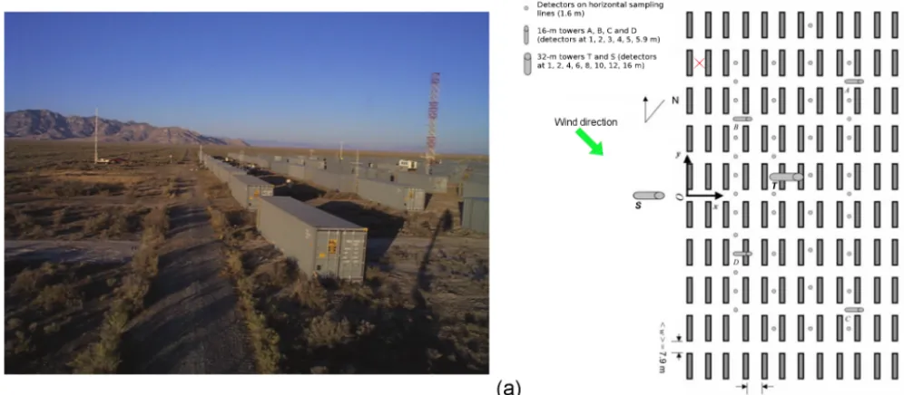
120 containers. Figure 16 gives a photograph and a picture of the topography. The containers are equivalent in volume and shape. Their spatial dimensions are (Lx, Ly, Lz)=∼

(2.4,12.2,2.5)m and the horizontal distance between con-tainers is O(10)m. Following Table II in Yee and Biltoft (2004), the 2681829 case (25 September 2001 at 18:29 UTC) is selected. The Monin–Obukhov length is Lmo≈28 000 m and the stability condition is supposed neutral; the buoyancy effects and the sensible heat flux are negligible in regard to the inertia effects and the turbulent shear. The incoming flow shows a mean horizontal angle with the container lay-out (green arrow, Fig. 16b). The MNH–IBM results are com-pared to the experimental measurements reachable at several altitudes (4, 8, 16 m) at the south tower and at the main T tower placed in the array center. The locations of the towers are indicated in Fig. 16b. A roughness lengthz0=0.045 m is given by the experiment and related to the surrounding desert vegetation.

Numerical details. The externalized scheme SURFEX

(Masson et al., 2013) models the ground friction. LSF is gen-erated to represent the topography and IBM is used to model the containers. The smallest characteristic container length is discretized byO(10)cells. The mesh is a Cartesian and reg-ular grid forz <10 m with a space step1=0.2 m. Above 10 m, the vertical space step is released in a geometric pro-gression of 1.08 ratio. The altitude of the numerical domain top is about 8 times the container height.

The distance between the horizontal limit of the computa-tional domain and the array is about 20 times the container height. The large-scale flow is forced by an open boundary condition. A mean horizontal angle of−41◦with thex di-rection is fixed for all altitudes; note that the low angle devi-ation and the turbulence observed upstream of the containers in the experiment are not numerically considered. Following the experimental data given at the S tower (Fig. 17a, blue

canopy induces a global slowdown of|u|near the ground and up toz.8 m. A decrease in the mean horizontal wind angle is found at the same altitudes. This deviation is related to the container orientation, which tends toward the flow being aligned with they direction. The same pattern is discussed in Milliez and Carissimo (2007). A wind acceleration and an increase in the wind angle are observed by MNH–IBM forz_&8 m as in the LES results of König (2014) and Dejoan et al. (2010) on similar MUST cases. These few degrees of deviation are observed by the experiment but not the accel-eration. A part of this acceleration may be explained by a Venturi effect and a too-closed top limit of the computational domain (numerical confinement, under investigation).

Figure 18a (b) illustrates the time-averaged horizontal wind field|u|(|u| att=200 s) at the 1.6 m altitude. These figures highlight the fact that the incoming flow is not tur-bulent in the simulation. This assumed gap constitutes a per-spective (Camelli et al., 2005) not directly linked to IBM. It also allows us to introduce here some comments on the turbu-lence state. The atmospheric turbuturbu-lence is dependent on the roughness length (z0 considered constant due to the homo-geneous and flat desert over a few miles upstream). The first container rows are the scene of the boundary layer transition and act as a region of strong roughness change. The turbu-lence observed in the urban-like canopy has two origins: the incoming turbulence and that induced by the container pres-ence. The contribution of both turbulence types varies as a function of the altitude and distance to the first row.

The mean kinetic energyEk=1 2(u

2_+v2_+w2_{), friction} velocityu∗= 4

q

u0_w02_+v0_w02 _{and turbulent kinetic energy}

TKE=1 2(u0

nu-Figure 16. (a)Photograph of the MUST containers in Utah’s West Desert;(b)schematic representation of the container layout. The locations of the concentration (detectors) and wind sensors (S and T towers) are indicated, as are the position (red cross) of the pollutant release and the direction of the incoming flow (green arrow) for case 2681829. Source: Biltoft (2001) and Yee and Biltoft (2004).

Figure 17.Mean vertical profiles in the MUST experiment:(a)|u|horizontal velocity;(b)atan(v/u)wind direction at the S (blue) and T (black) towers. The symbols (lines) are the Yee and Biltoft (2004) experimental measurements (MNH–IBM results).

merical results. The experimental measurement of the fric-tion velocity atz=16 m is close to the upstream value.

The discrete Fourier transform of theutemporal evolution (Fig. 19) atz(T)=(4;8)m shows the coherence between the energetic cascade of the experimental investigations and that of the numerical ones. Atz(T)=16 m, MNH–IBM underes-timates the unsteady part of the solution for all wave num-bers. The same behavior is observed onvandw(not shown here).

The MNH–IBM results are consistent with the experimen-tal observations below z(T)_.10 m. This modeling induces the turbulence to be mostly due to the container wakes

up-stream of the T tower and not to the incoming turbulence (not modeled in the simulation). The influence of the atmo-spheric turbulence grows with altitude and MNH–IBM di-verges with the experiment. This divergence forz(T)_&10 m leads us to think that the thickness of the container has an in-fluence about 4–5 times the height of the urban-like canopy.

6 Conclusions and perspectives

Figure 18.Wind at the horizontal cut atz=1.6 m:(a)time-averaged on 200 s;(b)instantaneous att=200 s. The black squares indicate the location of the T and S towers (MNH–IBM results).

Table 2.Kinetic energy, turbulent kinetic energy and friction velocity obtained by the experimental (Yee and Biltoft, 2004) and numerical (MNH–IBM) investigations at three altitudes of the tower T.

Ek(m2s2) TKE (m2s2) u∗(m s−1)

MNH–IBM Yee and Biltoft (2004) MNH–IBM Yee and Biltoft (2004) MNH–IBM Yee and Biltoft (2004)

z=4 m 15.3 14.1 3.33 3.78 1.14 1.08

z=8 m 36.7 29.7 1.70 3.28 0.68 0.83

z=16 m 65.8 48.5 0.02 1.75 0.02 0.60

written for structured grids. The MNH–IBM aim is to explic-itly model the fluid–solid interaction in the surface boundary layer developed over grounds presenting complex topogra-phies such as cities or industrial sites.

A level-set function (Sussman et al., 1994) characterizes the geometric properties of the fluid–solid interface. Two original approaches of the ghost-cell (Tseng and Ferziger, 2003) and cut-cell techniques (Udaykumar and Shyy, 1995) are implemented to correct the MNH numerical schemes. A newly proposed GCT recovers the fluid information in sev-eral image points by presenting a distance to the interface in-dependent of the ghost’s distance. The CCT consists of a new finite-volume approach of flux balance near the immersed in-terface. The GCT is applied to the numerical schemes based on explicit time integration and the CCT is employed in the implicit resolution of the Poisson equation, satisfying the incompressibility hypothesis. The adaptation and use of it-erative procedures solves the pressure problem without any modification to the inverted matrix. The turbulence problem is closed at the fluid–solid interface by a pragmatic LES– RANS formulation based on the subgrid turbulent kinetic en-ergy and the length of the smallest energetic eddies.

Figure 19.Spectrum of the measured (blue line) and modeled (green line)uwind component at the T tower atz=(4;8;16)m.f∗is dimensionless as a Strouhal number using|u|_inlet(z=2.5 m), andz=2.5 m is the container length.

atmospheric application over an array of containers as in Biltoft, 2001). These two LESs validate the proposed im-mersed wall model, switching the characteristic space scale defining the turbulent Reynolds number between one ob-tained by either a viscous length scale (the cube case) or a roughness length (the container case).

Future work. This study constitutes a first robust step to-wards a better understanding of the interactions between “weather and cities” and better predictions of such inter-actions. The idealized character of the physical cases ap-proached here offers some insights. One improvement would consist of a generalization of the IBM writing to terrain-following coordinates (GChen and Somerville, 1975), al-lowing for the simulation of high-curvature bodies in the presence of non-flat ground. In the run-up of the resolu-tion of multiscale problems, consistency with grid nesting (Stein et al., 2000) would be pertinent as would coupling to a drag model (Aumond et al., 2013). In the current pa-per, “simple” bodies are investigated; the modeling of real houses and buildings with arbitrary shapes in close proxim-ity to each other is ongoing with work dedicated to a brief and intense pollutant episode due to a factory explosion in 2001 over Toulouse, assuming a dry neutral case with nonre-active gas dispersion. Such hypotheses involve a broad range of physical phenomena requiring numerical compliance with IBM, including chemical reactions, phase changes and ra-diative effects. Such compliance would allow for access to a large variety of atmospheric situations.

Code availability. The immersed boundary method has been im-plemented in the 5.2 version of the Meso-NH code. This refer-ence version is under the CeCILL-C license agreement and freely available at http://mesonh.aero.obs-mip.fr/mesonh52 (last access: 13 May 2019).

fitted method (BFM; terrain-following coordinates). The to-pography is characterized by a heighthaand a shapeh(x)=

ha

1+ka·x ha

2 (ka=4, bell 1;ka=8, bell 2). The bell slope is

arbitrarily and respectively described here as gentle or steep. Figure A2 shows the pressure contours obtained with IBM (left) and BFM (right) for a gentle (top) and a steep (bot-tom) shape. The minimal pressure value is localized at the top of each bell and goes to zero far from this location. The reference BFM and IBM simulations with the fine resolution (N =160 nodes perha, red) show a good agreement for each

hill. The blue (green) corresponds to a coarser mesh employ-ing N/3 (N/9) nodes perha. Weak differences appear

be-tween theNandN/3 meshes for both IBM and BFM, reveal-ing a good space convergence (Fig. A2a–b). Numerical errors are visible with IBM near the interface, but the Venturi effect is well modeled. Differences become more significant with theN/9 mesh, especially with the BFM BELL2 presenting the highest curvature value (Fig. A2d). IBM appears less ac-curate than BFM when the ground presents low curvature in regard to the space resolution. Otherwise, IBM seems more pertinent than BFM to model high interfaces such as sharp edges or corners. The minimum pressure that could reach −∞is smoothed by IBM and allows the pressure solver not to diverge. Note that Lundquist et al. (2010, 2012) used a compressible WRF model and observed similar behaviors.

Figure A1. Array of vortices around a cylinder: (a)illustration;

(b)L∞,L1andL2norm functions of the space resolution.

Figure A2.Potential flow function of the space resolution (color code) plotting the pressure contours around two bells (a, b: BELL1, gentle slope;c, d: BELL2, steep slope) and obtained with IBM(a, c)

and the boundary-fitted method(b, d).

Appendix B: Inviscid flow around a circular cylinder For most atmospheric applications, the region size for which the fluid molecular viscosityνfinfluences the dynamic is suf-ficiently small to be considered negligible (Sect. 2.3). Solv-ing the Euler equations, the impact of the numerical diffusion could be significant, especially near the fluid–solid interface. The adopted strategy with IBM is to model the advection term with a low-order scheme near the interface (Sect. 3). The order decrease in IBM is not essential but allows us to limit the number of ghosts in the solid region, thereby limiting the communications during a parallel computation. Indeed, the chosen implementation implies that the associ-ated images and ghost points have to be localized in the in-tegration volume of each processor. The WEN3 third-order weighted essentially non-oscillatory and CEN2 second-order centered schemes are available in MNH. Far from the inter-face a CEN4 fourth-order centered scheme is employed. Ta-ble B1 summarizes the advection scheme nomenclature.

The vorticity equation for a 2-D inviscid flow reveals no production in time. The numerical vorticity production at the immersed surface of a cylindrical body is studied here by initializing the simulation with the potential solution. To fit the potential solution, a nontrivial condition is employed on the tangent velocity∂3ut

Figure B1.Solving the Euler equations:(a)vorticity productionE∗_s(t∗)influenced by the Courant number (CFL=0.8, line; CFL=0.2, symbol) and by theνartartificial viscosity (red, green, blue, purple and cyan, respectively;νart=νrefart[1;2;4;16;256]−1) using an advection

CEN2 second-order centered scheme near the interface;(b)velocity magnitude field obtained with a WEN3 third-order weighted essentially non-oscillatory scheme (top) and CEN2+ν_artref256−1(bottom). CEN4 is the advection scheme used far from the interface. The mesh is the coarser one (MESH1).

Figure B2.Solving the Euler equations:(a)influence of the space resolution (red: MESH1; green: MESH2; blue: MESH3) on the vorticity productionE∗_s(t∗)when the near-interface advection is modeled by WEN3 (line) and CEN2+ν_artref(symbol);(b)vorticity magnitude field obtained by WEN3 (top) and CEN2+ν_artref(bottom).

Figure B1a plots the evolution in time of the enstrophy E∗_s(t∗)= Dcyl

U∞Vf R

Vf|∇ ×u|dVdepending on the1t time step andνartusing CEN2 near the interface (withU∞the

veloc-ity of the incoming flow andVfthe integration volume in the fluid region). The enstrophy increases in time and reaches a mean value when the produced vorticity near the interface is evacuated from the numerical domain and in the body wake. Except for the simulations with low artificial diffu-sion (symbols and curves in cyan and purple), the vorticity production is weakly dependent on the physical time and CFL Courant number (symbols and curves in red, green and blue). It inducesνartproportional toU∞1x≈O

1x2CFL

1t

.

A reference value of the artificial viscosity is also defined as ν_artref=1x2

1t CFL.

Figure B1b illustrates the vorticity field in the vicinity of the interface between the intrinsically diffusive WEN3 and CEN2+νartwithνart=νartref256−1. The streamlines are main-tained without detachment near the interface with WEN3. Otherwise, the CEN2 solution with low artificial diffusion presents numerical instabilities and vortex shedding.

ing the vorticity contours dimensionless by _U