https://doi.org/10.5194/gmd-12-581-2019 © Author(s) 2019. This work is distributed under the Creative Commons Attribution 4.0 License.
IMEX_SfloW2D 1.0: a depth-averaged numerical flow model
for pyroclastic avalanches
Mattia de’ Michieli Vitturi1, Tomaso Esposti Ongaro1, Giacomo Lari2, and Alvaro Aravena3 1Istituto Nazionale di Geofisica e Vulcanologia, Sezione di Pisa, Via della Faggiola 32, 56126 Pisa, Italy 2Dipartimento di Matematica, Università degli Studi di Pisa, Largo Pontecorvo 1, 56126 Pisa, Italy 3Dipartimento di Scienze della Terra, Università degli Studi di Firenze, Via La Pira, 50121 Firenze, Italy Correspondence:Mattia de’ Michieli Vitturi ([email protected])
Received: 11 September 2018 – Discussion started: 17 October 2018
Revised: 16 January 2019 – Accepted: 17 January 2019 – Published: 1 February 2019
Abstract.Pyroclastic avalanches are a type of granular flow generated at active volcanoes by different mechanisms, in-cluding the collapse of steep pyroclastic deposits (e.g., sco-ria and ash cones), fountaining during moderately explosive eruptions, and crumbling and gravitational collapse of lava domes. They represent end-members of gravity-driven pyro-clastic flows characterized by relatively small volumes (less than about 1 Mm3) and relatively thin (1–10 m) layers at high particle concentration (10–50 vol %), manifesting strong to-pographic control. The simulation of their dynamics and mapping of their hazards pose several different problems to researchers and practitioners, mostly due to the complex and still poorly understood rheology of the polydisperse granu-lar mixture and to the interaction with the complex natural three-dimensional topography, which often causes rapid rhe-ological changes. In this paper, we present IMEX_SfloW2D, a depth-averaged flow model describing the granular mixture as a single-phase granular fluid. The model is formulated in absolute Cartesian coordinates (whereby the fluid flow equa-tions are integrated along the direction of gravity) and can be solved over a topography described by a digital elevation model. The numerical discretization and solution algorithms are formulated to allow for a robust description of wet–dry conditions (thus allowing us to accurately track the front propagation) and an implicit solution to the nonlinear fric-tion terms. Owing to these features, the model is able to re-produce steady solutions, such as the triggering and stopping phases of the flow, without the need for empirical conditions. Benchmark cases are discussed to verify the numerical code implementation and to demonstrate the main features of the new model. A preliminary application to the simulation of
the 11 February pyroclastic avalanche at the Etna volcano (Italy) is finally presented. In the present formulation, a sim-ple semi-empirical friction model (Voellmy–Salm rheology) is implemented. However, the modular structure of the code facilitates the implementation of more specific and calibrated rheological models for pyroclastic avalanches.
1 Introduction
Pyroclastic avalanches are rapid flows of pyroclastic mate-rial (volcanic ash, lapilli, pumices and scoriae) that propa-gate down volcanic slopes under the effect of gravity. They share many phenomenological features with other natural granular avalanches (such as landslides and rock and snow avalanches) and they pose similar modeling, monitoring and risk mitigation challenges (Pudasaini and Hutter, 2007).
which is a flow moving under the dominant action of the hy-drostatic pressure associated with its density contrast with respect to the atmosphere. Thick density currents are able to propagate inertially even on flat topographies, and the ef-fect of friction is usually negligible. Low-aspect-ratio ign-imbrites (Fisher et al., 1993; Dade and Huppert, 1996; Dade, 2003) or flows produced by the collapse of Plinian columns (e.g., Shea et al., 2011) can generally be (and have been) modeled as inertial PDCs for most of their run-out. PDCs indeed generally stop because of the progressive increase in buoyancy due to the combined effect of air entrainment and particle sedimentation (Bursik and Woods, 1996; Es-posti Ongaro et al., 2016), which may give rise to the forma-tion of co-ignimbrite erupforma-tion columns (Woods and Wohletz, 1991; Engwell et al., 2016), or because they cannot over-come topographic obstacles (Woods et al., 1998). The two phenomenologies often overlap. The basal, concentrated part of a PDC can be strongly topographically controlled and be-have more like an avalanche (classically termed a pyroclastic flow). Although modeling of the latter has been done with an approach similar to that presented in this paper (e.g., Pit-man et al., 2003, and derived works), it is becoming apparent that finding the appropriate rheological model is problem-atic (Kelfoun, 2011) and that the basal concentrated and the upper dilute turbulent layers should be coupled dynamically (Doyle et al., 2010; Kelfoun, 2017a; Shimizu et al., 2017). Pyroclastic flows can indeed show unexpected flow transfor-mations, marking a transition from a dominantly frictional to an inertial behavior, in which mobility is drastically en-hanced (Fisher, 1995; Komorowski et al., 2013).
We will refer to pyroclastic avalanches in this work for pyroclastic flows that (1) remain confined within the vol-cano slopes, (2) show evidence of a dense basal granular flow and (3) are controlled by topography (i.e., they mostly move in the direction of the maximum slope). Such condi-tions generally reduce the applicability of this category to relatively small flows (less than about 1 million m3) gener-ated by mildly explosive activity (e.g., Strombolian) or by the gravitational collapse of basaltic scoria cones or of relatively small viscous and degassed lava domes. This is also the vol-ume threshold identified by Ogburn and Calder (2017) above which modeling of pyroclastic currents becomes more prob-lematic, showing transitional features between the two phe-nomenologies. The numerical model presented in this paper can be extended to be applicable to more general PDCs or py-roclastic flows sensu lato, but some aspects of the model for-mulation should be refined in that case. In particular, for what concerns the rheological model, the depositional–erosional features, the entrainment of atmospheric air and the thermo-dynamic properties. This will be the objective of future stud-ies.
1.1 Modeling and numerical simulation of shallow pyroclastic avalanches
As in classical fluid dynamics, even more so for granular flu-ids, the choice is between continuum and discrete field repre-sentation (Guo and Curtis, 2015). In this work, we prefer the continuum approach, which is more suited to large geophysi-cal systems (that would otherwise require a prohibitive num-ber of discrete particles). As in similar models already con-sidered in volcanological research and applications (Pitman et al., 2003; Kelfoun and Druitt, 2005; Shimizu et al., 2017), we also adopt a physical formulation based on depth aver-aging, which is appropriate for shallow granular avalanches and is computationally less expensive. Finally, the model is formulated for a single granular fluid. Future develop-ments and implementations will consider multiphase flows as a more accurate representation of pyroclastic avalanches (Dufek, 2015).
Despite these simplifying hypotheses, several difficulties arise in granular avalanche depth-averaged models. On the one hand, terrain-following coordinates are often used to ex-press depth-averaged transport equations. However, on 3-D rough surfaces, they need to be corrected with curvature terms, which introduce problems with irregular topographies, cliffs, obstacles and high curvatures (Denlinger and Iverson, 2004; Fischer et al., 2012). Moreover, on steep slopes, where acceleration along zˆ is non-negligible, the hydrostatic ap-proximation is flawed (Denlinger and Iverson, 2004; Castro-Orgaz et al., 2015; Yuan et al., 2017).
On the other hand, from a physical point of view, the description of the depth-averaged rheology of the granular fluid was revealed to be problematic for strongly stratified and nonhomogeneous flows (Bartelt et al., 2016; Kelfoun, 2017a; Shimizu et al., 2017). Even in the more recent litera-ture, a unifying model for the rheology of fast granular flows is still lacking (Bartelt et al., 1999; Iverson and Denlinger, 2001; Mangeney et al., 2007; Forterre and Pouliquen, 2008; Kelfoun, 2011; Iverson and George, 2014; Lucas et al., 2014; Delannay et al., 2017).
codes, and those available are not easy to modify due to the lack of documentation.
In this paper, we present and show verification tests of the new IMEX_SfloW2D (which stands for Implicit–Explicit Shallow Water flow) numerical model for shallow granular avalanches that we designed to address most of the above difficulties. In particular, the model is formulated in a geo-graphical (absolute) coordinate system so that it is possible to include non-hydrostatic terms arising from steep topographic slopes, rapid topographic changes (e.g., local curvature) or from more accurate approximation of the vertical momen-tum equations. In this version of the model, however, non-hydrostatic terms are neglected. The model can deal with dif-ferent initial and boundary conditions, but its first aim is to treat gravitational flows over topographies described as digi-tal elevation models (DEMs) in the ESRI ASCII format. The same format is used for the output of the model so that it can be handled very easily with GIS software.
Several different geophysical flow depth-averaged mod-els already exist, which are able to simulate pyroclastic avalanches on DEMs. Among them, two of the most well-established models in the volcanological community are VolcFlow and Titan2D. VolcFlow is a MATLAB finite-difference Eulerian code based on an explicit upwind or double-upwind discretization. Recently, A two-layer depth-averaged version for both the dilute and the concentrated parts of pyroclastic currents has been implemented (Kelfoun, 2017b). Titan2D is a parallel finite-volume Eulerian code based on a high-order slope-limiting Godunov scheme, and it allows for the use of adaptive mesh refinement, reducing the computational cost while maintaining the simulation’s accu-racy (Patra et al., 2005).
Numerically, the first and most relevant advancement in IMEX_SfloW2D is represented by the implicit treatment of the source terms in the transport equations, which avoids most problems related to the stopping of the flow, espe-cially when dealing with strongly nonlinear rheologies. Any rheological model can in principle be implemented, includ-ing formulations not dependent on velocity, as purely fric-tional or plastic rheologies without the need for introduc-ing an artificial numerical viscosity. The model is indeed discretized in time with an explicit–implicit Runge–Kutta method whereby the hyperbolic part and the source term as-sociated with topography slope are solved explicitly, while other terms (friction) are treated implicitly. The finite-volume solver for the hyperbolic part of the system is based on the Kurganov and Petrova (2007) semi-discrete central-upwind scheme and it is not tied to the knowledge of the eigenstruc-ture of the system of equations. The implicit part is solved with a Newton–Raphson method whereby the elements of the Jacobian on the nonlinear system are evaluated numer-ically with a complex-step derivative technique. This auto-matic procedure allows for the use of different formulations of the friction term without the need for major modifications
of the code. In particular, the Voellmy–Salm empirical model is implemented in the present version.
The FORTRAN90 code can be freely downloaded and it is designed in a way that users can simply use it without any intervention or they can easily modify it by adding new trans-port and/or constitutive equations.
2 Physical and mathematical model
In this section we present the governing equations based on the shallow water approximation. We omit their derivation that comes from the manipulation of the mass conservation law and Newton’s second equation of motion.
2.1 Depth-averaged equations
The model we use for the flow evolution is described by the Saint-Venant equations (Pudasaini and Hutter, 2007; Toro, 2013) coupled with source terms modeling frictional forces. Saint-Venant equations are partial differential equations suit-able when the flow horizontal length scale is much greater than the vertical one, allowing us to disregard vertical flow motion. Here we write the equations in global Cartesian coor-dinates, and thus the topography can be expressed asB(x, y) (we assume it does not change with timet) and the two ve-locities are defined as the components along thexandyaxes orthogonal to thezaxis parallel to the gravitational acceler-ationg=(0,0, g). We denote thez-averaged horizontal ve-locities withu(x, y, t )andv(x, y, t )and the flow depth with h(x, y, t ). In addition, in this work we assume a hydrostatic pressure distribution, resulting in the following relationship between pressurep, bulk density of the flowρ (assumed to be constant) and flow depthh:
p=ρgh. (1)
With these assumptions, and without considering frictional forces, the 2-D inviscid depth-averaged equations in differen-tial form can be written in the following way:
∂h
∂t +
∂ (hu)
∂x +
∂ (hv)
∂y =0, (2)
∂ (hu)
∂t +
∂ hu2
∂x +
∂ (huv)
∂y +gh
∂ (h+B)
∂x =0, (3)
∂ (hv)
∂t +
∂ (huv)
∂x +
∂ hv2
∂y +gh
∂ (h+B)
∂y =0. (4)
Table 1.List of model variables with notation and units. Symbol Variable Units
h flow thickness L
B topography elevation L
w free surface elevation L
u, v horizontal velocity components LT−1
g gravitational acceleration LT−2
µ Coulomb friction coefficient
ξ Coulomb turbulent coefficient LT−2
terms accounting for centrifugal acceleration effects caused by terrain curvature are present in model.
As stated above, the variables of the model are(h, u, v), but to deal more easily with the topography we introduce the additional variablew=h+B, describing the height of the free surface of the flow. We observe that, if we substitute h with win the temporal derivative of Eq. (2), this still rep-resents mass conservation because we assume thatB is not changing with time.
If we introduce the vector of conservative variablesQ= (w, hu, hv)T (where the superscript notationQ(i)is used to denote the ith component), the governing equations can be written in the compact form:
Qt+F(Q)x+g(Q)y=S1(Q), (5) where the letter-type subscript denotes the partial derivative with respect to the correspondent variable, and the terms ap-pearing in the equation are defined in the following way: F(Q)=(hu, hu2+1
2gh
2, huv)T,
g(Q)=(hv, huv, hv2+1 2gh
2)T, (6)
S1(Q)=(0, ghBx, ghBy)T.
We observe that the homogeneous part of Eq. (5) represents the shallow water equations over a flat topography, for which the eigenstructure and hyperbolicity are well studied (Toro, 2013). Furthermore, the homogeneous part is written in a conservative form, allowing us to easily adopt finite-volume discretization schemes for its numerical solution.
2.2 Voellmy–Salm rheology
To properly model shallow pyroclastic avalanches, we have to modify the classic Saint-Venant equations by introducing an additional source term S2 accounting for friction forces (Pudasaini and Hutter, 2007; Toro, 2013). To this purpose, we implemented in IMEX_SfloW2D, as a prototype non-linear model, the Voellmy–Salm rheology, which simulates mixture motion as a homogeneous mass flow. This model is commonly used for avalanches and debris flows, but it is also relevant for volcanic gravitational flows.
The terms we consider appear only in the momentum equations (S2(1)=0) and are given by
S2(2)(Q)=√ u u2+v2
µhg·n+g ξ(u
2+v2)
,
(7) S(23)(Q)=√ v
u2+v2
µhg·n+g ξ(u
2+v2)
.
The total basal friction in the Voellmy–Salm model (repre-sented by the common term in square brackets in the two right-hand sides of Eq. 7) is split into two components: (1) a velocity-independent dry Coulomb friction proportional to the coefficientµ, the flow thickness and the component of the gravitational acceleration normal to the topography; and (2) a velocity-dependent turbulent friction inversely propor-tional to the coefficientξ and commonly considered to rep-resent the effect of granular collisions. For the sake of sim-plicity,µis named the friction coefficient andξ the turbulent coefficient. If the topography is a function of the global coor-dinatesz=B(x, y), then the component of the gravitational acceleration normal to the topography is given by
g·n= g q
1+B2 x+By2
. (8)
With the notation introduced above, the final form of the equations modeling pyroclastic avalanches is
Qt+F(Q)x+g(Q)y=S1(Q)+S2(Q), (9) where the hyperbolic terms and the source terms are defined by Eqs. (6)–(7). In this formulation we have kept the two source terms separated because, as shown in the next section, they require different numerical treatments.
3 Numerical model
Figure 1.Computational grids. The colored pixels represent the el-evation values of the original DEM. The lines define the edges of the IMEX-SfloW2D computational cells. The elevation values at the centers (filled squares), faces fill squares) and corners (no-fill circles) of the computational cells are obtained by interpolating the pixel values associated with their centers (filled circles).
are defined as the average value of the four cell corners, while the values at the centers of each face, denoted withBj,k+1 2
andBj+1 2,k
and represented by the no-fill squares in Fig. 1, are defined as the average value of the two face corners. With this definition,Bj,kwill also be the average of the values at the centers of the four faces of the cell (i, j )and this fact plays an important role for a correct numerical discretization of the last two terms in Eqs. (3)–(4), resulting in a scheme ca-pable of preserving steady states of the formh+B=const. This interpolation procedure does not degrade the original DEM, provided that the computational grid size has the same resolution. In fact, if they have the same resolution and the computational grid corners coincide with the center of the DEM’s pixels, no interpolation is done.
3.1 Central-upwind scheme
The finite-volume method adopted for IMEX_SfloW2D is based on the semi-discrete central-upwind scheme intro-duced in Kurganov and Petrova (2007), in which the term central refers to the fact that the numerical fluxes at each cell interface are based on an average of the fluxes at the two sides of the interface; the term upwind is employed because, in the flux averaging, the weights depend on the local speeds of propagation at the interface.
Following Kurganov and Petrova (2007), the semi-discretization in space leads to the following ordinary dif-ferential equation system in each cell:
d
dtQj,k(t )= − Hx
j+1
2,k
(t )−Hx j−1
2,k
(t )
1x
− Hy
j,k+1
2
(t )−Hy j,k−1
2
(t )
1y +Sj,k(t ), (10)
whereQj,kdenotes the average of the conservative variables Q(x, y)over the control volume(j, k), andHx andHyare the numerical fluxes calculated from the value of the vari-ables reconstructed at the cell interfaces.
The choice of the variables to reconstruct at the interface is fundamental for the stability of the numerical scheme. The homogeneous system associated with Eq. (9) admits smooth state solutions, as well as non-smooth steady-state solutions. A good numerical method for the solution to the homogeneous system should accurately capture both the steady-state solutions and their small perturbations (quasi-steady flows). From a practical point of view, one of the most important steady-state solutions is a stationary one:
w=h+B=const, u=v=0. (11)
This suggests using, as the vector of variables for the linear reconstruction at the interfaces, the vector U=(w, u, v)T, denoted as the vector of physical variables of the sys-tem, for which the boundary conditions are also prescribed. IMEX_SfloW2D also allows the user to choose a set of vari-ables for the linear reconstruction of the vector of conser-vative variablesQ=(w, hu, hv)T. In this case, a correction procedure is required to limit the values of the velocity com-ponents at the interfaces when the flow thickness goes to zero, as done in Kurganov and Petrova (2007).
For the reconstruction procedure based on the physical variables, we introduce the notation 0:R3→R3 for the mapping from conservative variablesQto physical variables U and 0−1 for the inverse mapping from physical to con-servative variables. From the average values of the physical variables we can operate a linear reconstruction inside each cell in order to obtain the values at the interfaces sides. In particular, given the local partial derivatives at the cell cen-ter(Ux)j,kand(Uy)j,k, the one-side values at the east, west, north and south interfaces of the cell(j, k)are given by UEj,k=Uj,k+1x
2 (Ux)j,k, U W
j,k=Uj,k− 1x
2 (Ux)j,k, UNj,k=Uj,k+1x
2 (Uy)j,k, U S
j,k=Uj,k− 1x
are two reconstructed values, one from each cell at the two sides of the interface.
During the reconstruction step, particular care should be taken to avoid unrealistic values of the physical variables, such as negative flow thickness or velocities that are too large. For this reason, in the case that one of the reconstructed interface values ofwis smaller than the topographyBat the same location (thus resulting in a negative thicknessh), the relative derivative is further limited to have a zero thickness at such an interface. We remark that the correction is applied to the derivative, and thus the reconstructed value of w at the opposite interface will also be affected. For example, if wj,kS < Bj,k−1
2, then we take the following derivative in the
y direction:
wyj,k= ¯
wj,k−Bj,k−12
1y/2 , (12)
which gives the two reconstructions at theSandNinterfaces of the(i, j )control volume:
wj,kS =Bj,k−1
2, w
N
j,k=2wj,k¯ −Bj,k−1
2.
(13) As stated above, an additional problem in the reconstruction step is thathcan be very small, or even zero, leading to large values of the velocities. Thus, when the physical variablesu andv at the interfaces are computed from the conservative variables, a desingularization is applied to avoid division by very small numbers and the corrected values are given by the following formulas:
u=
√ 2h(hu) p
h4+max(h4, ), v =
√ 2h(hv) p
h4+max(h4, ), (14) whereis a prescribed tolerance.
Finally, once the physical variables are reconstructed at the interfaces, the numerical fluxes in thexdirection are given by Hx
j+1
2,k
=
a+
j+12,kF(0 −1(UE
j,k), Bj+1 2,k)
−a−
j+12,kF(0 −1(UW
j+1,k), Bj+1 2,k) a+
j+12,k−a − j+12,k
+ a+
j+1
2,k
a− j+1
2,k
a+ j+1
2,k
−a− j+1
2,k
0−1(UWj+1,k)−0−1(UEj,k), (15)
where the right- and left-sided local speeds a+
j+12,k and a−
j+1
2,k
are estimated by
a+
j+12,k=max
uEj,k+ q
ghEj,k, uWj+1,k+ q
ghWj+1,k,0, a−
j+1
2,k
=minuEj,k− q
ghEj,k, uWj+1,k− q
ghWj+1,k,0.
In a similar way, the numerical fluxes in theydirection are given by
Hy j,k+1
2
=
b+ j,k+1
2
G(0−1(UN
j,k), Bj,k+1
2) −b−
j,k+1 2
G(0−1(US
j,k+1), Bj,k+1
2)
b+ j,k+12−b
− j,k+12
+ b+
j,k+12b − j,k+12
b+ j,k+12 −b
− j,k+12
0−1(USj,k+1)−0−1(UNj,k)
, (16)
where local speeds in they directionb+
j,k+12 andb − j,k+12 are given by
b+
j,k+12 =max
vj,kN + q
ghNj,k, vj,kS +1+ q
ghSj,k+1,0, b−
j,k+1
2
=minvj,kN − q
ghNj,k, vj,kS +1− q
ghSj,k+1,0. Following Kurganov and Petrova (2007), the source term S1is calculated trough a quadrature formula:
S1(2)= −g(wj,k−Bj,k) Bj+1
2,k
−Bj−1 2,k
1x , (17)
S1(3)= −g(wj,k−Bj,k) Bj,k+1
2
−Bj,k−1 2
1y . (18)
This discretization, coupled with the fact that the elevation Bj,k at the center of the control volumes is defined as the average value of the elevation at the center of the faces, guar-antees that the resulting second-order numerical scheme is well balanced (i.e., preserves steady-state solutions) and the solutions are nonnegative (Kurganov and Petrova, 2007). 3.2 Runge–Kutta method
The semi-discrete system of Eq. (10) is solved using an implicit–explicit (IMEX), diagonally implicit Runge–Kutta scheme (DIRK) because such a scheme is well suited for solving stiff systems of partial differential equations, and the governing equations are expected to be stiff given the strong nonlinearities present in the friction terms. In addition, an implicit treatment of these terms allows for a better coupling of the equations and a proper recovery of the stoppage con-dition without the need to impose adcon-ditional criteria or arbi-trary thresholds.
The family of IMEX methods (Ascher et al., 1997) have been developed to solve stiff systems of partial differential equations written in the form
be solved for each control volume(j, k), but here, to keep the notation simpler, we omit the subscripts.
An IMEX Runge–Kutta withνsteps consists of applying an implicit discretization to the stiff terms and an explicit one to the non-stiff terms, obtaining
Q(l)=Qn−1t l−1
X
m=1
ealmP(Q (m)
)+1t ν X
m=1
almR(Q(m)),
l=1, . . ., ν (20)
Qn+1=Qn−1t ν X
m=1
ebmP(Q(m))+1t ν X
m=1
bmR(Q(m)). (21)
The choice of the number of the Runge–Kutta stepsν, of the ν×ν matricesAe=(ealm)andA=(alm), and of the vectors e
b=(eb1, . . .,ebν)andb=(b1, . . ., bν)differentiates the vari-ous IMEX Runge–Kutta schemes. We remark that the ex-plicit discretization of the non-stiff terms requiresealm=0 for l≥m, while the implicit treatment of the stiff terms re-quiresalm6=0 for somel≥m.
Following Pareschi and Russo (2005), the IMEX scheme used in this work satisfies an additional condition, i.e.,alm= 0 forl > m. This family of IMEX schemes are called direct implicit Runge–Kutta (DIRK) schemes and their use leads to the following implicit problem to solve at each step in the Runge–Kutta procedure:
N(Q(l))≡Q(l)−1t·allR(Q(l))−Qn
+1t l−1 X
m=1 h
ealmg(Q
(m))+almR(Q(m))i=0. (22)
To enforce the stopping condition that can result from the ap-plication of the total basal friction, the velocity-independent friction term and the velocity-dependent term are computed in two steps. First, the dry Coulomb friction is computed and its value is limited to account for the fact that this force at maximum can stop the flow. Then, the system of nonlinear Eq. (22) in the unknowns Q(l) is solved using a Newton– Raphson method with an optimum step size control. The method requires the computation of the Jacobian matrix J of the left-hand side of Eq. (22) with the highest possible accuracy, since R(Q(j )), accounting for the dependence of the friction force on flow variables, can be strongly nonlin-ear. Following Martins et al. (2003) and La Spina and de’ Michieli Vitturi (2012), this can be obtained with the use of complex variables to estimate derivatives. With the complex-step derivative approximation we can approximate the Jaco-bianJneeded for the Newton–Raphson method with an error of the same order as the machine working precision. We sim-ply extend the functionNto the complex plane, introducing the new functionNe:C3→C3, and compute the real-valued columns of the Jacobian atQas
J·ej =
=(Ne(Q+iej))
, (23)
where(ej)j=1,...,3 represents the standard basis vectors of
R3,=(·)denotes the imaginary part of complex numbers and
is a real number of the order of the machine working pre-cision. Once the Jacobian is computed, the descent direction of the Newton–Raphson is updated and the descent step is obtained by applying a globally convergent method as de-scribed in Press et al. (1996).
4 Numerical tests and code verification
In this section we present numerical tests aimed at demon-strating the mathematical accuracy of the numerical model results (the verification step, following Oberkampf and Tru-cano, 2002). Numerical tests are aimed at proving the follow-ing:
1. the capability to manage the propagation of discontinu-ities;
2. the potential to deal with complex and steep topogra-phies and dry–wet interfaces; and
3. the ability of the granular avalanche to stop, thereby achieving the expected steady state.
All the numerical tests presented here are available on the Wiki page of the code (https://github.com/demichie/IMEX_ SfloW2D/wiki, last access: 30 January 2019), together with animations of the output and scripts to reproduce the results. 4.1 One-dimensional test with discontinuous initial
solution and topography
The first example is a 1-D test for a Riemann problem with a discontinuous topography, as presented in Andrianov (2004) and (Kurganov and Petrova, 2007). No frictional forces are considered in this test, aimed only at showing the capability of the numerical scheme used for the spatial discretization to properly model the propagation of strong discontinuities in both flow thickness and velocity.
The domain is the interval[0;1]and bottom topographyB is the following step function:
B(x)=
2, x≤0.5, 0.1, x >0.5.
The gravitational constant isg=2 and the initial data are (w(x, o), u(x,0))=
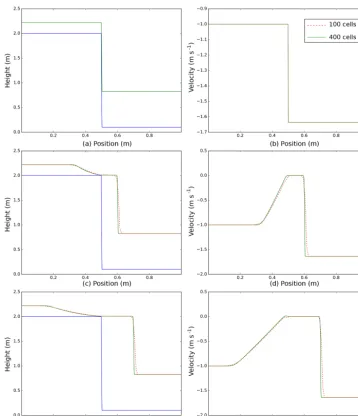
Figure 2.1-D Riemann problem with no friction. Numerical solution at three different times: 0 s(a, b), 0.1 s(c, d), 0.2 s(e, f). Flow thickness and bottom topography (blue line) are plotted in the left panels, while the velocity is plotted in the right panels. The different colors represent numerical solutions obtained with different numbers of cells: 100 (dashed red line) and 400 (solid green line).
a left-going rarefaction wave and a right-going shock wave. We present here the numerical solution obtained with a three-step IMEX Runge–Kutta scheme, whereby the reconstruc-tion from the cell centers to the faces is applied to the phys-ical variables. The solutions obtained by discretizing the do-main with 100 cells (Fig. 2, dashed red lines) and 400 cells (Fig. 2, solid green lines) are compared. The numerical re-sults at two different timest >0 (Fig. 2, middle and bottom panels) show the capacity of the numerical scheme to prop-erly model the propagation of both the rarefaction and shock waves, and the good description of the shock with a small number of cells highlights the low numerical diffusivity of the central-upwind finite-volume numerical scheme imple-mented for the spatial discretization of the governing equa-tions.
4.2 One-dimensional problem with dry–wet interface and friction
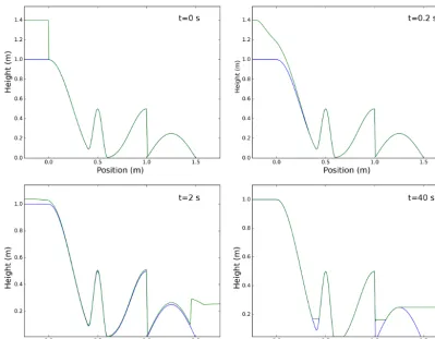
Figure 3.Numerical solution of a 1-D Riemann problem with friction at four different times. The solid blue line represents the topography, while the solid green line represents the free surface of the wet region.
as follows:
B(x)=
1, x≤0,
cos2(π x), 0≤x <0.4, cos2(π x)+0.25(cos(10π(x−0.5))+1), 0.4≤x <0.5, 0.5cos4(π x)+0.25(cos(10π(x−0.5))+1), 0.5≤x <0.6, 0.5cos4(π x), 0.6≤x <1, 0.25 sin(2π(x−1)), 1≤x <1.5,
0, x≥1.5.
The initial conditions are defined by w(x,0)=
1.4, x≤0,
B(x), x >0, u(x,0)=0.
For this simulation, the gravitational constant has a value g=1 and a simpler friction term is employed (−κ(h)u, with κ(h)=0.001(1+10h)−1). Also, for this test the numerical solution is obtained with a three-step IMEX Runge–Kutta scheme, whereby the reconstruction from the cell centers to the faces has been applied to the physical variables and the domain [−0.25;1.75] has been discretized with 400 cells. The boundary conditions are prescribed to model a closed domain and also to check that the total mass contained in the domain is kept constant by the numerical discretiza-tion schemes. The numerical soludiscretiza-tion at four different times
(t=0, t=0.2, t=2 and t=40 s) is presented in Fig. 3, showing the capability of the model to deal with the prop-agation of dry–wet interfaces and to reach a steady solution for which the horizontal gradient ofw=h+Bis null. 4.3 One-dimensional pyroclastic avalanche with
Voellmy–Salm friction
This example is a 1-D test for the Voellmy–Salm rheology, with a pile of material initially at rest released on a con-stant slope topography. This test is aimed at checking if the model is able to preserve an initial steady condition, when the tangent of the pile free surface slope is smaller than the Coulomb friction coefficient, µ, and to properly simulate the stopping of the flow, i.e., when inertial and gravitational forces are smaller than total basal friction.
For this test, the domain is the interval[0;500] and the center of the pile coincides with the center of the domain. The gravitational constant isg=9.81 ms−2and the parameters of the Voellmy–Salm rheology areµ=0.3 andξ =300 ms−2.
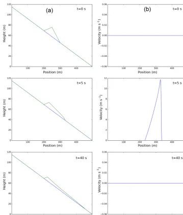
Figure 4.Numerical solution of a 1-D problem with Voellmy–Salm friction at three different times. In(a)the topography (blue line) and the profile of the material (green line) are plotted. In(b)the corresponding velocities are shown.
steady and the pile of material starts to move along the slope until it reaches the stoppage condition.
The numerical solution at three different times (t=0, t=5 andt=40 s) is presented in Fig. 4. For this simulation, the reconstruction technique with limiters has been applied to the physical variables and an IMEX four-step Runge–Kutta has been adopted, while the domain has been discretized with 400 cells. The plot of the numerical solution at the interme-diate time clearly shows that the front of the flow has a larger propagation velocity than the rest of the flow. On the other hand, comparing the left and right middle panels, we ob-serve that part of the tail is not moving at all. After a few tens of seconds from the release, the flow reaches a steady condition, as shown by the plot of the velocity at 40 s (bot-tom right panel in Fig. 4). This test highlights the capability
of the model to reach a steady condition not only when the gradient ofw=h+Bis null, as shown in the previous exam-ple, but also with a flow with a positive slope below a critical condition.
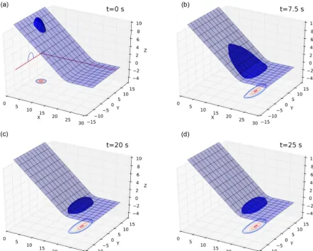
4.4 Two-dimensional pyroclastic avalanche with Voellmy–Salm friction
Figure 5.Numerical simulation of two-dimensional pyroclastic avalanche with Voellmy–Salm friction. The contour plots on the bottom plane of each panel represent constant values of the thickness of the flow, whose free surface is represented in blue. The outermost contour on the bottom plane corresponds to a thickness of 0.06 m, and thus the thinner portion of the flow is not represented by the contour plot. A visual comparison between the two bottom plots highlights the fact that a steady condition has been reached.
the rectangle[0;30]×[−7;7], in which a hemispherical shell holding the material together with a maximum thickness of 1.85 m is suddenly released so that the bulk material starts to slide on an inclined flat plane at 35◦ (for 0≤x≤17.5) into a horizontal run-out plane (forx≥21.5) connected by a smooth transition. Here we do not use the same rheological model as in the original paper of the example, but a Voellmy– Salm rheology is applied withµ=0.3 andξ =300 ms−2.
The numerical solution at four different times (t=0,t= 7.5,t=20 andt=25 s) is presented in Fig. 5, in which both the three-dimensional flow shape over the topography and thickness contours are presented. For this simulation, the re-construction technique with limiters has been applied to the physical variables and an IMEX two-step Runge–Kutta has been adopted, while the domain has been discretized with 150×100 cells.
As shown by the plots presented in Fig. 5, the model is able to simulate the propagation of the flow with no
numer-ical oscillations or instabilities, without the need for artifi-cial numerical diffusion. As the front reaches the maximum run-out and horizontal spreading (top left panel), the tail of the flow is still accelerating and the avalanche body starts to contract. Comparing the two panels at the bottom, it is evi-dent that after about 20 s the flow has stopped propagating, with the deposit located at the transition region between the inclined and horizontal zones. This simulation took 238 s on an Intel Core i5-3210M CPU at 2.50 GHz.
5 Simulation of a pyroclastic avalanche at Etna volcano
Vul-Figure 6.Map of the avalanche deposit from the February 2014 pyroclastic avalanche and the lava flow.
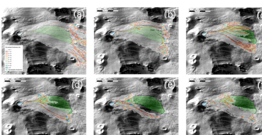
Figure 7.Results of IMEX_SfloW2D numerical simulations of a pyroclastic avalanche overlapped on the hill-shaded relief of the Etna summit and the boundaries of the 11 February 2014 event. Numerical parameters as follows:(a)µ=0.1,ξ=500;(b)µ=0.2,ξ=500;
(c)µ=0.2,ξ=100;(d)µ=0.3,ξ=500;(e)µ=0.4,ξ=500;(f)µ=0.4,ξ=5000. Avalanche volume is equal to 0.5×10⁶m3.
canologia) monitoring system and, in particular, it was filmed by the thermal IR camera from Monte Cagliato, located on the east slope of the Valle del Bove at about 7 km from the NSEC, and the Catania CUAD visible camera (ECV) about 26 km south of the summit. A 500 m wide avalanche front propagated about 2.3 km along the steep slopes of the Valle del Bove before stopping at the break in slope at the val-ley bottom. At the same time, a voluminous buoyant ash
activity, it was unfortunately not possible to obtain a detailed map of the deposit thickness. Comparison of numerical re-sults will therefore be limited to the flow boundary and run-out.
IMEX_SfloW2D numerical simulations have been per-formed over the 2014 digital elevation model of Mount Etna (De Beni et al., 2015). We have developed a MATLAB tool to modify the original topography by excavating a detaching volume with an ellipsoidal shape oriented towards the local maximum slope and with a prescribed total volume. The ini-tial avalanche volume is defined by the difference between the original and the modified topography. It is also worth re-marking that the DEM did not account for the presence of the thick lava flow that had been emplaced in the days be-fore the avalanche event (Fig. 6), which likely controlled the avalanche path by confining it along its southern edge (An-dronico et al., 2018).
The avalanche rheological parameters have been varied in ranges consistent with previous studies of geophysical gran-ular avalanches (e.g., Bartelt et al., 1999). For quasi-static granular flows,µis physically related to the basal friction of the granular material. However, its value for rapid avalanches cannot be easily defined a priori. We thus simply considerµ andξas empirical model parameters whose values need to be calibrated. In particular, 0.2< µ <0.5 and 300< ξ <5000. Results of computations are reported graphically in Fig. 7.
The misfit between the simulated and observed flow path is due to the presence of the lava flow depicted in Fig. 6 that was not included in the DEM. Overall, the fit is reasonable in terms of maximum run-out and area covered by the modeled deposit for runs (d)(µ=0.3, ξ=500)and (f)(µ=0.4, ξ= 5000). It is interesting to note that the value µ=0.3−0.4 corresponds to fairly low friction coefficients of dry granular materials (corresponding to repose angles of 16–20◦). This observation is commonly acknowledged as frictional weak-ening for rapid granular flows (e.g., Lucas et al., 2014).
A thorough discussion about the optimal choice of the rheological model and parameters for pyroclastic avalanches would require an extensive comparison with similar phenom-ena that occurred at Etna (few of which have been docu-mented so far) and at other analogous volcanoes, for which more accurate measurements will be needed in the future to achieve a better calibration of the model. This, is however, clearly beyond the scope of the present work.
6 Conclusions
We have presented the physical formulation, numeri-cal solution strategy and verification tests of the new IMEX_SfloW2D numerical model for shallow granular avalanches. The numerical code is available open-source and freely downloadable from a GIT repository, where the users can also find the documentation and example tests described in this paper. The main features of the new model make it
suited for research and application to geophysical granular avalanches, in particular the following.
– The flexible discretization and numerical solution algo-rithm (not tied to knowledge of the eigenstructure of the system of equations) allows for the easy implementation of new transport equations.
– The formulation in Cartesian geographical coordinates is suited for running on digital surface models (read in standard ESRI ASCII grid format) and for the integra-tion of non-hydrostatic terms, even on steep slopes. – The conservative and positivity-preserving numerical
scheme allows for a robust and accurate tracking of 1-D and 2-1-D discontinuities, including wet–dry interfaces and flow fronts.
– The implicit coupling of nonlinear rheology terms al-lows for the simulation of steady-state equilibrium so-lutions and, in particular, favors flow stopping without the need for any ad hoc empirical criteria.
– The numerical procedure to evaluate the Jacobian of the nonlinear system (based on a complex-step derivative technique) allows for an easy implementation and test-ing of new rheological models for complex geophysical granular avalanches.
Code availability. The numerical code, benchmark tests and doc-umentation are available at https://github.com/demichie/IMEX_ SfloW2D (last access: 30 January 2019). Preprocessing scripts (to change the grid resolution and the numerical schemes) and post-processing scripts (to plot the solution variables and to create anima-tions) are also available. Furthermore, each example has a page de-scription on the model Wiki (https://github.com/demichie/IMEX_ SfloW2D/wiki, last access: 30 January 2019), where detailed infor-mation on how to run the simulations is given. The digital object identifier (DOI) for the version of the code documented in this pa-per is https://doi.org/10.5281/zenodo.2553101 (de’ Michieli Vitturi and Lari, 2019).
Author contributions. MdMV has developed the numerical algo-rithm and implemented the 1-D model and numerical tests. TEO has contributed to the model formulation and application in the context of volcanological applications. GL has implemented the numerical scheme and algorithm in 2-D. AA has tested the model and helped with the comparison to similar depth-averaged models in volcanol-ogy.
Competing interests. The authors declare that they have no conflict of interest.
task D1. We warmly thank Daniele Andronico, Emanuela De Beni and Boris Behncke for useful discussions about the Etna 2014 event and for providing field data and the digital elevation model. TEO would like to thank Perry Bartelt and Betty Sovilla (SLF, Switzerland) for stimulating discussions on granular avalanches and density currents. The authors are also grateful to Olivier Roche and Karim Kelfoun for their careful review and useful and constructive comments. Mattia de’ Michieli Vitturi and Giacomo Lari gratefully acknowledge Andrea Milani, whose contribution to the career and numerical work of the two authors was of great significance.
Edited by: Simone Marras
Reviewed by: Karim Kelfoun and Olivier Roche
References
Andrianov, N.: Testing numerical schemes for the shallow wa-ter equations, Tech. rep., available at: https://github.com/ nikolai-andrianov/CONSTRUCT/blob/master/testing_sw.pdf (last access: 30 January 2019), 2004.
Andronico, D., Di Roberto, A., De Beni, E., Behncke, B., Antonella, B., Del Carlo, P., and Pompilio, M.: Pyroclas-tic density currents at Etna volcano, Italy: The 11 Febru-ary 2014 case study, J. Volcanol. Geoth. Res., 357, 92–105, https://doi.org/10.1016/j.jvolgeores.2018.04.012, 2018. Ascher, U. M., Ruuth, S. J., and Spiteri, R. J.: Implicit-explicit
Runge-Kutta methods for time-dependent partial differential equations, Appl. Numer. Math., 25, 151–167, 1997.
Bartelt, P., Salm, L. B., and Gruberl, U.: Calculating dense-snow avalanche runout using a Voellmyfluid model with ac-tive/passive longitudinal straining, J. Glaciol., 45, 242–254, https://doi.org/10.3189/002214399793377301, 1999.
Bartelt, P., Buser, O., Valero, C. V., and Bühler, Y.: Configu-rational energy and the formation of mixed flowing/powder snow and ice avalanches, Ann. Glaciol., 57, 179–188, https://doi.org/10.3189/2016aog71a464, 2016.
Benjamin, T. B.: Gravity currents and related phenomena, J. Fluid Mech., 31, 209–248, 1968.
Bursik, M. I. and Woods, A. W.: The dynamics and ther-modynamics of large ash flows, B. Volcanol., 58, 175–193, https://doi.org/10.1007/s004450050134, 1996.
Castro-Orgaz, O., Hutter, K., Giraldez, J. V., and Hager, W. H.: Nonhydrostatic granular flow over 3-D terrain: New Boussinesq-type gravity waves?, J. Geopys. Res., 120, 1–28, https://doi.org/10.1002/2014jf003279, 2015.
Charbonnier, S. J. and Gertisser, R.: Numerical simulations of block-and-ash flows using the Titan2D flow model: examples from the 2006 eruption of Merapi Volcano, Java, Indonesia, B. Volcanol., 71, 953–959, https://doi.org/10.1007/s00445-009-0299-1, 2009.
Christen, M., Kowalski, J., and Bartelt, P.: RAMMS: Numerical simulation of dense snow avalanches in three-dimensional ter-rain, Cold Reg. Sci. Technol., 63, 1–14, 2010.
Dade, W. B.: The emplacement of low-aspect ratio ignimbrites by turbulent parent flows, J. Geophys. Res., 108, 1–9, https://doi.org/10.1029/2001JB001010, 2003.
Dade, W. B. and Huppert, H. E.: Emplacement of the Taupo ign-imbrite by a dilute turbulent flow, Nature, 381, 509–512, 1996. De Beni, E., Behncke, B., Branca, S., Nicolosi, I., Carluccio, R.,
D’Ajello Caracciolo, F., and Chiappini, M.: The continuing story of Etna’s New Southeast Crater (2012–2014): Evolution and vol-ume calculations based on field surveys and aerophotogramme-try, J. Volcanol. Geoth. Res., 303, 175–186, 2015.
Delannay, R., Valance, A., Mangeney, A., Roche, O., and Richard, P.: Granular and particle-laden flows: from labora-tory experiments to field observations, J. Phys. D, 50, 1–40, https://doi.org/10.1088/1361-6463/50/5/053001, 2017.
de’ Michieli Vitturi, M. and Lari, G.: IMEX_SfloW2D v. 1.0.0 (Ver-sion 1.0.0), Zenodo, https://doi.org/10.5281/zenodo.2553101, 2019.
Denlinger, R. P. and Iverson, R. M.: Flow of variably fluidized gran-ular masses across three-dimensional terrain: 2. Numerical pre-dictions and experimental tests, J. Geophys. Res., 106, 553–566, https://doi.org/10.1029/2000jb900330, 2001.
Denlinger, R. P. and Iverson, R. M.: Granular avalanches across irregular three-dimensional terrain: 1. The-ory and computation, J. Geophys. Res., 109, F01014, https://doi.org/10.1029/2003JF000085, 2004.
Doyle, E. E., Hogg, A. J., Mader, H. M., and Sparks, R. S. J.: A two-layer model for the evolution and propagation of dense and dilute regions of pyroclastic currents, J. Volcanol. Geoth. Res., 190, 365–378, https://doi.org/10.1016/j.jvolgeores.2009.12.004, 2010.
Dufek, J.: The Fluid Mechanics of Pyroclastic Den-sity Currents, Annu. Rev. Fluid Mech., 48, 459–485, https://doi.org/10.1146/annurev-fluid-122414-034252, 2015. Engwell, S., de’ Michieli Vitturi, M., Esposti Ongaro, T., and Neri,
A.: Insights into the formation and dynamics of coignimbrite plumes from one-dimensional models, J. Geophys. Res.-Sol. Ea., 121, 4211–4231, 2016.
Esposti Ongaro, T., Orsucci, S., and Cornolti, F.: A fast, calibrated model for pyroclastic density currents kinemat-ics and hazard, J. Volcanol. Geoth. Res., 327, 257–272, https://doi.org/10.1016/j.jvolgeores.2016.08.002, 2016. Fischer, J.-T., Kowalski, J., and Pudasaini, S. P.:
To-pographic curvature effects in applied avalanche modeling, Cold Reg. Sci. Technol., 74–75, 21–30, https://doi.org/10.1016/j.coldregions.2012.01.005, 2012. Fisher, R. V.: Decoupling of pyroclastic currents:
haz-ards assessments, J. Volcanol. Geoth. Res., 66, 257–263, https://doi.org/10.1016/0377-0273(94)00075-r, 1995.
Fisher, R. V., Orsi, G., Ort, M., and Heiken, G.: Mobility of a large-volume pyroclastic flow–emplacement of the Campa-nian ignimbrite, Italy, J. Volcanol. Geoth. Res., 56, 205–220, https://doi.org/10.1016/0377-0273(93)90017-l, 1993.
Forterre, Y. and Pouliquen, O.: Flows of Dense Gran-ular Media, Annu. Rev. Fluid Mech., 40, 1–24, https://doi.org/10.1146/annurev.fluid.40.111406.102142, 2008. Guo, Y. and Curtis, J. S.: Discrete Element Method Simulations for
Complex Granular Flows, Annu. Rev. Fluid Mech., 47, 21–46, https://doi.org/10.1146/annurev-fluid-010814-014644, 2015. Iverson, R. M. and Denlinger, R. P.: Flow of variably fluidized
Iverson, R. M. and George, D. L.: A depth-averaged debris-flow model that includes the effects of evolving dila-tancy. I. Physical basis, P. R. Soc. A, 470, 20130819, https://doi.org/10.1098/rspa.2013.0819, 2014.
Kelfoun, K.: Suitability of simple rheological laws for the numerical simulation of dense pyroclastic flows and long-runout volcanic avalanches, J. Geophys. Res., 116, B08209, https://doi.org/10.1029/2010JB007622, 2011.
Kelfoun, K.: A two-layer depth-averaged model for both the dilute and the concentrated parts of pyroclastic currents, J. Geophys. Res.-Sol. Ea., 122, 4293–4311, https://doi.org/10.1002/2017JB014013, 2017a.
Kelfoun, K.: A two-layer depth-averaged model for both the dilute and the concentrated parts of pyroclastic currents, J. Geophys. Res.-Sol. Ea., 122, 4293–4311, 2017b.
Kelfoun, K. and Druitt, T. H.: Numerical modeling of the emplace-ment of Socompa rock avalanche, Chile, J. Geophys. Res.-Sol. Ea., 110, B12202, https://doi.org/10.1029/2005JB003758, 2005. Komorowski, J.-C., Jenkins, S., Baxter, P. J., Picquout, A., Lav-igne, F., Charbonnier, S., Gertisser, R., Preece, K., Cho-lik, N., Budi-Santoso, A., and Surono: Paroxysmal dome explosion during the Merapi 2010 eruption: Processes and facies relationships of associated high-energy pyroclastic density currents, J. Volcanol. Geoth. Res., 261, 260–294, https://doi.org/10.1016/j.jvolgeores.2013.01.007, 2013. Kurganov, A. and Petrova, G.: A second-order well-balanced
pos-itivity preserving central-upwind scheme for the Saint-Venant system, Commun. Math. Sci., 5, 133–160, 2007.
La Spina, G. and de’ Michieli Vitturi, M.: High-resolution finite vol-ume central schemes for a compressible two-phase model, SIAM J. Sci. Comput., 34, B861–B880, 2012.
Lucas, A., Mangeney, A., and Ampuero, J. P.: Frictional velocity-weakening in landslides on Earth and on other planetary bodies, Nat. Commun., 5, 1–9, https://doi.org/10.1038/ncomms4417, 2014.
Mangeney, A., Bouchut, F., Thomas, N., Vilotte, J. P., and Bris-teau, M. O.: Numerical modeling of self-channeling granular flows and of their levee-channel deposits, J. Geophys. Res., 112, F02017, https://doi.org/10.1029/2006JF000469, 2007.
Mangeney-Castelnau, A., Vilotte, J.-P., Bristeau, M.-O., Perthame, B., Bouchut, F., Simeoni, C., and Yerneni, S.: Numerical modeling of avalanches based on Saint Venant equations us-ing a kinetic scheme, J. Geophys. Res.-Sol. Ea., 108, 2527, https://doi.org/10.1029/2002JB002024, 2003.
Martins, J. R. R. A., Sturdza, P., and Alonso, J. J.: The complex-step derivative approximation, ACM T. Math. Software, 29, 245–262, https://doi.org/10.1145/838250.838251, 2003.
Oberkampf, W. L. and Trucano, T. G.: Verification and validation in computational fluid dynamics, Prog. Aerosp. Sci., 38, 209–272, 2002.
Ogburn, S. E. and Calder, E. S.: The Relative Effective-ness of Empirical and Physical Models for Simulating the Dense Undercurrent of Pyroclastic Flows under Differ-ent EmplacemDiffer-ent Conditions, Front. Earth Sci., 5, 63–26, https://doi.org/10.3389/feart.2017.00083, 2017.
Pareschi, L. and Russo, G.: Implicit–explicit Runge–Kutta schemes and applications to hyperbolic systems with relaxation, J. Sci. Comput., 25, 129–155, 2005.
Patra, A. K., Bauer, A., Nichita, C., Pitman, E. B., Sheridan, M., Bursik, M., Rupp, B., Webber, A., Stinton, A., Namikawa, L., and Renschler, C. S.: Parallel adaptive numerical simulation of dry avalanches over natural terrain, J. Volcanol. Geoth. Res., 139, 1–21, 2005.
Pitman, E. B., Nichita, C. C., Patra, A., Bauer, A., Sheridan, M., and Bursik, M.: Computing granular avalanches and landslides, Phys. Fluids, 15, 3638–3646, https://doi.org/10.1063/1.1614253, 2003.
Press, W. H., Teukolsky, S. A., Vetterling, W. T., and Flannery, B. P.: Numerical recipes in Fortran 90, vol. 2, Cambridge university press Cambridge, 1996.
Pudasaini, S. P. and Hutter, K.: Avalanche dynamics: dynamics of rapid flows of dense granular avalanches, Springer Science & Business Media, 2007.
Shea, T., Gurioli, L., Houghton, B. F., Cioni, R., and Cash-man, K. V.: Column collapse and generation of pyroclas-tic density currents during the A.D. 79 eruption of Vesu-vius: The role of pyroclast density, Geology, 39, 695–698, https://doi.org/10.1130/g32092.1, 2011.
Shimizu, H. A., Koyaguchi, T., and Suzuki, Y. J.: A numerical shallow-water model for gravity currents for a wide range of density differences, Progress in Earth and Planetary Science, 4, 1–13, https://doi.org/10.1186/s40645-017-0120-2, 2017. Simpson, J. E.: Gravity currents: In the environment and the
labo-ratory, Cambridge University Press, 1999.
Toro, E. F.: Riemann solvers and numerical methods for fluid dy-namics: a practical introduction, Springer Science & Business Media, 2013.
Von Karman, T.: The engineer grapples with nonlinear problems, B. Am. Math. Soc., 46, 615–683, 1940.
Wang, Y., Hutter, K., and Pudasaini, S. P.: The Savage-Hutter the-ory: A system of partial differential equations for avalanche flows of snow, debris, and mud, ZAMM-Z. Angew. Math. Me., 84, 507–527, 2004.
Woods, A. W. and Wohletz, K.: Dimensions and dynamics of co-ignimbrite eruption columns, Nature, 350, 225–227, https://doi.org/10.1038/350225a0, 1991.
Woods, A. W., Bursik, M. I., and Kurbatov, A. V.: The interaction of ash flows with ridges, B. Volcanol., 60, 38–51, 1998. Yuan, L., Liu, W., Zhai, J., Wu, S. F., Patra, A. K., and Pitman, E. B.: