www.geosci-instrum-method-data-syst.net/6/193/2017/ doi:10.5194/gi-6-193-2017
© Author(s) 2017. CC Attribution 3.0 License.
Application of particle swarm optimization for gravity inversion of
2.5-D sedimentary basins using variable density contrast
Kunal Kishore Singh1,2and Upendra Kumar Singh1
1Department of Applied Geophysics, IIT(ISM), Dhanbad 826004, India 2Geological Survey of India, Lucknow-226024, India
Correspondence to:Upendra Kumar ([email protected]) Received: 23 March 2016 – Discussion started: 25 August 2016
Revised: 1 March 2017 – Accepted: 11 March 2017 – Published: 10 April 2017
Abstract.Particle swarm optimization (PSO) is a global op-timization technique that works similarly to swarms of birds searching for food. A MATLAB code in the PSO algorithm has been developed to estimate the depth to the bottom of a 2.5-D sedimentary basin and coefficients of regional back-ground from observed gravity anomalies. The density con-trast within the source is assumed to vary parabolically with depth. Initially, the PSO algorithm is applied on synthetic data with and without some Gaussian noise, and its validity is tested by calculating the depth of the Gediz Graben, west-ern Anatolia, and the Godavari sub-basin, India. The Gediz Graben consists of Neogen sediments, and the metamorphic complex forms the basement of the graben. A thick unin-terrupted sequence of Permian–Triassic and partly Jurassic and Cretaceous sediments forms the Godavari sub-basin. The PSO results are better correlated with results obtained by the Marquardt method and borehole information.
1 Introduction
The gravity method is a natural source method which helps in locating masses of greater or lesser density than the sur-rounding formations. It is used as a reconnaissance survey in hydrocarbon exploration. Sedimentary basins, which are characterized by negative gravity anomalies, are the loca-tion of almost all of the world’s hydrocarbon reserves. In-terpretation of gravity data is a mathematical process of try-ing to optimize the parameters of the initial model in or-der to get a good match to the observed data. Interpreta-tion of gravity data is always associated with the ambigu-ity problem. Ambiguambigu-ity in gravambigu-ity anomalies can be
over-come by assigning a mathematical geometry to the anomaly-causing body with a known density contrast (Rama Rao and Murthy, 1978). Bott (1960) used stacked prism model to de-scribe the cross-section of a sedimentary basin, whereas Tal-wani (1959) used the polygonal model to describe source ge-ometry. The parabolic density function is used to remove the complications associated with exponential (Cordell, 1973), cubic (Garcia-Abdeslem, 2005) and quadratic (Gallardo-Delgado et al., 2003) density functions. The Marquardt inver-sion through residual gravity anomalies delineates the struc-ture of a sedimentary basin by estimating regional back-ground (Chakravarthi and Sundararajan, 2007; Marquardt, 1963). Several authors have developed 2-D/2.5-D local op-timization techniques over the 2-D/2.5-D sedimentary basin (Annecchione et al., 2001; Barbosa et al., 1999; Bhattacharya and Navolio, 1975; Gadirov et. al, 2016; Litinsky, 1989; Mor-gan and Grant, 1963; Murthy et al., 1988; Murthyan and Rao, 1989; Rao, 1994; Won and Bavis, 1987) to interpret gravity anomalies with constant density function. In many publica-tions over 3-D gravity field computation with an approxima-tion of geological bodies by 3-D polygonal horizontal prism has been applied (Eppelbaum and Khesin, 2004; Khesin et al. 1996). Rao (1990) used a quadratic density function, which is comparatively reliable, to analyse gravity anomalies over basins having a limited thickness, whereas Chakravarthi and Rao (1993) carried out modelling and inversion of gravity anomalies with a parabolic density function.
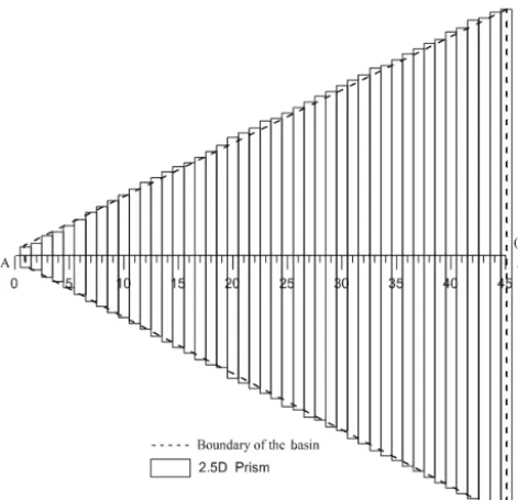
Figure 1.The 2.5-D sedimentary basin and its approximation by juxtaposing prisms.
MATLAB code based on PSO is developed to interpret the gravity anomalies of 2.5-D sedimentary basins, where the density varies parabolically with depth. PSO-analysed results are consistent with and more accurate than other techniques and also agree significantly well with borehole information.
2 Theory
In Bott’s approach, a sedimentary basin is approximated by a series of vertical prisms. The gravity anomalygbat any point on the profileAA0as shown in Fig. 1.
gb= N−1
X
j=2
gj(xl,0)+Cx+D (1)
The gravity effect oflth prism is given as
g(xl,0)= z2 Z z=z1 a Z y=−a c Z x=−c
G1ρ(z)zdxdydz
(x−x1)2+y2+z23/2
. (2)
The parabolic density function at any depthwis given by
1ρ(w)= 1ρ
3 0
(1ρ0−αw)2
. (3)
Finally, after integration of Chakravarthi and Sundarara-jan (2006), Eq. (2) becomes
g(xl,0)= −2G1ρ03 (4)
* αx1L p4 1 p2 + 1 p3
lnp5 p6
+ L 2p2
ln(K+x1) (K−x1)
+ x1 2p3
ln(K+L) (K−L)+ 1ρ0
α
1 p2
tan−1
KL zx1 + 1 p3 tan−1
x1L
zL
− 1 αp5
tan−1
Lx1
zL
+
x1+c
x1−c
z2 z1 , where
K= x12+L2+z2,
p1=x12+L2, p2=L2α2+1ρ02,
p3=x12+1ρ02, p4=
q
p1α2+1ρ02,
p5=1ρ02−αz,
p6= −2 αKp4+p1α2+1ρ0αz.
Here,N is the number of observations, Gis the universal gravitational constant,C andDare coefficients of regional background,cis half width of the prism,z1andz2are depths to the top and bottom of the basin, 2Lis strike length of the prism, a is the offset of the profile from the centre of the prism and1ρ0andαare constants of the parabolic density function at depthz.
Since the profileAA0does not pass through the centres of each prism, Eq. (4) has to be calculated twice by puttingL−a
andL+aforLand taking the average. The initial depths of the basin calculated using observed anomalyg0are given as
di=
g0(xi)1ρ
41.891ρ02+αg0(xi)
, i=2,3,4, . . .N−1. (5)
The profileAA0entirely covers the lateral dimensions of the sedimentary basin; therefore the depth of the basin on either side of the profile become zero. So,d1=0=dN
2.1 Particle swarm optimization
and Das, 2013).
Vtk=wVtk−1+c1·rand1·
Pbestt−Xtk
+c2·rand2·
Gbest−Xkt, (6)
Xtk=Xk−t 1+Vtk, (7)
wherekis the number of iterations;tis the particle number;
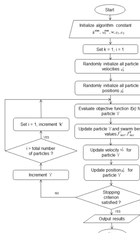
Vtk is the velocity of thetth particle atkiterations;Xtkis the position oftth particle atkiterations;Pbestt is the best po-sition of individualtth particle (local best position);Gbest is the best position of all particles (global best position); rand1 and rand2are the independent uniformly random numbers in the range [0, 1]; c1 andc2 are the positive learning factor which controls the maximum step length; and w is the in-ertial weight factor that controls the speed of the particles. Equation (7) gives the updated velocity based on the current velocity, current position, local, best position and global best position. This process is repeated until the desired result is obtained. The schematic diagram/flow chart of the PSO al-gorithm is shown in Fig. 2.
2.2 Examples
The MATLAB code based on PSO is applied to a synthetic model of a sedimentary basin and real field data sets from Gediz Graben, western Anatolia, and the Godavari sub-basin, India.
2.3 Synthetic Example
We have used a synthetic gravity anomaly of 45×103m length at a 1.0×10³m station interval. In Bott’s algorithm, the prism will be of equal width, 1.0×10³m, but with different strike lengths. Here parabolic density function is used with the constants1ρ0= −0.65×10³Kg m−3andα= 0.04×10³Kg m−3per 1000 m. The profile does not bisect the strike lengths of prism, and so offset distance of the profile from the centre of each prism is mentioned in the code. We have added an interference term, Ax+B, with
A= −0.007 mgal per 1000 m andB= −10 mgal for the re-gional background. The required result is found at 15 itera-tions with a root mean square error (RMSR) of 2.9369e−006 from the Marquardt algorithm.
We have used the same synthetic gravity anomaly for the PSO algorithm. The Fig. 3 shows the learning process of
Pbest andGbest in terms of error and iterations. The best result is found with 57 iterations and 50 models (Fig. 3). So it is seen that after 57 iterations and 50 models, the calcu-lated anomalies match the synthetic anomaly and estimated depths coincide with the actual structure where the RMSE is 2.8383e−004. Gaussian noises of 5 and 10 % are added to the synthetic data to perceive the robustness of the PSO algorithm. PSO does not find the true depths, but it gives val-ues close to the true depths. The upper part of Fig. 4 shows
Figure 2.The detail schematic diagram/flow chart of PSO tech-niques.
the synthetic and PSO-calculated gravity anomalies of a syn-thetic model of a 2.5-D sedimentary basin, and the lower part shows the inferred depth structure obtained from the PSO and Marquardt algorithm for synthetic data. Figures 5 and 6 show the synthetic data with 5 and 10 % Gaussian noises and cal-culated gravity anomalies obtained from the PSO algorithm, and inferred depth structure obtained by the PSO and Mar-quardt algorithm.
3 Field example
3.1 Gediz Graben, western Anatolia
dif-Figure 3.Iteration verses RMSE ofPbest andGbest using the PSO technique through synthetic gravity anomaly.
Figure 4.Synthetic and calculated gravity anomalies with parabolic density function due to a synthetic model of a 2.5-D sedimentary basin, obtained from the PSO algorithm, and inferred depth struc-ture obtained from the PSO and Marquardt algorithm.
ferent strike lengths, whereas Chakravarthi and Sundarara-jan (2007) used the same prism and interpreted gravity anomaly by the Marquardt algorithm using a parabolic den-sity function whose constants are1ρ0= −1.407×10³and
α=2.26935×10³Kg m−3per 1000 m.
We have used a similar number of prisms in PSO to im-prove the results. So with 65 iterations and 50 models, we achieve a good fit between observed and PSO-analysed grav-ity anomalies with a RMSE of 0.0083. The maximum thick-ness of the graben is inferred as 1.87×10³m, which matches well with 1.8×10³m as estimated by Sari and Salk (2002), as compared to 1.64×10³m obtained by Chakravarthi and Sun-dararajan (2007). The upper part of Fig. 7 shows the observed and PSO-calculated gravity anomalies over Gediz Graben, western Anatolia, and the lower part show the inferred depth structure obtained from the PSO and Marquardt algorithm. 3.2 Godavari sub-basin
The Godavari sub-basin is one of the major basins of the Pranhita–Godavari valleys (Rao, 1982), whose approximate strike length is 220×103m. The gravity profile is taken for
Figure 5.Synthetic data with 5 % Gaussian noise and calculated gravity anomalies obtained from the PSO algorithm, and inferred depth structure obtained from the PSO and Marquardt algorithm.
Figure 6.Synthetic data with 10 % Gaussian noise and calculated gravity anomalies obtained from the PSO algorithm, and inferred depth structure obtained from the PSO and Marquardt algorithm.
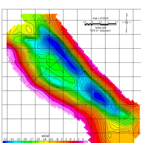
study from the residual Bouguer gravity anomaly map of the Godavari sub-basin as shown in Fig. 8. We have used 29 vertical prisms, each with equal widths of 2.0×10³m but with different strike lengths for sedimentary basin modelling. The constants of parabolic density functions used for the Go-davari sub-basin are1ρ0= −0.5×10³andα=0.1518259× 10³Kg m−3 per 1000 m (Chakravarthi and Sundararajan, 2004). So with 71 iterations and 45 models, we achieve a good fit between observed and PSO-analysed gravity anoma-lies. The RMSE is 0.0099. The maximum depth of the basin, obtained from PSO, is 4.09×10³m, which is quite close to the borehole information (Agarwal, 1995). Chakravarthi and Sundararajan (2005) obtained a maximum depth of 4.0×
up-Figure 7.Observed and calculated gravity anomalies with parabolic density function, Gediz Graben, western Anatolia, obtained from the PSO algorithm, and inferred structure obtained from the PSO and Marquardt algorithm.
Figure 8.Residual Bouguer gravity anomaly map of the Godavari sub-basin (modified after Chakravarthi and Sundararajan, 2005) and gravity anomaly profile taken for study.
per part of Fig. 9 shows the variation of observed and PSO-calculated gravity anomalies of the Godavari sub-basin, and the lower part shows the inferred structure obtained from the PSO and Marquardt algorithm.
Figure 9.Observed and calculated residual Bouguer gravity anoma-lies of parabolic density function of the Godavari sub-basin ob-tained from the PSO algorithm, and inferred depth structure from the PSO and Marquardt algorithm.
4 Conclusions
Particle swarm optimization in the MATLAB environment has been developed to estimate the model parameters of a 2.5-D sedimentary basin where the density contrast varies parabolically with depth. We have implemented the PSO al-gorithm on synthetic data with and without Gaussian noise and two field data sets. An observation has made that PSO is affected by some levels of noise, but estimated depths are close to the true depths. The results obtained from PSO us-ing synthetic and field gravity anomalies are well correlated with borehole samples and provide more geological viabil-ity. Despite its long computation time, PSO is very simple to implement and is controlled by only one operator.
Data availability. Our paper presents the applicability and poten-tiality of PSO in gravity inverse problems. First, PSO is validated on synthetic gravity anomalies with and without noise, and the de-veloped PSO-based algorithm is finally applied over two kinds of field gravity data taken from different geological terrains: (i) resid-ual gravity anomaly over Gradiz Graben, western Anatolia (Sari and Salk, 2002), and (ii) residual gravity anomaly taken from Godavari sub-basin, India (Chakravarthi and Sundararajan, 2004).
Competing interests. The authors declare that they have no conflict of interest.
the financial support to develop the infrastructre.
Edited by: L. Eppelbaum
Reviewed by: Gadirov and one anonymous referee
References
Agarwal, B. P.: Hydrocarbon prospects of the Pranhita-Godavari Graben, India, Proceedings of Petrotech 95, 115–121, 1995. Annecchione, M. A., Chouteau, M., and Keating, P.:Gravity
inter-pretation of bedrock topography: the case of the Oak Ridges Moraine, Southern Ontario, Canada, J. Appl. Geophys., 47, 63– 81, 2001.
Barbosa, V. C. F., Silva, J. B. C., and Medeiros, W. E.: Stable inver-sion of gravity anomalies of sedimentary basins with non smooth basement reliefs and arbitrary density contrast variations, Geo-physics, 64, 754–764, 1999.
Bhattacharya, B. K. and Navolio, M. E.: Digital convolution for computing gravity and magnetic anomalies due to arbitrary bod-ies, Geophysics, 40, 981–992, 1975.
Bott, M. H. P.: The use of rapid digital computing methods for direct gravity interpretation of sedimentary basins, Geophys. J. Roy. Astr. Soc., 3, 63–67, 1960.
Chakravarthi, V. and Rao, C. V.: Parabolic density function in sed-imentary basin modeling: 18th Annual Convention and Seminar on Exploration Geophysics, Expanded Abstracts, A16, 1993. Chakravarthi, V. and Sundararajan, N.: Ridge regression algorithm
for gravity inversion of fault structures with variable density, Geophysics, 69, 1394–1404, 2004.
Chakravarthi, V. and Sundararajan, N.: Gravity modeling of 2.5D sedimentary basins with density contrast varying with depth, Comput. Geosci., 31, 820–827, 2005.
Chakravarthi, V. and Sundararajan, N.: Gravity anomalies of 2.5D multiple prismatic structures with variable density: a Marquardt inversion, Pure and Applied Geophysics, 163, 229–242, 2006. Chakravarthi, V. and Sundararajan, N.: INV2P5DSB-A code for
gravity inversion of 2.5-D sedimentary basins using depth de-pendent density, Comput. Geosci., 33, 449–456, 2007.
Cordell, L.: Gravity analysis using an exponential density-depth function – San Jacinto Graben, California, Geophysics, 38, 684– 690, 1973.
Eppelbaum, L. V. and Khesin, B. E.: Advanced 3-D modelling of gravity field unmasks reserves of a pyrite-polymetallic deposit: A case study from the Greater Caucasus, First Break, 22, 53–56, 2004.
Gadirov, V. G., Gadirov K. V., and Gamidova, A. R.: The deep structure of Yevlakh-Agjabedi depression of Azerbaijan on the gravity-magnetometer investigations, Geodynamics, 1, 133–143, 2016.
Gallardo-Delgado, L. A., Perez-Flores, M. A., and Gomez-Trevino, E.: A versatile algorithm for joint inversion of gravity and mag-netic data, Geophysics, 68, 949–959, 2003.
Garcia-Abdeslem, J.: The gravitational attraction of a right rectan-gular prism with density varying with depth following a cubic polynomial, Geophysics, 70, 39–42, 2005.
Kennedy, J. and Eberhart, R.: Particle Swarm Optimization: Inter-national Conference on Neural Network, IEEE, IV, 1942–1948, 1995.
Khesin, B. E., Alexeyev, V. V. and Eppelbaum, L. V.: Interpretation of Geophysical Fields in Complicated Environments, Kluwer Academic Publishers, Springer, Modern Approaches in Geo-physics, Boston – Dordrecht – London, 368 p., 1996.
Litinsky, V. A.: Concept of effective density: key to gravity depth determinations for sedimentary basins, Geophysics, 54, 1474– 1482, 1989.
Marquardt, D. W.: An algorithm for least squares estimation of non-linear parameters, Journal Society Indian Applied Mathematics, 11, 431–441, 1963.
Mohapatra, P. and Das, S.: Stock market prediction using bio-inspired computing: A survey, Int. J. Eng. Sci., 5, 739–746, 2013. Morgan, N. A. and Grant, F. S.: High-speed calculation of gravity and magnetic profiles across two-dimensional bodies having an arbitrary cross-section, Geophys. Prospect., 11, 10–15, 1963. Murthy, I. V. R. and Rao, S. J.: A FORTRAN 77 program for
invert-ing gravity anomalies of two-dimensional basement structures, Comput. Geosci., 15, 1149–1156, 1989.
Murthy, I. V. R., Krishna, P. R., and Rao, S. J.: A generalized com-puter program for two-dimensional gravity modeling of bodies with a flat top or a flat bottom or undulating over a mean depth, Journal of Association of Exploration Geophysicists, 9, 93–103, 1988.
Rama Rao, B. S. R. and Murthy, I. V. R.: Gravity and Magnetic Methods of Prospecting: Arnold-Heinemann Publishers, New Delhi, India, 390 pp., 1978.
Ramanamurty, B. V. and Parthasarathy, E. V. R.: On the evolution of the Godavari Gondwana Graben, based on LANDSAT Imagery interpretation, J. Geol. Soc. I., 32, 417–425, 1988.
Rao, C. S. R.: Coal resources of Tamilnadu, Andhra Pradesh, Orissa and Maharashtra, Bulletin of the Geological Survey of India, 2, 1–103, 1982.
Rao, C. V., Pramanik, A. G., Kumar, G. V. R. K., and Raju, M. L.: Gravity interpretation of sedimentary basins with hyperbolic density contrast, Geophys. Prospect., 42, 825–839, 1994. Rao, D. B.: Analysis of gravity anomalies of sedimentary basins by
an asymmetrical trapezoidal model with quadratic density func-tion, Geophysics, 55, 226–231, 1990.
Sari, C. and Salk, M.: Analysis of gravity anomalies with hyperbolic density contrast: an application to the gravity data of Western Anatolia, Journal of Balkan Geophysical Society, 5, 87–96, 2002. Talwani, M., Worzel, J., and Landisman, M.: Rapid gravity compu-tations for two dimensional bodies with application to the Men-docino submarine fracture zone, J. Geophys. Res., 64, 49–59, 1959.