IJMGE
Int. J. Min. & Geo-Eng.
Vol.49, No.1, June 2015, pp.143-153
Development of a Dynamic Population Balance Plant Simulator for
Mineral Processing Circuits
Fatemeh Khoshnam , Mohammad Reza Khalesi
*, Ahmad Khodadadi Darban , Mohammad
Javad Zarei
Mineral Processing Department, Tarbiat Modares University, Tehran, Iran
Received 14 Apr. 2015; Received in revised form 23 Jul. 2015; Accepted 24 Jul. 2015
Corresponding author Email: [email protected], Tel.: +98 2182884365; Fax: +982182884324.
Abstract
Operational variables of a mineral processing circuit are subjected to different variations. Steady-state simulation of processes provides an estimate of their ideal stable performance whereas their dynamic simulation predicts the effects of the variations on the processes or their subsequent processes. In this paper, a dynamic simulator containing some of the major equipment of mineral processing circuits (i.e. ball mill, cone crusher, screen, hydrocyclone, mechanical flotation cell, tank leaching and conveyor belt) was developed. The dynamic simulator of each mentioned unit was also developed according to population balance models with the help of MATLAB/Simulink environment and was verified against the data from the literature. Comminution and separation sections were linked using empirical models which correlate the separation and extraction kinetics to particle size. Applying the developed simulator, the dynamic behavior of a grinding-leaching circuit was analyzed and the results showed that such simulations are required for both designing and controlling the circuits.
Keywords:
dynamic, integrated, mineral processing, simulation, simulink.1. Introduction
In a dynamic system, the effects of actions do not occur immediately [1]. For example, the output flow rate of a tank does not change instantly with changes in the input flow rate. Such a time-dependent evolving behavior is a characteristic of dynamic systems. In this
Khoshnam et al. / Int. J. Min. & Geo-Eng., Vol.49, No.1, June 2015
as those involved in mineral processing industry, could be ameliorated when the dynamic behavior of the system could be simulated. In model-based control for multivariate processes of mineral processing unit operations, control objectives can be achieved normally better than in decentralized PIDs [2].
Dynamic simulation of mineral processing circuits is not practiced as widely as steady-state simulation for which several simulation packages exist (e.g. METISM, USIM PAC, Limn, MODSIM, JKSimMet and JKSimFloat) [3]. Steady state simulators have been widely and successfully used in plant design and equipment sizing, circuit optimization, troubleshooting and cost minimization. However, such packages are unable to simulate the behavior of processing units within the transition periods between different steady states or to consider the effects of the disturbances on the product. Beside to some existing packages available for dynamic simulations (such as Aspen Dynamics, SysCAD, DYNAFRAG) [3, 4], there has been a recent trend towards developing home-made packages of dynamic simulators using the ease and versatility of Simulink in MATLAB. These applications have been mainly developed for specific sections of the circuit such as crushing or grinding sections [3, 5-13]. Some of these simulators and also most of the simulators developed for process control purposes apply empirical dynamic models of the system in the form of continuous or discrete transfer functions [14-17], ignoring the real phenomenological interdependencies of variables. This study aimed at developing a dynamic simulator in the MATLAB/Simulink environment for some of mineral processing equipment including cone crusher, overflow ball mill, hydrocyclone, screen, mechanical flotation cell and tank leaching, and the results are presented. Models used in this simulator are phenomenological time-domain models, and a simple approach to dynamically connect the comminution section to the concentration section is also introduced.
2. Modeling and simulation methodology
2.1 Modeling approach
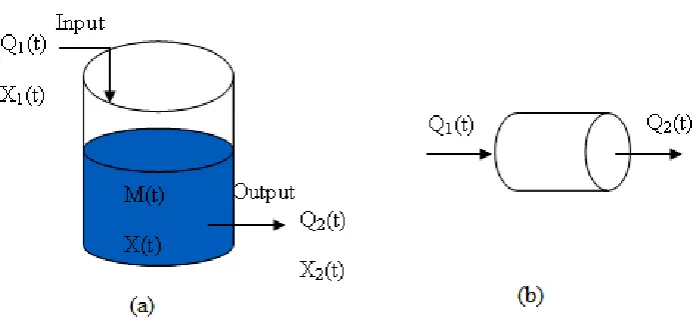
The general form of the dynamic population balance model of a reactor (such as the one
illustrated in Fig. 1) could be written as equations (1) and (2) in which mass variations per time unit (accumulation) within the reactor are related to its input, output and generation due to the reactions [18]. M(t) stands for the total mass of the material within the reactor at any time t; Q1(t) and Q2(t) are instantaneous input and output flow rates; X(t), X1(t) and X2(t) are the concentrations of the desired component (e.g. gold in solids ) inside the reactor, in the input and output flow rate of the reactor, respectively. P(t), also known as production flow rate (or generation), is equal to the mass of the desired component produced (or consumed) per time unit due to a chemical or physical reaction.
The term P(t) varies depending on the definition of the system, its components and the order of reactions. For instance, if X(t) is defined as the concentration of gold in solids and the reaction is a first-order leaching process, P(t)
would be M(t)*R(t) in which R(t), the rate of the leaching reaction, could be written as k*X(t)
where k is the rate constant. If the reaction is second-order, R(t) would be k*X(t)2. If the reaction is a first-order grinding, X(t) can be defined as the fraction of particles retaining in a certain size class (e.g. Xi(t) for size fraction i) and P(t) can be defined as mass variations of particles in the size fraction i due to the physical reaction of grinding. Such a reaction consists of deportation of particles from this class (expressed by –Si*Xi(t)*M(t) in the model) and deportation of particles into this class due to breakage of coarser particles (expressed in the
model as 1
1
i
j ij j
j S b X t M t
) [19]. Thesame approach can be applied to the modeling of flotation process. Population balance modeling has been applied and validated by different researchers to model the dynamic behavior of grinding [19], leaching [20] and flotation [21]. In development of this simulator, the data from the subject’s literature were used for verification of the simulator, which is discussed later.
) ( ) ( / )
(t dt Q1 t Q2 t
dM (1)
( ) ( ) / ( ) ( )
( ) ( ) ( )
dM t X t dt Q t X t
Q t X t P t
1 1
2 2
(2)
Fig. 1. A schematic reactor: a) a dynamic system, b) a non-dynamic system
If neither mass accumulation is supported by the system nor the materials residence time in the reactor is noticeable, the reactor will not act as a dynamic system; i.e. input variations have an instantaneous effect on the system’s output. A short pipe filled with incompressible fluid (Fig. 1b) is an example of such a system in which flow rate variations in one side of the pipe is observed instantly on its other side, as the residence time is very short (negligible) and no accumulation can occur in the system. In this paper, the output of such systems as crushers and hydrocyclone is calculated at any given time based on input values at the same time using the steady-state models. This helps disregard the insignificant residence time of the particles in the system. For systems with no accumulation and no mixing processes, but with significant residence time of particles, time delays were considered in addition to steady-state models (as in belt conveyors). Withen’s model for crushers [22], Karra’ model for screens [23] and a conceptual model for hydrocyclones [24] were applied in this study based on such an analogy.
2.2. Simulator development
2.2.1. Simulator structure
The population balance modeling approach is ideally suited to the needs of a plant simulator since it is comparatively simple for the products of any unit model to become the feed material for another unit [25]. The graphical block diagram representation of units in Simulink, in which every unit receives the output of another unit as its input, facilitates the plant-wide simulation using population
balance models. Particularly, since our models are defined as differential equations that need to be solved, Matlab/Simulink provides an excellent simulation environment that not only facilitates circuit design through its visual selection and linking of unit blocks, but also the built-in solvers of Matlab handle the differential equations of the models.
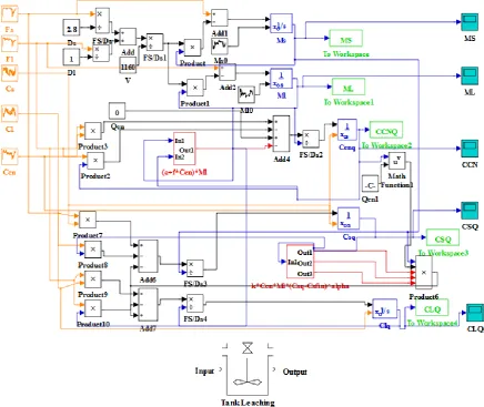
Figure 2 shows how the differential equation model of leaching (presented in Appendix B) [20] is imported into the Simulink environment. Variables are described in Appendix B, while Fs and Fl of Figure 2 are Qs(t) and Ql(t) of the model. k, e, f, alpha and Csfin are parameters of the model. The whole model is then masked under a leaching icon to build the leaching simulator block. Similarly, simulation blocks of other pieces of equipment were also developed and all were emplaced in a library (Fig. 3). In addition to basic equipment, some accessories (such as sump, conveyor belt, and PID control block) that were needed to form a circuit were also included in this library. Each block consisted of input and output streams, to get connected to other blocks.
Khoshnam et al. / Int. J. Min. & Geo-Eng., Vol.49, No.1, June 2015
including the mass flow rate of the solid input, solid density, mass flow rate of the liquid input, liquid density, mineral concentration in liquid (ppm), reactant concentration in liquid (ppm), feed particle size distribution (%), mineral grade in solid in each size class (%),
etc. By emplacing this block at the beginning of the circuits, the flow matrix can be transferred between the unit blocks, and the relevant entries of the matrix would change while passing through the equipment.
Fig. 2. Transfer of differential equations of dynamic leaching model to Simulink and making the “Tank Leaching” block
2.2.2. Integration of comminution and concentration
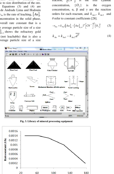
The grinding circuit can be connected to the concentration and extraction sections (leaching and flotation, in this research) by two different approaches. The first method requires an estimation of liberation characteristics of the ground ore and then employing those data in certain leaching or flotation models which include the liberation characteristics [26, 27]. The second approach, which is applied in this simulator, does not include the liberation directly, however
empirical models used to correlate the leaching kinetic to size distribution of the ore. For instance, Equations (3) and (4) are introduced by de Andrade Lima and Hodouin (2005) where rAu is the rate of leaching,
Au
s is the gold concentration in the solid phase,Au
k
is the overall rate constant that is a function of the average particle size of a size fraction,
Au s,shows the refractory goldconcentration (not leachable) that is also a function of average particle size of a size
fraction,
CN
is the free cyanideconcentration, [
O
2] is the oxygen concentration, α, β and γ are the reaction orders for each reactant, andk
Au1,k
Au2 andθ refer to constant coefficients [28].
,( )
Au Au s s
r k Au Au CN O
2 (3)
d
k
k
k
Au
Au1
Au2 (4)Fig. 3. Library of mineral processing equipment
Khoshnam et al. / Int. J. Min. & Geo-Eng., Vol.49, No.1, June 2015
2.3. Application of the simulator
With the help of Simulink GUI, a flowsheet could be developed only by dragging the desired equipment from the library (Fig. 3) and dropping them on the new blank sheet and connecting them by the lines. Operational variables of the equipment (such as flow rate and solid percentage) and parameters of the equipment model (such as dissolution rate constant, selection and breakage function) could be introduced to the blocks by simply double clicking on any equipment, which opens the developed data entry forms. Step, Ramp, Sinus or combination of them could be added to the any part of the circuit as a disturbance. The PID control block is also included in the library and could be added to the flowsheet.
3. Results and discussion
3.1. Verification of the simulator
Two different approaches were applied for verifying the simulator blocks. Blocks for which the dynamic data were available in the literature (such as leaching section) were verified by comparing the dynamic response of the simulator with the dynamic results from the literature. However, in a dynamic simulation, when all input variables are considered to be constant over time, the final results must be equal to the steady-state simulations. Additionally, if the input and output streams of a dynamic system are zero, it represents a batch system. Therefore, when no continuous dynamic data were available, the steady-state or batch performance of the
dynamic block was compared to the results from simulations using steady-state simulators such as Modsim (trial version), or batch dynamic data from the literature. Table 1 presents the references whose data were used for simulator verification.
Table 1. References used for verification of equipment blocks
Literature Equipment
Rajamani [19] Ball Mill
Whiten [22] Cone Crusher
Conceptual Model [24] Hydrocyclone
Lima [20] Leaching Tank
Adel and Luttrell [21] Mechanical flotation cell
Karra [23] Screen
Conradie [29] Sump
[30] Conveyor belt
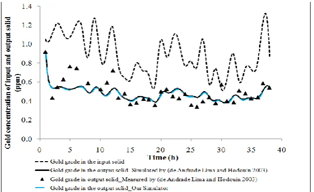
The leaching simulator block verification process is presented here as an example. Dynamic data used for verification of the leaching simulator were extracted from [20]. These included the gold concentration in both liquid and solid phases, solid flow rate and solid percentage measured at the entrance of an industrial leaching tank for 38 hours. Figure 5 shows the results of dynamic simulation of gold concentration at the tank outlet using the developed leaching block compared to the simulations done by [20]. Complete conformation of the results indicates the correct transfer of models into the Simulink environment.
3.2. Simulation of plant response to disturbance models (open loop)
Any disturbance model (step, impulse, and so on) could be easily implemented into the feed of any block; including the changes in particle size, composition distribution (grade of size fractions), solid percentage, hardness of the ore (by changing the selection function), kinetics of leaching or flotation and so on.
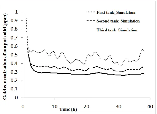
3.2.1. Leaching tanks in series
The simulated tank in Figure 5 is the first tank in a series of three tanks in the gold processing plant of Doyon mine, Quebec, Canada. The measured gold grade variations in the solid feed of the first tank are depicted in Figure 5, and the simulated gold grade variations in the output of the first tank are also presented. With the application of the developed simulator, the output of the second and third
tanks were simulated and presented in Figure 6. As it could be seen, although the variance of the disturbances of the gold grade in the input of the first tank was quite high, the long residence time of particles inside the tanks dampened the magnitude of the disturbances, and the variance of the disturbances of gold grade in output solids of tank 3 was very low. Such predictions about the quality of waste materials of the plant can be only available through dynamic simulation of the process and can improve the design of the circuit by introducing new criteria such as expected disturbances. Moreover, determining the amount of variations in each part of the circuit helps make better decisions for control strategies. The dampening effect of tank in series is one of the desirable outputs of such systems and, as it is discussed in next section, there are also other advantages.
Fig. 6. Prediction of wasted gold disturbances at the output of the plant
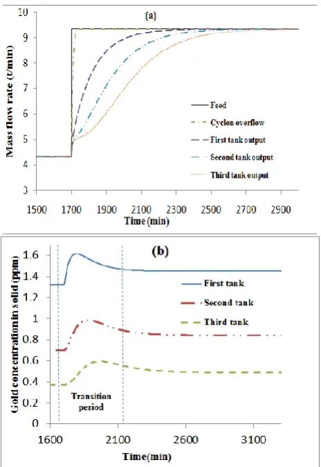
3.2.2. Integrated simulation of grinding and leaching
As an example, the dynamic simulation of a flowsheet, which integrates the grinding and leaching sections, is discussed here. The simulated circuit is given in Figure 7, where a step change in the solid flow rate of the plant feed (from 4.33 t/min to 9.33 t/min) is introduced at the time 1700 min, and the dynamic behavior of the circuit is analyzed. As it is shown in Figure 8a, although it takes less than 40 minutes for the grinding circuit to be stabilized at the new level of the flow rate, the final output of the plant reaches the new
Khoshnam et al. / Int. J. Min. & Geo-Eng., Vol.49, No.1, June 2015
and leaching tanks and the rate of reaching the new flow rate level causes a transition period in which the residence time in grinding and leaching tanks become even smaller than the final new level, leading to gold losses up to a peak of 0.59 ppm in around 2000 minutes. The
average gold loss in the transition period of 1700-2200 minutes is around 0.53 ppm, 0.04 ppm more than the finally stabilized 0.49 ppm; i.e. around 130 g of gold. This loss can be effectively reduced if a controller reduces the transition period.
Fig. 7. The simulation of integrated grinding and leaching circuit by the developed Simulink library
4. Conclusion
In this research, a dynamic simulator for mineral processing circuits was developed in Simulink environment. Phenomenological models based on the population balance methodology were used. The grinding circuit was connected to the concentration and extraction sections (leaching and flotation) using empirical models that correlate the leaching or flotation kinetic rates to the input particle size distribution. As an example, the dynamic behavior of a circuit containing grinding and leaching sections was simulated. It was shown that the dynamic response of the circuit can be substantially different for grade and throughput, causing transition periods with increased losses in valuable metals. Such predictions on metal content of streams are vital for control purposes, considering the inability of hard sensors for such online measurements and also considering the long residence time of the processes, causing delays in control actions. Additionally, the dampening effect of the number of tanks in series on waste grade disturbances was observed, and it was deduced that such simulations can be used to investigate some stability indices of the circuit, to be applied together with steady-state optimized criteria in design purposes.
References
[1] Aström, K.J., & Murray, R.M. (2010). Feedback systems: an introduction for scientists and engineers. Princeton university press.
[2] Hodouin, D. (2011). Methods for automatic control, observation, and optimization in mineral processing plants. Journal of Process Control,
21(2), 211225. doi:
http://dx.doi.org/10.1016/j.jprocont.2010.10.016.
[3] Liu, Y., & Spencer, S. (2004). Dynamic
simulation of grinding circuits. Minerals
Engineering, 17(11–12), 1189-1198. doi:
http://dx.doi.org/10.1016/j.mineng.2004.05.018.
[4] Hodouin, D., Dubé, Y., & Lanthier, R. (1988). Stochastic simulation of filtering and control strategies for grinding circuits. International Journal of Mineral Processing, 22(1–4),
261-274. doi:
http://dx.doi.org/10.1016/0301-7516(88)90068-3.
[5] Asbjörnsson, G., Hulthén, E., & Evertsson, M. (2013). Modelling and simulation of dynamic
crushing plant behavior with
MATLAB/Simulink. Minerals Engineering, 43–
44(0), 112-120. doi:
http://dx.doi.org/10.1016/j.mineng.2012.09.006.
[6] Hulthén, E., & Evertsson, C.M. (2009). Algorithm for dynamic cone crusher control. Minerals Engineering, 22(3), 296-303. doi: http://dx.doi.org/10.1016/j.mineng.2008.08.007.
[7] Asbjörnsson, G. (2013). Modelling and
Simulation of Dynamic Behaviour in Crushing Plants. PhD thesis, Chalmers University of Technology.
[8] Sbâarbaro, D. & Villar, R. del. (2010). Advanced Control and Supervision of Mineral Processing Plants. Springer.
[9] Asbjörnsson, G., Hulthén, E., & Evertsson, M. (2012). Modelling and dynamic simulation of gradual performance deterioration of a crushing circuit – Including time dependence and wear. Minerals Engineering, 33(0), 13-19. doi: http://dx.doi.org/10.1016/j.mineng.2012.01.016.
[10] Hulthén, E. (2010). Real-time
optimization of cone crushers. Chalmers University of Technology.
[11] Kianinia, Y., Khalesi, M.R., Khodadadi,
A., & Froutan, A. (2012). Designing Dynamic
Simulator of Grinding Circuit using
SIMULINK. Iranian Journal of Mining
Engineering, 7(17), 41-49.
[12] Khoshnam, F., Khalesi, M.R., & Zarei, M.J. (2013). Dynamic simulation of discharge of overflow mills based on mass balance equations in time and frequency domain. First International Conference on Mining, Mineral Processing, Metallurgical and Environmental Engineering, University of Zanjan.
[13] Zarei, M.J., Khalesi, M.R., & Khoshnam, F. (2013). Prediction of ball size variation effect on the output size distribution of mill by
dynamic simulation of grinding. First
International Conference on Mining, Mineral Processing, Metallurgical and Environmental Engineering, University of Zanjan.
[14] Hodouin, D., et al. (2000). Feedforward– feedback predictive control of a simulated flotation bank. Powder Technology, 108(2–3), 173-179. doi: http://dx.doi.org/10.1016/S0032-5910(99)00217-X.
[15] Pomerleau, A., et al. (2000). A survey of
grinding circuit control methods: from
decentralized PID controllers to multivariable
predictive controllers. Powder Technology,
108(2–3), 103-115. doi:
Khoshnam et al. / Int. J. Min. & Geo-Eng., Vol.49, No.1, June 2015
[16] Radhakrishnan, V.R. (1999). Model based
supervisory control of a ball mill grinding circuit. Journal of Process Control, 9(3),
195-211. doi:
http://dx.doi.org/10.1016/S0959-1524(98)00048-1.
[17] Yahyaee, M., & Banisi, S. (2004). How to control the level of column flotation cell in pilot plant of Sarcheshmeh. The conference of mining engineering of Iran, Tehran, Tarbiat Modares.
[18] Luyben, W. (1990). Process modeling,
simulation, and control for chemical engineers. McGraw-Hill chemical engineering series.
[19] Rajamani, R.K., & Herbst, J.A. (1991). Optimal control of a ball mill grinding circuit—I.
Grinding circuit modeling and dynamic
simulation. Chemical Engineering Science, 46(3), 861-870. doi: http://dx.doi.org/10.1016/0009-2509(91)80193-3.
[20] de Andrade Lima, L.R., & Hodouin,
D.(2003). Online Optimization of a Gold Extraction Process. in Control and Automation,
ICCA'03. Proceedings. 4th International
Conference on. 2003: IEEE.
[21] Adel, G.T., & Luttrell, G.H. (1999). An advanced control system for fine coal flotation. US Department of energy-contract DE-AC22-95PC95150.
[22] Whiten, W. (1972). The simulation of
crushing plants with models developed using multiple spline regression. Journal of the Soutf African Institute of Mining And Metallurgy, 257-264.
[23] Karra, V. (1979). Development of a model
for predicting the screening performance of a vibrating screen. Cim Bulletin, 72 167-171.
[24] Darling, P. (2011). SME Mining
engineering handbook. Vol. 1. SME.
[25] King, R.P. (2001). Modeling and
simulation of mineral processing systems. Access Online via Elsevier.
[26] Khalesi, M.R., et al. (2009). A liberation model for the integrated simulation of grinding and leaching of gold ore. in World Gold Conference 2009., The Southern African
Institute of Mining and Metallurgy:
Johannesburg, South Africa, 61-73.
[27] Khalesi, M.R., et al. (2011). Modelling of
the Gold Content within the Size Intervals of a Grinding Mill Product. in World Gold Conference 2011. Montreal, Canada.
[28] de Andrade Lima, L.R., & Hodouin, D. (2005). A lumped kinetic model for gold ore cyanidation. Hydrometallurgy, 79(3), 121-137. doi: http://dx.doi.org/10.1016/j.hydromet.2005.06.001.
[29] Conradie, A., & Aldrich, C. (2001). Neurocontrol of a ball mill grinding circuit using evolutionary reinforcement learning. Minerals
engineering, 14(10), 1277-1294. doi:
http://dx.doi.org/10.1016/S0892-6875(01)00144-3
[30] Itävuo, P., et al., (2013). Dynamic modeling and simulation of cone crushing circuits. Minerals
Engineering, 43–44(0), 29-35. doi:
Appendix A The model of ball mill (assuming to be one perfect mixer) [19]:
: Mass hold up
, : Mass fraction of material in the ith size interval in input and output
, : Mass rate of solids flow into and discharge from the mill
: Selection function for the ith size interval
: Breakage function,
Appendix B
The model of tank leaching (assuming to be one perfect mixer) [20]:
i: The number of tank
, : Ore and liquid mass hold up
, : Ore and liquid flow rate
: Gold concentration in the ore
: Gold concentration in the liquid
: Cyanide concentration in the liquid
: Rate of gold dissolution