The Thirty-Third AAAI Conference on Artificial Intelligence (AAAI-19)
Tensorial Change Analysis Using Probabilistic Tensor Regression
Tsuyoshi Id´e
IBM Research, Thomas J. Watson Research Center [email protected]
Abstract
This paper proposes a new method for change detection and analysis using tensor regression. Change detection in our set-ting is to detect changes in the relationship between the input tensor and the output scalar while change analysis is to com-pute the responsibility score of individual tensor modes and dimensions for the change detected. We develop a new prob-abilistic tensor regression method, which can be viewed as a probabilistic generalization of the alternating least squares al-gorithm. Thanks to the probabilistic formulation, the derived change scores have a clear information-theoretic interpreta-tion. We apply our method to semiconductor manufacturing to demonstrate the utility. To the best of our knowledge, this is the first work of change analysis based on probabilistic tensor regression.
Introduction
Change detection in temporal data has a variety of appli-cations across many industries. Depending on the specific type of data and changes expected, a number of different machine learning tasks can be defined. Of particular impor-tance is change detection in the supervised setting, whose goal is to detect a change in the relationship between the input and output variables. By analyzing the nature of the detected change in terms of controllable input variables, we can obtain actionable insights into the system.
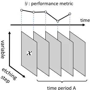
In the supervised setting, change detection has been treated typically as a regression problem. For a recent comprehensive review from an application perspective, see (Ge et al. 2017). As a natural extension of conventional vector-based regression approaches, condition-based mon-itoring based on tensor regression has attracted recent at-tention (Zhu, He, and Lawrence 2012; Fanaee-T and Gama 2016). As a real-world example, Fig. 1 illustrates the etch-ing process in semiconductor manufacturetch-ing. One etchetch-ing round consists of many, say 20, etching steps (chemical gas introduction, plasma exposure, etc.) and each of the steps is monitored with the same set of sensors (pressure, temper-ature, etc.), resulting in a two-way tensorX as the input. Note that neitherynorX is constant even under the normal condition due to different production recipes, random fluc-tuations, aging of the tool, etc. After etching, semiconductor
Copyright c2019, Association for the Advancement of Artificial Intelligence (www.aaai.org). All rights reserved.
vari
able
time : performance metric
time period A
Figure 1: Illustration of industrial change analysis using ten-sor regression in semiconductor etching. A scalary repre-senting the goodness of etching is predicted as a function of etching trace dataXin a tensor format. How can we quanti-tatively compare the time period A with a “golden period”?
wafers are sent to an inspection tool, which gives each of the wafers a scalaryrepresenting the goodness of etching.
When monitoring the process, imagine that we observed an unusual trend inyfor a certain time period (“time period A” in the figure). In order to get insights into how to fine-tune process parameters, we need to knowhowthe current situation is different from a “golden period”, in which ev-erything looked in good shape, in terms of the relationship betweenX andy. This is indeed a motivating example of theregression-based tensorial change analysis.
For practical change analysis, three major requirements should be met. First, obviously, a change analysis model must be able to quantitatively explain which tensor modes and dimensions contribute most to the changes detected. Second, it must be built on a probabilistic model between
X andy. The input tensor generally includes different phys-ical quantities. To make them comparable on the same ground, change scores should be formalized information-theoretically. Third, the change scores must be efficiently computed in both the training and testing phases.
regres-sion. Our tensor regression model can be viewed as a Bayesian re-formulation of the conventional alternating least squares (ALS) algorithm (Signoretto et al. 2014; Yu and Liu 2016; Zhou, Li, and Zhu 2013; Zhu, He, and Lawrence 2012). Although exact Bayesian inference is not possible, we derive an iterative inference algorithm using a varia-tional expectation-maximization framework (Tzikas, Likas, and Galatsanos 2008). Our contribution is the first proposal of (1) a Bayesian extension of ALS for tensor regression and (2) information-theoretic tensorial change analysis us-ing probabilistic tensor regression.
Related work
There are two categories of related work: tensorial change detection and probabilistic tensor regression models.
For the former, although much work has been done in se-quential tensor tracking using tensor factorization (Sun et al. 2008; Dunlavy, Kolda, and Acar 2011; de Araujo, Ribeiro, and Faloutsos 2017), most of them are based on the unsuper-vised setting. Little is known about the superunsuper-vised setting, especially information-theoretic approaches to performing both change detection and analysis.
For the latter, unlike tensor factorization, which has been a major research topic in machine learning for years, ten-sor regression is relatively new. For probabilistic tenten-sor re-gression, two major approaches can be found in the litera-ture: kernel methods and non-kernel methods. For the for-mer, most of the existing studies attempt to extend Gaus-sian process regression (GPR) for tensors (Zhao et al. 2014; Hou, Wang, and Chaib-draa 2015; Suzuki 2015; Kana-gawa et al. 2016; Imaizumi and Hayashi 2016). It may look straightforward to mechanically use the well-known formula of GPR (Rasmussen and Williams 2006), assum-ing that a kernel function between tensors is given. How-ever, the tricky part is that naive distance metrics such as
kX(n)−X(n0)k2
F, wherek·kFis the Frobenius norm, do not properly preserve structural information of tensors because they are reduced to the summation of the element-wise dis-tance, giving exactly the same expression as the naive vec-torized formulation.
To handle this issue, Zhao et al. (2014) and Ho et al. (2015) proposed to use a kernel func-tion defined through mode-wise matricizafunc-tion. Kana-gawa et al. (2016) considered GPR for the individual tensor modes l = 1, . . . , M and combine them for predicting
y. A similar approach was also used in (Suzuki 2015; Imaizumi and Hayashi 2016). For real-world industrial applications, however, these methods have significant limitations because, unlike the proposed Bayesian ALS, they need either Monte Carlo (MC) sampling on training or expensive computation of tensor factorization on testing.
For the non-kernel methods, only a limited number of studies is found in the literature. One of the earliest studies is Goldsmith et al. (2014) but it is based on a few strong as-sumptions specific to 3D imaging. Recently, Guhaniyogiet al.(2017) proposed a fully Bayesian tensor regression model with variable selection, using the CP (canonical polyadic) decomposition assumption for the regression coefficients.
As a result of its multi-layered hierarchical model with a fully Bayesian treatment, however, their model requires MC sampling for inference, making practical implementa-tion hard especially in the context of change analysis. Also, mainly due to the complexity of the model, how it is related to the existing alternating least squares and other regression work is not necessarily clear. In contrast, in the proposed probabilistic model all the steps for inference have a simple analytic expression thanks to a variational approximation. To the best of our knowledge, this is the first work to use a variational inference approach for tensor regression.
Tensor notations
We follow Kolda and Bader (2009) for most of the tensor notations. We denote (column) vectors, matrices, and ten-sors by bold italic (x, etc.), sanserif (A, etc.), and bold calli-graphic (X, etc.) letters, respectively. The elements of them are typically denoted by corresponding non-bold letters with a subscript (xi,Ai,j,Xi1,...,iM, etc.). We may also use[·]as the operator to select a specific element ([w]i ≡ wi, etc.), with≡being used to define the left hand side (l.h.s.) by the right hand side (r.h.s.). To simplify the notation, we may use non-italic bold letters to collectively represent the indexes of theM modes asi= (i1, . . . , iM). Superscripts are used to distinguish the tensor modes such asal.
The inner product of two same-sized tensors X,A ∈ Rd1×···×dMis defined as
(X,A)≡ X
i1,...,iM
Xi1,...,iMAi1,...,iM. (1)
The outer product between vectors is an operation to cre-ate a tensor from a set of vectors. For example, the outer product ofa1∈Rd1,a2∈
Rd3,a3∈
Rd3 makes a 3-mode
tensor ofd1×d2×d3dimension as
[a1◦a2◦a3]i1,i2,i3 =a
1 i1a
2 i2a
3
i3. (2)
The inner product between a tensor and a rank-1 tensor plays a major role in this paper. For example,
(X,a1◦ · · · ◦aM) = X
i1,...,iM
Xi1,...,iMa
1 i1· · ·a
M iM. (3)
This can be viewed as a “convolution” of a tensor by a set of vectors. Them-mode product is an operation to convolute a tensor with a matrix as
[X ×mS]i1,...,jm,...,iM ≡
dm X
im=1
Xi1,...,im,...,iMSjm,im. (4)
Tensorial Change Analysis Framework
This section summarizes the problem setting and tensorial change detection framework at a high level.
Problem setting
We are given a training datasetDconsisting ofNpairs of a scalar target variableyand an input tensorX:
where the superscript in the round parenthesis is used to de-note the n-th sample. Both the input tensor and the target variable are assumed to becentered.X(n)’s haveM modes in which thel-th mode hasdldimensions.
We assume a linear relationship asy∼(A,X), in which the coefficient tensor follows the CP expansion of orderR:
A=
R X
r=1
a1,r◦a2,r◦ · · · ◦aM,r. (6)
Using a probabilistic model described in the next subsec-tion, our first goal is to obtain the predictive distribution
p(y | X,D)for an unseen sampleX, based on the poste-rior distribution for{ar,l}and the other model parameters learned from the training data.
Change analysis scores
We give the definition of change scores for three sub-tasks in tensorial change analysis: Outlier detection, change de-tection, andchange analysis.
First, the outlier score is defined for a single pair of obser-vation(y,X)to quantify how much uncommon they are in reference to the training data. Given the predictive distribu-tionp(y|X,D), we define the outlier score as the logarith-mic loss (Yamanishi et al. 2004):
c(y,X)≡ −lnp(y|X,D)
={y−µ(X)}
2
2σ2(X) +
1 2ln{2πσ
2(
X)}, (7)
where the second line follows from the explicit from ofp(y|
X,D)given later (Eq. (40)).
Second, we define the change-point score by averaging the outlier score over a setD˜:
c( ˜D,D) = 1 ˜
N X
n∈D˜
c(y(n),X(n)), (8)
whereN˜ is the sample size ofD˜. The setD˜ is typically fined using a sliding window for temporal change-point de-tection.
Third, for change analysis, we leverage the posterior distribution of the CP-decomposed regression coefficient
{al,r}. As shown in the next section, the posterior distribu-tion, denoted asq1l,r(al,r), given by a Gaussian distribution:
ql,r1 (al,r) =N(al,r|µl,r,Σl,r), (9)
where the first and second arguments after the bar repre-sents the mean and the covariance matrix, respectively. As explained in Fig. 1, the goal of change analysis is to quantify the contribution of each tensorial mode to the distributional difference between two datasets, say D,D˜. For the (l, r) -mode, this can be calculated as the Kullback-Leibler (KL) divergence ofq1l,r(al,ri |al,r−i), the conditional distribution for
thei-th dimension given the rest:
cli( ˜D,D)≡
1
R
R X
r=1 Z
dal,rq1l,r(al,r) lnq
l,r 1 (a
l,r i |a
l,r
−i)
˜
ql,r1 (al,ri |al,r−i)
= 1 2R
R X
r=1 (
[˜Λl,r( ˜µl,r−µl,r)]2 i
˜
Λl,ri,i + ln Λl,ri,i
˜
Λl,ri,i
+ [˜Λ
l,r
Σl,rΛ˜l,r]i,i
˜
Λl,ri,i −1
)
(10)
where the tilde ˜ specifies the model learned on D˜ and
Λl,r ≡(Σl,r)−1etc., whose explicit form is given later (see Eq. (22)).
Note that in the above definitions the capability of produc-ing probabilistic output is critical. Also, they can be straight-forwardly computed without any expensive computations such as tensor factorization and MC sampling.
Probabilistic model for tensor regression
This section derives the inference algorithm of the proposed probabilistic tensor regression model.
Observation model and priors
Our probabilistic tensor regression model consists of only two primary ingredients: an observation model to describe measurement noise and a prior distribution to represent the uncertainty of regression coefficients.
First, the observation model for the centered data is de-fined as
p(y |X,A, λ) =N(y|(A,X), λ−1), (11) whereN(y | ·,·)denotes the univariate Gaussian distribu-tion with the mean(A,X)and the precisionλ.
Second, for the prior distribution of the coefficient vectors al,r, we use the Gauss-gamma distribution as
p({al,r}) =
M Y
l=1 R Y
r=1
N(al,r|0,(bl,r)−1Idl), (12)
p(bl,r|α0, β0) =G(α0, β0)≡
β0α0
Γ(α0)
(bl,r)α0−1e−β0bl,r
(13)
where Idl is the dl-dimensional identity matrix and Γ(·) is the gamma function. The hyper-parameters α0, β0 are assumed to be given. Note that the parameter λ is deter-mined as part of learning and there is no need for cross-validation. This is one of the advantages of probabilistic for-mulation and is in contrast to the existing frequentist tensor regression work (Signoretto et al. 2014; Yu and Liu 2016; Zhou, Li, and Zhu 2013; Zhu, He, and Lawrence 2012).
Variational inference strategy
point-estimated parameters. Then, given the posterior just estimated, the variational M (VM) step point-estimates the parametersλby maximizing the posterior expectation of the log complete likelihood. The log complete likelihood of the model plays the central role here:
L(A,b, λ) = c.+1 2
N X
n=1 n
lnλ−λ∆(y(n),X(n))2o
+
M X
l=1 R X
r=1
1 2dllnb
l,r−1
2b
l,rkal,rk2 2
+
M X
l=1 R X
r=1
(α0−1) lnbl,r−β0bl,r , (14)
wherec.is a symbolic notation for an unimportant constant,
k · k2is the 2-norm, andbis a shorthand notation for{br,l}. We also defined
∆(y,X)≡y−
R X
r=1
(X,a1,r◦ · · · ◦aM,r), (15)
where we have omitted the dependency onAon the l.h.s. for simplicity.
VE step: Posterior for coefficient vectors
The VB step finds an approximated posterior in a factorized form. In our case, we seek a VB posterior in the form
Q({al,r, bl,r}) =
M Y
l=1 R Y
r=1
q1l,r(al,r)q2l,r(bl,r). (16)
The distributionsq1l,r, q2l,rare determined so that they min-imize the KL divergence from the true posterior. The key fact here is that the true posterior is proportional to the com-plete likelihood by Bayes’ rule. Thus, the KL divergence is represented as
KL = c.+hlnQi − hL(A,b, λ)i,
whereh·irepresents the expectation with respect toQ. Here the unknowns are not variables but functions. However, according to calculus of variations (see e.g. Appendix D in (Bishop 2006)), roughly speaking, we can formally take the derivative with respect to q1l,r or q2l,r and equate the derivatives to zero. In that way, the condition of optimality is given by
VE step: lnq1l,r(al,r) = c.+hL(A,b, λ)i\al,r, (17)
lnq2l,r(bl,r) = c.+hL(A,b, λ)i\bl,r, (18)
where h·i\al,r and h·i\bl,r denotes the expectation with
Q/ql,r1 andQ/ql,r2 , respectively.
Now let us solve the first equation. Unlike the case of single-mode vector-based regression,L(A,b, λ)has a com-plex nonlinear dependency on{al,r}, especially in the term of ∆2. However, to compute h·i\al,r, we can leverage the
fact that each of theal,rs can be factored out in the inner product:
(X,a1,r◦ · · · ◦aM,r) = (al,r)>φl,r(X), (19)
where > denotes the transpose. The j-th element of φl,r(X)∈Rdlis defined by
[φl,r(X)]j≡ X
i1,...,iM
Xi1,...,iMδ(j, il) Y
m6=l
am,ri
m , (20)
whereδ(j, il)is Kronecker’s delta, which takes one only if
j=ilzero otherwise. Using this andµl,r≡ hal,ri, we have
h∆(y,X)2i\al,r = c.+al,r
>
hφl,rφl,r>ial,r
−2al,r>hφl,ri[y−X
r06=r
(X,µ1,r0◦ · · · ◦µM,r0)], (21)
wherec.is a constant not including theal,r andh·i with-out subscript denotes the expectation byQ(Eq. (16)). We dropped the subscript\al,r on the r.h.s. because φl,r does not include theal,r.
The VB equation (17) now looks like:
lnql,r1 (al,r) = c.−1
2a
l,r>(Σl,r)−1al,r+λal,r>Φl,ryl,r N ,
where
Σl,r≡
(
λ
N X
n=1
hφl,r,(n)φl,r,(n)>i+hbl,riI dl
)−1 (22)
Φl,r≡[hφl,r,(1)i, . . . ,hφl,r,(N)i] (23)
[yNl,r]n≡y(n)− X
r06=r
(X(n),µ1,r0◦ · · · ◦µM,r0), (24)
with φl,r,(n) being a shorthand notation for φl,r(X(n)) . Thus we conclude that ql,r1 (al,r) = N(al,r | µl,r,Σl,r
)
withΣl,rbeing Eq. (24) and
µl,r =λΣl,rΦl,ryl,rN. (25)
Usingq1l,r, we can explicitly computehφl,rφl,r>ias
[hφl,rφl,r>i]i,j= X
i,j
XiXjδ(i, il)δ(jl, j) Y
m6=l
Sim,r
m,jm,
(26)
Sm,r≡ ham,ram,r>i=Σm,r+µm,r(µm,r)> (27)
where we used the notation ofi = (i1, . . . , iM)etc. Sim-ilarly, hφl,riis given just by replacing am,r
im withµ m,r im in Eq. (23).
The posterior mean (25) has clear similarities with ordi-nary least squares. Foral,r, the vectorφl,r acts as the pre-dictor and Φcan be interpreted as the data matrix. Also, given the otherµl,r0 (r0 6=r), the vectoryl,r
VE step: Posterior for
{
b
l,r}
Now let us consider the second VE equation (18). Arranging the last terms ofLin Eq. (14), we have
lnq2l,r(bl,r) = c.+ (αl,r−1) lnbl,r−βl,rbl,r,
αl,r≡α0+
1
2dl (28)
βl,r≡β0+
1 2Tr(Σ
l,r
) +kµl,rk2
2 (29)
which leads to the solution
q2l,r(bl,r) =G(bl,r |αl,r, βl,r), (30) whereGdenotes the Gamma distribution defined in Eq. (13). Using this we can computehbl,riin Eq. (22). By the basic property of the gamma distribution,
hbl,ri= α
l,r
βl,r =
dl+ 2α0
Tr(Σl,r) +kµl,rk2 2+ 2β0
, (31)
where we have used Eq. (27) for Eq. (29).
VM step: Point estimation of
λ
The next step of the vEM procedure is to point-estimateλ
by maximizing the posterior expectation of the log complete likelihood. Formally, our task is
VM step:λ= arg max
λ hL(A,b, λ)i. (32) To do this, we need an explicit representation of
hL(A,b, λ)i. Again, the most challenging part is to find the expression ofh∆2i. In this case, we do not need to factor out a specifical,r. By simply expanding the square, we have
h∆(y,X)2i=y2−2yX
r
h(X,a1,r◦ · · · ◦aM,r0)i
+X
r,r0
h(X,a1,r◦ · · · ◦aM,r)(a1,r0◦ · · · ◦aM,r0,X)i
=
(
y−X
r
(X,µ1,r◦ · · · ◦µM,r)
)2
+X
r
Γr(X),
where we usedham,ri
m a m,r jm i= [S
m,r
]im,jm to define
Γr(X)≡(X ×1S1,r×2· · · ×M SM,r,X)
−(X,µ1,r◦ · · · ◦µM,r)2. (33) The condition of optimality forλis now given by
0 = ∂hLi
∂λ = N
2λ−
1 2
N X
n=1
h∆(y(n),X(n))2i, (34)
resulting in
λ−1= 1
N
N X
n=1 (
y(n)−
R X
r=1
(X(n),µ1,r◦ · · · ◦µM,r)
)2
+ 1
N
N X
n=1 R X
r=1
Γr(X(n)) (35)
Algorithm 1Bayesian ALS (BALS) for Tensor Regression. Input:{(y(n),X(n))}N
n=1,R. Output:{µl,r,Σl,r, αl,r, βl,r}, λ.
Initialize: µl,r as random vector and hbil,r as 1 for
∀(l, r). repeat
λ−1←Eq. (35) forl←1, . . . , Mdo
forr←1, . . . , Rdo
Σl,r←nλPN
n=1hφl,r,(n)φl,r,(n) >
i+hbl,riI dl
o−1
µl,r←λΣl,rΦl,ryl,r N
βl,r←β
0+12Tr(Σl,r) +kµl,rk22 end for
end for untilconvergence
Although the multi-way nature of tensors makes things significantly complicated, this has a clear interpretation. SincehAi=PR
r=1µ
1,r◦ · · · ◦µM,r,the first term is the
same as the standard definition of the variance as the squared deviation from the mean. The second term comes from in-teractions between different modes.
Algorithm 1 summarizes the entire vEM inference pro-cedure, which we call the Bayesian ALS(BALS) for ten-sor regression, as this algorithm is most naturally viewed as a Bayesian extension of the ALS algorithm (see Propo-sition 1). Following (Kohn, Smith, and Chan 2001), we fix α0 = 1, β0 = 10−6 so the prior becomes near non-informative. The rankRis virtually the only input parameter to be tuned. Fore.g.anomaly detection,Rcan be determined by evaluating AUC (area under curve) of the ROC (receiver operating characteristic) curve for each ofR= 1,2,3, . . ..
Despite its seeming simplicity, implementing BALS is not necessarily straightforward. For actual implementation, it is advisable to use a few tensor algebraic tricks. It is also some-time useful to use mean-field-like approximations for nu-merical stabilities, as shown in the next subsection. The total complexity of the algorithm depends on the formulas to use and there is a subtle trade-off among codability, efficiency, numerical stability, and memory usage. We omit the details here for space limitations.
Relationship with classical ALS
Here we discuss the following proposition:
Proposition 1 The classical ALS solution is the maximum a posteriori (MAP) approximation of the Bayesian ALS.
To prove this, letbl,r = ρλ for a constantρ. The MAP solution is the one to maximize the log likelihood with re-spect to{al,r}. By differentiating Eq. (14), we easily get the condition of optimality
N X
n=1 (
y(n)−
R X
r0=1
(al,r0)>φl,r0,(n) )
which readily gives an iterative formula:
˜
Σl,r←
( N X
n=1
φl,r(X(n))φl,r(X(n))>+ρI
dl )−1
(36)
al,r←Σ˜l,rΦl,ryl,rN, (37)
where we used the same notations as the probabilistic coun-terpart (Eqs. (23) and (24)). To establish the relationship with the traditional notation of ALS, we note that Eq. (20) can be written as
φl,r=X(l)(aM,r⊗ · · · ⊗al+1,r⊗al−1,r⊗ · · · ⊗a1,r), (38)
where X(l) is the mode-l matricization of X (Kolda and Bader 2009) and⊗denotes the Kronecker product. With this identity, we conclude that the MAP solution is the equivalent to the classical ALS with the`2regularizer (see,e.g.(Zhou, Li, and Zhu 2013) for an explicit expression).
In comparison to the frequentist ALS solution, there are three major advantages of BALS. First, in the Bayesian ALS, the regularization parameter is automatically learned as part of the model. In ALS,ρhas to be cross-validated. Second, BALS can provide a probabilistic output, while the ALS has to resort to extra model assumptions for that. This is a significant limitation in many real applications, espe-cially when applied to change analysis. Third, in BALS, the alternating scheme is derived as a natural consequence of the factorized assumption of Eq. (16), in which the vEM frame-work provides a clear theoretical foundation of the whole procedure.
Predictive distribution
Using the learned model parameters and the posterior dis-tribution foral,r, we can build a predictive distribution to predictyfor an unseenX as
p(y|x,D) =
Z Y
l,r
dal,rq1l,r(al,r)N(y|(X,A), λ−1).
Due to the intermingled form of different modes, the exact integration is not possible despite the seeming linear Gaus-sian form. However, we can derive an approximated result in the following way. First, pick an arbitrary(l0, r0), and use the factored form Eq. (19). By performing integration with respect toal0,r0, we have
Z
dal0,r0q1l0,r0(al0,r0)N(y|(X,A), λ−1)
=N(y|µl0,r0>φl0,r0, λ−1+φl0,r0>Σl0,r0φl0,r0). (39)
To proceed to a next(l00, r00), we need to factor out theal00,r00 formφl0,r0. The problem is that the variance is a complex function ofal00,r00. Here, as an approximation, we replace
the variance withλ−1+ Tr(Σl0,r0
hφl0,r0φl0,r0>i)and take account of the dependency ofal00,r00only in the mean.
In this way, we obtain the predictive distribution as
p(y|x,D) =N(y|µ(X), σ2(X)) (40)
BALS n-GPR d-GPR
RMSE
0
50
100
150
BALS n-GPR d-GPR
total computation time [s]
0
10
20
30
40
50
Figure 2: Comparison of the RMSE and the total computa-tion time on average from training through testing.
with
µ(X) =η+
R X
r=1
(X,µ1,r◦ · · · ◦µM,r), (41)
σ2(X) =λ−1+
R X
r=1 M X
l=1
TrΣl,rhφl,rφl,r>i, (42)
whereη is to offset non-centered testing data. If we denote the sample average ofyandX overrawtraining samples by
¯
yandX¯, respectively,ηis given by
η ≡y¯−
R X
r=1
( ¯X,µ1,r◦ · · · ◦µM,r). (43)
Herehφl0,r0φl0,r0>iis given by Eq. (26). Unlike the GPR-based tensor regression methods (Zhao et al. 2014; Hou, Wang, and Chaib-draa 2015; Suzuki 2015; Kanagawa et al. 2016; Imaizumi and Hayashi 2016), we do not need any heavy computations of CP or Tucker decomposition upon testing.
Experiments
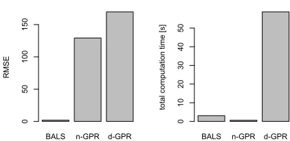
As discussed, the problem of tensorial change analysis is new and existing methods are not directly comparable about the change analysis part. Thus, we focus on 1) demonstrat-ing the practical utility of BALS in computdemonstrat-ing mode-wise change analysis scores for a real-world application. We also illustrate major features of BALS by 2) comparing with al-ternatives on metrics such as computational time.
In the present context, whose primary goal is to compute the information-theoretic change analysis score (10), two GPR-based models are relevant to BALS. One is based on the naive Gaussian kernelσ0e−kX−X
0k2
F/σ
2
, which we call n-GPR. The other is based on the state-of-the-art mode-wise kernel decomposition:σ0Q
M l=1e
−D(X(l),X0(l))/σ 2
,which we call d-GPR. HereD(·,·)a distance function between
0.0 0.2 0.4 0.6 0.8 1.0
0.2
0.4
0.6
0.8
1.0
1 - (normal sample accuracy)
abnormal sample accuracy
BALS n-GPR d-GPR
Figure 3: ROC curves for London School data with AUC values 0.96, 0.85, 0.88 for BALS, n-GPR, d-GPR, respec-tively.
0.0
2.0
outlier score
0 200 400 600 800 1000 1200 1400
0.2
0.5 change-point score
etch round index
Figure 4: Outlier and change-point scores (withN˜ = 50in Eq.(8)) for the semiconductor etching data.
Synthetic data
To show general features of BALS in comparison to the al-ternatives, we synthetically generated mode-3 (M = 3) ten-sor data in(d1, d2, d3) = (10,8,5)with a given set of the coefficients and randomly generated covariance matrices. For the covariance matrices, we first randomly generated the entries of matrices of the sizeRd1×d1,
Rd2×d2,
Rd3×d3
using the standard normal distribution and made them posi-tive definite by replacing the eigenvalues in their eigenvalue decomposition with random positive numbers sampled from
G(1,1/2). To be fair to n-GPR, which corresponds to the vectorized regression, and to simulate heavy fluctuations in the real-world, we added a t-distributed noise to a vector-ized representation and generated500samples. The param-eters are optimized using 5-fold cross-validation (CV), so the root mean squared error (RMSE) was minimized.
As summarized in Fig. 2, in spite of many outliers due to thet-noise, BALS outperformed the alternatives in RMSE. It is interesting that the GPR-based methods failed to cap-ture the underlying generative model even with the mode-decomposed GPR method. This is mainly because the ker-nel trick (Bishop 2006) does not guarantee the primal-dual equivalence for tensors withM ≥3. Figure 2 also compares the total computational time on average (for an optimal hy-perparameter choice) from training to testing (3.1, 0.6, 58.7 seconds from left to right). n-GPR is the fastest although BALS is comparable to it. Due to extra operations for matri-cization, d-GPR is much costlier than the others.
X12 X11 X10X9 X8 X7 X6 X5 X4 X3 X2 X1 D23 D22 D21 D20 D19 D18 D17 D16 D15 D14 D13 D12 D11 D10D9 D8 D7 D6 D5 D4 D3 D2 D1
score 0e+00 2e+07
mode 1 (variable)
14 13 12 11 10 9 8 7 6 5 4 3 2 1
score 0e+00 2e+07 4e+07
mode 2 (step)
Figure 5: Change analysis score showing the contribution of individual modes and dimensions.
0 200 400 600 800 1000 1200 1400
1000
3000
5000
etch round index
value
X12, 3rd step
Figure 6: Observed sensor values of X35,3, which corre-sponds to the most contributing dimension in Fig. 5.
London School data
Next, we tested outlier detection capabilities of BALS using publicly available London School data (Goldstein 1991) to pick unusually well-performing schools in the data cleans-ing task, in which schools whose median of ‘exam.score’ is greater than 25 are defined as outliers. We created 139
R4×5×2tensors by computing ‘% of FSM,’ the number of VR1 students, the number of VR2 students, and the school denomination for each pair of gender and ethnicity. The original eleven ethnicity groups were converted into five groups by merging the smallest groups. In BALS, we picked
R = 7that gave the maximum AUC value. Figure 3 com-pares ROC curves, which shows BALS outperforms the al-ternative in terms of AUC.
Semiconductor etching diagnosis
of (X, y), where X is a 35 (variables) × 14 (steps) ten-sor andyis a scalar performance metric. The testing dataset has1 372pairs and includes an excursion event towards the end of the observation period, in which the last 372 samples were assumed to be anomalous. Although human engineers successfully detected the excursion event semi-manually, the true root cause is unknown.
Figure 4 shows the outlier and change-point scores. We pickedR= 4that maximized AUC. In the figure, a clear in-crease of the score is observed towards the end, correspond-ing to the excursion event, which can be used for early warn-ing. Figures 5 shows the changeanalysisscore computed by Eq. (10), which shows a dominant contribution of the vari-ablex12and the third step. Figure 6 shows raw signal ofx12 in the third step. Very interestingly, this variable has a recog-nizable increase in the amplitude of fluctuation towards the end, suggesting a potential root cause of the excursion event.
Conclusion
We have proposed a new tensorial change analysis frame-work based on a newly developed probabilistic tensor re-gression algorithm, which can be viewed as a probabilistic generalization of the alternating least square algorithm. It can compute change scores for individual tensor modes and dimensions in an information-theoretic fashion, providing useful diagnostic information. To the best of our knowledge, this is the first work of variational Bayesian formulation of probabilistic tensor regression and information-theoretic formulation of tensorial change analysis in the supervised setting. Finally, we successfully applied our method to a change diagnosis task in semiconductor manufacturing.
References
Bishop, C. M. 2006. Pattern Recognition and Machine Learning. Springer-Verlag.
de Araujo, M. R.; Ribeiro, P. M. P.; and Faloutsos, C. 2017. Tensorcast: Forecasting with context using coupled tensors. In Proc. IEEE International Conference on Data Mining (ICDM), 71–80. IEEE.
Dunlavy, D. M.; Kolda, T. G.; and Acar, E. 2011. Temporal link prediction using matrix and tensor factorizations. ACM Transactions on Knowledge Discovery from Data5(2):10.
Fanaee-T, H., and Gama, J. 2016. Tensor-based anomaly de-tection: An interdisciplinary survey.Knowledge-Based Sys-tems98:130–147.
Ge, Z.; Song, Z.; Ding, S. X.; and Huang, B. 2017. Data mining and analytics in the process industry: the role of ma-chine learning.IEEE Access5:20590–20616.
Goldsmith, J.; Huang, L.; and Crainiceanu, C. M. 2014. Smooth scalar-on-image regression via spatial Bayesian variable selection. Journal of Computational and Graphi-cal Statistics23(1):46–64.
Goldstein, H. 1991. Multilevel modelling of survey data. Journal of the Royal Statistical Society. Series D (The Statis-tician)40(2):235–244.
Guhaniyogi, R.; Qamar, S.; and Dunson, D. B. 2017. Bayesian tensor regression. Journal of Machine Learning Research18(79):1–31.
Hou, M.; Wang, Y.; and Chaib-draa, B. 2015. Online local Gaussian process for tensor-variate regression: Application to fast reconstruction of limb movements from brain sig-nal. InProc. IEEE International Conference on Acoustics, Speech and Signal Processing (ICASSP), 5490–5494. Imaizumi, M., and Hayashi, K. 2016. Doubly decompos-ing nonparametric tensor regression. InProc. International Conference on Machine Learning, 727–736.
Kanagawa, H.; Suzuki, T.; Kobayashi, H.; Shimizu, N.; and Tagami, Y. 2016. Gaussian process nonparametric tensor estimator and its minimax optimality. InProc. International Conference on Machine Learning, 1632–1641.
Kohn, R.; Smith, M.; and Chan, D. 2001. Nonparamet-ric regression using linear combinations of basis functions. Statistics and Computing11(4):313–322.
Kolda, T. G., and Bader, B. W. 2009. Tensor decompositions and applications. SIAM review51(3):455–500.
Rasmussen, C. E., and Williams, C. 2006. Gaussian Pro-cesses for Machine Learning. MIT Press.
Signoretto, M.; Dinh, Q. T.; De Lathauwer, L.; and Suykens, J. A. 2014. Learning with tensors: a framework based on convex optimization and spectral regularization. Machine Learning94(3):303–351.
Sun, J.; Tsourakakis, C. E.; Hoke, E.; Faloutsos, C.; and Eliassi-Rad, T. 2008. Two heads better than one: pattern discovery in time-evolving multi-aspect data. Data Mining and Knowledge Discovery17(1):111–128.
Suzuki, T. 2015. Convergence rate of Bayesian tensor es-timator and its minimax optimality. InProc. International Conference on Machine Learning, 1273–1282.
Tzikas, D. G.; Likas, A. C.; and Galatsanos, N. P. 2008. The variational approximation for Bayesian inference.IEEE Signal Processing Magazine25(6):131–146.
Yamanishi, K.; Takeuchi, J.-I.; Williams, G.; and Milne, P. 2004. On-line unsupervised outlier detection using finite mixtures with discounting learning algorithms. Data Min-ing and Knowledge Discovery8(3):275–300.
Yu, R., and Liu, Y. 2016. Learning from multiway data: Sim-ple and efficient tensor regression. InProc. International Conference on Machine Learning, 373–381.
Zhao, Q.; Zhou, G.; Zhang, L.; and Cichocki, A. 2014. Tensor-variate Gaussian processes regression and its appli-cation to video surveillance. InProc. IEEE International Conference on Acoustics, Speech and Signal Processing (ICASSP),, 1265–1269. IEEE.