On-Line Learning of Linear Dynamical Systems: Exponential Forgetting in Kalman Filters

The Thirty-Third AAAI Conference on Artificial Intelligence (AAAI-19)

On-Line Learning of Linear Dynamical

Systems: Exponential Forgetting in Kalman Filters

Mark Kozdoba,

_{Jakub Marecek,}

_{Tigran Tchrakian,}

_{Shie Mannor}

[email protected], [email protected],[email protected], [email protected]

Abstract

The Kalman filter is a key tool for time-series forecasting and analysis. We show that the dependence of a prediction of Kalman filter on the past is decaying exponentially, whenever the process noise is non-degenerate. Therefore, Kalman filter may be approximated by regression on a few recent observa-tions. Surprisingly, we also show that having some process

noise isessentialfor the exponential decay. With no process

noise, it may happen that the forecast depends on all of the past uniformly, which makes forecasting more difficult. Based on this insight, we devise an on-line algorithm for im-proper learning of a linear dynamical system (LDS), which considers only a few most recent observations. We use our de-cay results to provide the first regret bounds w.r.t. to Kalman filters within learning an LDS. That is, we compare the results of our algorithm to the best, in hindsight, Kalman filter for a given signal. Also, the algorithm is practical: its per-update run-time is linear in the regression depth.

Introduction

Linear Dynamical Systems (LDS) are a key standard tool in modeling and forecasting time series, with an exceedingly large number of applications. In forecasting with an LDS, typically one learns the parameters of the LDS first, using a maximum likelihood principle, and then uses Kalman fil-ter to generate predictions. The two features that seem to contribute the most to the success of LDS in practice are the ability of LDS to model a wide range of behaviors, and the recursive nature of Kalman filter, which allows for fast, real-time forecasts via a constant-time update of the previous estimate. On the other hand, a major difficulty with LDSs is that the process of learning system parameters, via ex-pectation maximization (EM) or direct likelihood optimiza-tion, may be time consuming and prone to getting stuck in local maxima. We refer to (Anderson and Moore 1979; West and Harrison 1997; Hamilton 1994; Chui and Chen 2017) for book-length introductions.

Recently, there has been an interest in alternative, im-proper learning approaches, where one approximates the predictions of LDSs by a linear function of a few past obser-vations. The advantage of such approaches is that it convex-ifies the problem, i.e., learning the linear function amounts

Copyright c2019, Association for the Advancement of Artificial

Intelligence (www.aaai.org). All rights reserved.

to a convex problem, which avoids the issues brought by the non-convex nature of the likelihood function. The con-vexification allows for on-line algorithms, which are typi-cally fast and simple. A crucial advance of these recent ap-proaches is the guarantee that the predictions of the convex-ified, improper-learning algorithm are at least as good as the predictions of the proper one. One therefore avoids the long learning times and issues related to non-convexity associated with the classical algorithms, while maintaining the statisti-cal performance.

Leading examples of this approach (Anava et al. 2013; Liu et al. 2016; Hazan, Singh, and Zhang 2017) utilise a framework of regret bounds (Cesa-Bianchi and Lugosi 2006) to provide guarantees on the performance of the con-vexifications. In this framework, one considers a sequence of observationsYt, with or without additional assumptions. After observingY0, . . . , Yt, an algorithm for improper

learn-ing produces a forecastYtˆ+1of the next observation. Then,

roughly speaking, one shows that the sum of errors of the forecast thus produced is close to the sum of errors of the best model (in hindsight) from within a certain class. It is said that the algorithm competes against a certain class.

In this paper, we take several steps towards develop-ing guarantees for an algorithm, which competes against Kalman filters. Specifically, we ask what conditions make it possible to model the predictions of Kalman filter as a regression of a few past observations? We show that for a natural, large, and well-known class of LDSs, the observ-ableLDSs, the dependence of Kalman filter on the past de-cays exponentially if the process noise of the LDS is non-degenerate. Consequently, predictions of such LDS can be modeled as auto-regressions. In addition, we show that at least some non-degeneracy of the process noise isnecessary

for the exponential decay. We provide an example with no process noise, where the dependence on the past does not converge exponentially.

Next, based on the decay results, we give an on-line al-gorithm for time-series prediction and prove regret bounds for it. The algorithm makes predictions in the formyˆt+1 =

Ps−1

i=0θi(t)Yt−i, whereYtare observations, andθ(t) ∈Rs

is the vector of auto-regression (AR) coefficients, which is updated by the algorithm in an on-line manner.

For any LDSL, denote byfL,t+1 the predicted value of

Denote by E(T) = PT−1

t=1 |ytˆ+1−Yt+1| 2

the total error made by the algorithm up to time T, and by E(L, T) =

PT−1

t=1 |fL,t+1−Yt+1|2the total error made by Kalman

fil-ter corresponding toL. LetSbe any finite family of observ-able linear dynamical systems with non-degenerate process noise. We show that for an appropriate regression depths, for any bounded sequence{Yt}T₀ we have

1

TE(T)≤

1

T minL∈SE(L, T) +

1

TCS+ε, (1)

whereCSis a constant depending on the familyS. In words, up to an arbitrarily smallε given in advance, the average prediction error of the algorithm is as good or better than the average prediction error of thebestKalman filter inS. We emphasize that while there is a dependence onS in the bounds, via the constantCS, the algorithm itself depends onS only through the regression depths. In particular, the algorithm does not depend on the cardinality ofS, and the time complexity of each iteration isO(s).

To summarize, our contributions are as follows: We show that the dependence of predictions of Kalman filters in a system with non-degenerate process noise is exponentially decaying and that therefore Kalman filters may be approxi-mated by regressions on a few recent observations, cf. The-orem 2. We also show that the process noise isessentialfor the exponential decay. We given an on-line prediction al-gorithm and prove the first regret bounds against Kalman filters, cf. Theorem 6. Experimentally, we illustrate the per-formance on a single example in the main body of the text, and further examples in the supplementary material.

Literature

In this section, we review the relevant literature and place the current work in context.

We refer to (Hamilton 1994) for an exposition on LDSs, Kalman filter, and the classical approach to learning the LDS parameters via tha maximum likelihood optimization. See also (Roweis and Ghahramani 1999) for a survey of rela-tions between LDSs and a large variety of other probabilis-tic models. A general exposition of on-line learning can be found in (Hazan 2016).

As discussed in the Introduction, we are concerned with improper learning, where we show that an alternative model can be shown to generate forecasts that are as good as Kalman filter, up to any given error. Perhaps the first ex-ample of an improper learning that is still used today is the moving average, or the exponential moving average (Gard-ner ). In this approach, predictions for a process – of a possibly complex nature – are made using a simple auto-regressive (AR) or AR-like model. This is very successful in a multitude of engineering applications. Nevertheless, until recently, there were very few guarantees for the performance of such methods.

In (Anava et al. 2013), the first guarantees regarding pre-diction of a (non-AR) subset of auto-regressive moving-average (ARMA) processes by AR processes were given, together with an algorithm for finding the appropriate AR. In (Liu et al. 2016), these results were extended to a sub-set of autoregressive integrated moving average (ARIMA)

processes, while at the same time the assumptions on the underlying ARMA model were relaxed.

In this paper, we show that AR models may also be used to forecast as well as Kalman filters. One major difference between our results and the previous work is that we ob-tain approximation results onarbitrarybounded sequences. Indeed, regret results of (Anava et al. 2013) and (Liu et al. 2016) only hold under the assumption that the data sequence was generated by a particular fixed ARMA or ARIMA pro-cess. Moreover, the constants in the regret bounds of (Anava et al. 2013) and (Liu et al. 2016) depend on the generating model, and the guaranteed convergence may be arbitrarily slow, even when the sequence to forecast is generated by appropriate model.

In contrast, we show that up to an arbitrarily small error given in advance, AR(s) will perform as well as Kalman fil-ter on any bounded sequence. We also obtain approximation results in the more general case of bounded difference se-quences.

Another related work is (Hazan, Singh, and Zhang 2017), which addresses a different aspect of LDS approximation by ARs. In the case of LDSs withinputs, building on known eigenvalue-decay estimates of Hankel matrices, it is shown that the influence of all past inputs may be effectively ap-proximated by an AR-type model. However, the arguments and the algorithms in (Hazan, Singh, and Zhang 2017) were not designed to address model noise. In particular, the algo-rithm of (Hazan, Singh, and Zhang 2017) makes predictions based on the whole history of inputs and on only one most recent observation, Yt, and hence clearly can not compete

with Kalman filters in situations with no inputs. We demon-strate this in the Experiments section.

Previously, subspace identification methods (van Over-schee and de Moor 1996) achieved significant advances in the learning of LDS. For a sequence of observations gen-erated from an LDS, this family of methods allows to re-cover the state sequence of the Kalman filter of the LDS via a singular value decomposition (SVD) of a certain ma-trix constructed from the inputs. In a naive implementation, this requires the SVD to be performed at each time step, on a matrix constructed from the fullhistory of observations. (Venkatraman et al. 2016) proposed an on-line method re-lated to subspace identification using the notion of instru-mental variables. While the experiinstru-mental part of the paper deals with LDS forecasting, the provided theoretical guaran-tees apply only in cases of independent observations, which is not the case for LDSs. More broadly, guarantees we are aware of require that the observations are generated from an LDS that isstationary, in contrast to finding the optimal fil-ter for a given arbitrary sequence. This therefore excludes most tracking applications.

Preliminaries

As usual in the literature (West and Harrison 1997), we de-fine a linear systemL= (G, F, v, W)as:

φt=Gφt−1+ωt (2)

whereYtare scalar observations, and φt ∈ Rn×1 is the

hidden state.G∈Rn×nis the state transition matrix which

defines the system dynamics, andF ∈Rn×1is the

observa-tion direcobserva-tion. The process-noise termsωtand observation-noise termsνtare mean zero normal independent variables.

For allt≥1the covariance ofωtisW and the variance of

νtisv. The initial stateφ0is a normal random variable with

meanm0and covarianceC0.

Fort≥1denote

mt=E(φt|Y0, . . . , Yt), (4)

and letCtbe the covariance matrix ofφtgivenY0, . . . , Yt.

Note thatmtis the estimate of the current hidden state, given the observations. Further, the central quantity of this paper is

ft+1=E(Yt+1|Yt, . . . , Y0) =F0Gmt. (5)

This is the forecast of the next observation, given the cur-rent data. The quantitiesmtandft+1are known as Kalman

Filter. In particular, in this paper we refer to the sequence

ft as the Kalman filter associated with the LDS L =

(G, F, v, W).

The Kalman filter satisfies the following recursive update equations: Set

at = Gmt−1

Rt = GCt−1G0+W

Qt = F0RtF+v At = RtF/Qt

Note that in this notation we have

ft=F0at.

Then the update equations of Kalman filter are:

mt = at+At(Yt−ft) =AtYt+ (I−F⊗At)at(6)

Ct = Rt−AtQtA0_t (7)

wherex⊗y is an_Rn×1 _→

Rn×1operator which acts by z 7→ hz, xiy =yx0z. The matrix ofx⊗yis given by the outer productyx0, wherex, y∈Rn×1.

An important property of Kalman Filter is that whilemt

depends onY0, . . . , Yt, the covariance matrix Ct does not.

Indeed, note that Rt, Qt, At, Ct are all deterministic

se-quences which do not depend on the observations. We explicitly write the recurrence relation forRt:

Rt+1=G

Rt−

RtF⊗RtF

hF, RtFi+v

G0+W (8)

Also write for convenience

at+1=Gmt=GAtYt+G(I−F⊗At)at. (9)

A more explicit form of the prediction of Yt+1 given

Yt, . . . , Y0, may be obtained by unrolling (6) and using (9):

E(Yt+1|Yt, . . . , Y0) = ft+1=F0at+1 (10)

= F0GAtYt+F0G(I−F⊗At)at (11) = F0GAtYt+F0G(I−F⊗At)GAt−1Yt−1

+F0G(I−F⊗At)G(I−F⊗At−1)at−1(12).

In general, setZt=G(I−F⊗At)andZ=G(I−F⊗A). Chose and fix somes ≥ 1. Then for any t ≥ s+ 1, the expectation (10) has the form displayed in Figure 1.

Next, a linear systemL = (G, F, v, W)is said to be ob-servable, (West and Harrison 1997), if

spannF, G0F, . . . , G0n−1Fo=_Rn. (14)

Roughly speaking, the pair(G, F)is observable if the state can be recovered from a sufficient number of observations, in a noiseless situation. Note that if there were parts of the state that do not influence the observations, these parts would be irrelevant for forecast purposes. Thus we are only interested in observable LDSs.

WhenLis observable, it is known (Harrison 1997) that the sequencesCt, Rt, Qt, Atconverge. See also (Anderson and Moore 1979; West and Harrison 1997). We denote the limits byC, R, Q andA respectively. Moreover, the limits satisfy the recursions as equalities. In particular we have

R=G

R− RF ⊗RF hF, RFi+v

G0+W. (15)

Finally, an operatorP : Rn → Rn isnon-negative,

de-notedL≥0, ifhP x, xi ≥0for allx6= 0, and ispositive, denoted P > 0, ifhP x, xi > 0 for allx 6= 0. Note that

W, Ct, Rt, C, Rare either covariance matrices or limits of

such matrices, and thus are symmetric and non-negative.

Exponential Decay and AR Approximation

In what follows, we denote by

[x, y] =hRx, yi, hhx, yii=hW x, yi (16)

the inner products induced byR andW onRn, where R

is the limit of Rt as described above. In particular, we set U =G0and rewrite (15) as

[x, y] = [U x, U y]−[U x, F] [U y, F]

[F, F] +v +hhx, yii. (17)

Observe that sinceR =GCG0+W, we haveR ≥W, and in particular ifW >0thenR > 0. In other words, if

W >0, then[·,·]andhh·,·iiinduce proper norms onRn:

[x, x]≥ hhx, xii>0for allx6= 0. (18)

Next, consider the remainder term in the prediction equa-tion (13), where we have replacedZt−iwith their limit

val-uesZ:

F0 (G(I−F⊗A))s+1at−s

=DF,(G(I−F⊗A))s+1at−s

E

=D((I−A⊗F)U)s+1F, at−s

E

.

Let us now state and prove the key result of this paper: if

ft+1=F0GAtYt+F0

s−1

X

j=0

" j

Y

i=0

Zt−i

!

GAt−j−1Yt−j−1

#

| {z }

AR(s+1)

+F0 s

Y

i=0

Zt−i

!

at−s.

| {z }

Remainder term

(13)

Figure 1: The unrolling of the forecastft+1. The remainder term goes to zero exponentially fast withs, by Lemma 3.

Theorem 1. IfW >0, then there is

γ=γ(W, v, F, G)<1such that for everyx∈Rn,

[(I−A⊗F)U x,(I−A⊗F)U x]≤γ[x, x]. (19)

Proof. Set

y= ((I−A⊗F)U)x. (20)

Then

y= (I−A⊗F)U x=U x− hA, U xiF (21)

=U x− [U x, F]

[F, F] +vF. (22)

Therefore we have

[y, y] = [U x, U x]−2 [U x, F]

2

[F, F] +v+

[U x, F]2[F, F] ([F, F] +v)2 . (23)

In addition, by (17),

[U x, U x] = [x, x] + [U x, F]

2

[F, F] +v − hhx, xii. (24)

Combining (23) and (24), we obtain

[y, y] = [x, x]− hhx, xii − [U x, F]

2

[F, F] +v

1− [F, F]

[F, F] +v

= [x, x]− hhx, xii − [U x, F]

2

[F, F] +v v

[F, F] +v. (25)

Equation (25) immediately implies that [x, x] is non-increasing. Recall that by (18),W is dominated byR. How-ever, since bothRandWdefine proper norms, by the equiv-alence of finite dimensional norms, the inverse inequality is also true: There exists0< κ≤1such that

hhx, xii ≥κ[x, x] for allx6= 0. (26)

Therefore the decrease in (25) must be exponential:

[y, y]≤[x, x]− hhx, xii ≤(1−κ) [x, x]. (27)

It is of interest to stress the fact that Theorem 1 does not assume any contractivity properties ofG. In particular, the very common assumption of the spectral radius ofGbeing bounded by1is not required.

Let us state and prove our main approximation result:

Theorem 2(LDS Approximation). LetL=L(F, G, v, W)

be an observable LDS withW >0.

1. For anyε >0, and anyB0 >0, there isT0 >0,s > 0

andθ∈ Rs, such that for every sequenceYtwith|Yt| ≤ B0, and for everyt≥T0,

ft+1−

s−1

X

i=0

θiYt−i

≤ε. (28)

2. For anyε, δ > 0, and any B1 > 0, there is T0 > 0,

s > 0andθ ∈ _Rs_{, such that for every sequenceY} twith

|Yt+1−Yt| ≤B1, and for everyt≥T0,

ft+1−

s−1

X

i=0

θiYt−i

≤2 max (ε, δ|Yt|). (29)

We first prove the bound on the remainder term in the prediction equation (13).

Lemma 3 (Remainder-Term Bound). Let L =

L(F, G, v, W)be an observable LDS withW >0.

1. If a sequenceYt satisfies|Yt| ≤ B0 for allt ≥ 0, then

there are constantsρ0_L<1andcLsuch that for anys >0

andt > s,

*

F, s

Y

i=0

Zt−i

!

at−s

+

≤(ρ0L)

s

cL. (30)

2. If a sequenceYtsatisfies|Yt+1−Yt| ≤B1for allt≥0,

then there are constantsρ0_Landc1,L, c2,Lsuch that for all s >0andt > s,

|hF,(Qs

i=0Zt−i)at−si| ≤

(ρ0_L)sc1,L(|Yt|+sB1+c2,L). (31)

Proof. Recall thatatsatisfies the recursion (9),

at+1=G(I−F⊗At)at+YtAt=Ztat+YtGAt. (32)

Denote by[x] = [x, x]12 _{and and by|x|=hx, xi}12 _{the norms}

induced by[·,·]andh·,·irespectively. SetP =Z0andPt=

Z_t0. By Theorem 1, there isρ = γ12 < 1 such thatP is a

ρ-contraction with respect to[·]. Fix someρ0 such thatρ < ρ0 < 1. SincePt → P, there is someT1 such that for all

t≥T1,Ptis aρ0-contraction. In addition, letT2be such that

[GA−GAt]≤1for allt≥T2. SetT0= max (T1, T2) + 1.

Fixs > 0and sett0 =t−s−1. Fort0 > T0, using (32)

writeat−sas at0₊₁=Yt0GAt0

+

t0−T0 X

i=0



Yt0_−i−1





i

Y

j=0

Zt0_−j



GAt0_−i−1





+





t0−T0 Y

j=0

Zt0_−j



Observe that if an operatorO0 is aγ-contraction with re-spect to[·], then for anyx, y∈Rn,

hy, Oxi=hO0y, xi (34)

≤ |O0y| |x| ≤γµ[y]|x| ≤γµ2[y][x],

whereµis the equivalence constant between[·]and|·|. For everyx∈Rnby (33) we have

hx, at−si= (35)

=Yt0hx, GAt0i+

t0−T0 X

i=0

Yt0_−i−1

*



0

Y

j=i Pt0_−j



x, GAt0_−i−1

+ + *  0 Y

j=t0_−T

0

Pt0_−j



x, aT0−1

+

.

By the choice ofT0, as since the expansion in (35) is only up

toT0, everyPt0_−jin (35) is aρ0-contraction and allGA_t0_−j satisfy[GA−GAt0_−j]≤1.

Combining this with (34) and using triangle inequality, we obtain

|hx, at−si| ≤ (36)

=|Yt0|µ2[x] ([GA] + 1) +

+

t0−T0 X

i=0

|Yt0_−i−1|(ρ0)i+1µ2[x] ([GA] + 1)

+ (ρ0)t0−T0_µ2_[x][aT 0−1].

Finally, choose x = Q0

i=sPt−i

F. Note that [x] ≤

(ρ0)s+1[F]. Therefore,

* F, s Y i=0

Zt−i

!

at−s

+

=hx, at−si (37)

≤(ρ0)s+1|Yt0|µ2[F] ([GA] + 1) + (38)

+

t0−T0 X

i=0

(ρ0)s+1|Yt0_−i−1|(ρ0)i+1µ2[F] ([GA] + 1) (39)

+ (ρ0)s+1(ρ0)t0−T0_µ2_[F][aT

0−1]. (40)

Observe that the term [aT0−1] in (40) is a constant,

inde-pendent oft, and that the series in (39) are summable w.r.t

t0. Therefore, in the bounded case|Yt| ≤ B0, the proof is

complete.

In the Lipschitz case, for everyi >0, we have

|Yt0_−i−1| ≤ |Yt0|+ (i+ 1)B₁. (41)

Substituting this into (37)-(40), and observing that the re-sulting series are still summable, we obtain

* F, s Y i=0

Zt−i

!

at−s

+

≤(ρ0)sc1(|Yt0|+c₂). (42)

Thus using

|Yt0| ≤ |Y_t|+sB₁, (43)

completes the proof in the Lipschitz case.

We now prove Theorem 2.

Proof. Recall that ft+1 is given by (13). Fix some s >

0 and set θ0 = hF, GAi, and θj+1 = F, Zj+1GA

for j = 0, . . . , s−1. Note that θ ∈ Rs+1 and s here

corresponds to s + 1 in the statement of the Theorem. Set also rt = hF, GAti and for j ≥ 0, rt−j−1 =

D

F,Qj

i=0Zt−i

GAt−j

E

. Clearly rt → θ0 with t and

rt−j−1 → θj+1 for every fixedj. Next, using Lemma 3,

the discrepancy betweenft+1 and theθ predictor is given

by

ft+1−

s

X

j=0

Yt−jθj ≤ (44)

|Yt| |rt−θ0|+

s−1

X

j=0

|Yt−j−1| |rt−j−1−θj+1|+ (ρ0L)

s_c L

in the bounded case. In this case, therefore, choosing regres-sion depth slarge enough so that (ρ0_L)s_{cL ≤ ε/2 andT}

0

large enough so that for allt≥T0,|rt−j−1−θj+1| ≤ _2sBε₀

for all j ≤ s, suffices to conclude the proof. The proof of the Lipschitz case follows similar lines and is given in the Supplementary Material due to space constraints.

To conclude this section, we discuss the relation between exponential convergence and the non-degenerate noise as-sumption,W >0. Note that the crucial part of Theorem 1, inequality (26), holds if and only if we can guarantee that

hhx, xii > 0for everyxfor which[x, x] > 0. In particu-lar, this holds whenW > 0 – that is, the noise is full di-mensional. We now demonstrate that at least some noise is

necessaryfor the exponential decay to hold. Consider first a one dimensional example.

Example 4. Withn= 1, assume thatYtare generated by an LDS withG=F = 1,W = 0and somev >0. Assume that the true process starts from a deterministic statem0,ture>

0. Since we do not knowm0,true, we start the Kalman filter

withm0= 0and initial covarianceC0= 1.

In this case, clearly the observationsYt are independent

samples of a fixed distribution with meanm0,trueand

vari-ancev. The Kalman filter in this situation is equivalent to a Bayesian mean estimator with prior distributionN(0, C0=

1). From general considerations, it follows thatRt→R= 0 witht. Indeed, if we start withC0= 0, then we haveRt= 0

for allt. Since the limitRdoes not depend on the initializa-tion, (Harrison 1997), we haveR = 0for every initializa-tion. As a side note, in this particular case it can be shown, either via the Bayesian interpretation or directly, thatRt de-cays as1/t(that is,tRt → const, witht). Now, note that

Zt = 1− Rt Rt+v =

v

Rt+v → 1, and that for any fixed j > 0, At−j → 0 as t grows. Next, for fixed s > 0,

consider the prediction equation (13). On the one hand, we know thatft+1converges tom0,true>0in probability. This

is clear for instance from the Bayesian estimator interpreta-tion above. On the other hand, the coefficients of allYt−jin

term in (13),F0(Qs

i=0Zt−i)at−s, converges in probability

tom0,trueast→ ∞. In particular, the remainder term does

notconverge to 0. This is in sharp contrast with the expo-nential convergence of this term to zero in theW >0case, as given by Lemma 3.

The above example can be generalized as follows:

Example 5. In any dimensionn, let(G, F)define an LDS such thatGis a rotation, and such thatG, F is observable. Again choose W = 0 andv > 0. As before, let the true process start from a state m0,true 6= 0and start the filter

withm0= 0andC0= Id.

Considerations similar to those of the previous example imply that Rt → 0 but ft+1 does not. Consequently, the

remainder term will not converge to zero.

An Algorithm and Regret Bounds

In this section, we introduce our prediction algorithm and prove the associated regret bounds. Our on-line algorithm maintains a state estimate, which is represented by the re-gression coefficients θ ∈ Rs, where s is the regression

depth, a parameter of the algorithm. At time stept, the algo-rithm first produces a prediction of the observationYt, using the current stateθand previous observations,Yt−1, . . . , Y0.

Specifically, we will predictYtby

ˆ

yt(θ) = s−1

X

i=0

θiYt−i−1. (45)

After the prediction is made, the true observationYtis re-vealed to the algorithm, and a loss associated with the pre-diction is computed. Here we consider the quadratic loss for simplicity: We define`(x, y)as(x−y)2_{. The loss function}

at timetwill be given by

`t(θ) :=`(Yt,ytˆ(θ)). (46)

In addition, the state is updated. We use the general scheme of on-line gradient decent algorithms, (Zinkevich 2003), where the update goes against the direction of the gradient of the current loss. In addition, it is useful to restrict the state to a bounded domain. We will use a Euclidean ball of radiusD

as the domain, whereDis a parameter of the algorithm. We denote this domain byD = {x∈Rs | |x| ≤D}and

de-note byπDthe Euclidean projection onto this domain. If the

gradient step takes the state outside of the domain, the state is projected back ontoD. The pseudo-code is presented in Algorithm 1, where the gradient∇θ`t(θ)of the cost atθat timetis given by

−2 Yt−

s−1

X

i=0

θiYt−i−1

!

(Yt−1, Yt−2, . . . , Yt−s). (47)

Note a slight abuse of notation in Algorithm 1: the vec-torθt ∈ Rs denotes the state at timet, while in (45) and

elsewhere in the text, θi denotes the scalar coordinates of

θ. Whether the vector or the coordinates are considered will always be clear from context.

For any LDS L, let ft(L), defined by (13), be the

pre-diction of Yt that Kalman filter associated with L makes,

Algorithm 1On-line Gradient Descent

1: Input:Regression lengths, domain boundD. Observations{Yt}

∞

0 , given sequentially.

2: Set the learning rateηt=t−12. 3: Initializeθsarbitrarily inD.

4: fort=sto∞do

5: Predictytˆ =Ps−1

i=0θt,iYt−i−1

6: ObserveYtand compute the loss`t(θt)of (46)

7: Updateθt+1←πD(θ−ηt∇`t(θt))using (47) 8: end for

givenYt−1, . . . , Y0. We start all filters with the initial state

m0 = 0, and initial covarianceC0= Ids, thes×sidentity

matrix. LetSbe any family of LDSs. Then for any sequence

{Yt}

T

0, the quantity

T

X

t=0

`(θt)−min L∈S

T

X

t=0

`(Yt, ft(L)), (48)

whereθtare the sequence of states produced by Algorithm 1, is called the regret. As discussed in the introduction,

PT

t=0`(θt)is the total error incurred by the algorithm, and

minL∈SP T

t=0`(Yt, ft(L))is the loss of the best (in

hind-sight) Kalman filter inS. Therefore, small regret means that the algorithm performs on sequence {Yt}T₀ as well as the best Kalman filter inS, even if we are allowed to select that Kalman filter in hindsight, after the whole sequence is re-vealed.

In the Supplementary Material, we prove the following bound on the regret of Algorithm 1:

Theorem 6. Let S be a finite family of LDSs, such that every L = L(F, G, v, W) ∈ S, is observable and has

W >0. LetB0be given. For anyε >0, there ares,D, and

CS, such that the following holds:

For every sequenceYtwith|Yt| ≤B0, ifθtis a sequence

produced by Algorithm 1 with parameterssandD, then for everyT >0,

PT

t=0`t(θt)−minL∈SP T

t=0`(Yt, ft(L))

≤CS+ 2(D2+B02)

√

T+εT. (49)

Due to the limited space in the main body of the text, we describe only the main ideas of the proof here. Similarly to other proofs in this domain, it consists of two steps. In the first step we show that

T

X

t=0

`t(θt)−min

φ∈D

T

X

t=0

`(Yt,ytˆ(φ))≤2(D2+B₀2)√T . (50)

This means that Algorithm 1 performs as well as the best in hindsightfixedstate vectorφ. This follows from the gen-eral results in (Zinkevich 2003). In the second step, we use the approximation Theorem 2 to find for each L ∈ S an appropriateθL ∈ D, such that the predictionsft,L are

0.0 2.5 5.0 7.5 10.0 12.5 15.0 17.5 Time

0 20 40 60 80 100

Error

Spectral Persistence AR(2) Kalman

Figure 2: The error of AR(2) compared against Kalman fil-ter, last-value prediction, and spectral filtering in terms of the mean and standard deviation overN = 100runs on Ex-ample 7.

0.1 0.2 0.3 0.4 0.5 0.6 0.7 0.8 0.9 1.0

Variance of observation noise 0.1

0.2

0.3 0.4 0.5

0.6 0.7 0.8 0.9

1.0

Variance of process noise

0.1 0.2 0.3 0.4 0.5 0.6 0.7 Ratios of agg. errors of Kalman and AR(2), 10 runs

Figure 3: The ratio of the errors of Kalman filter and AR(2) on Example 7 indicated by colours as a function ofw, vof process and observation noise, on the vertical and horizontal axes, resp. Origin is the top-left corner.

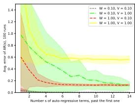
2 4 6 8 10 12 14

Number s of auto-regressive terms, past the first one 0.0

0.2 0.4 0.6 0.8 1.0 1.2 1.4

Avg. error of AR(s), 100 runs

W = 0.10, V = 0.10 W = 0.10, V = 1.00 W = 1.00, V = 0.10 W = 1.00, V = 1.00

Figure 4: The error of AR(s+ 1) as a function of s+ 1, in terms of the mean and standard deviation overN = 100 runs on Example 7, for 4 choices ofW, vof process and observation noise, respectively.

Kalman filter performs approximately as well as the bestθL.

Specifically, we have

min

L∈S T

X

t=0

`(Yt,yˆt(θL))≤min L∈S

T

X

t=0

`(Yt, ft(L)) +εT (51)

Because by constructionθL∈ D, clearly it holds that

min

φ∈D

T

X

t=0

`(Yt,yˆt(φ))≤min L∈S

T

X

t=0

`(Yt,yˆt(θL)),

and therefore combining (50) and (51) yields the statement of Theorem 6.

Experiments

To illustrate our results, we present experiments on a few well-known examples in the Supplementary Material. Out of those, we chose one to present here:

Example 7 (Adapted from (Hazan, Singh, and Zhang 2017)). Consider the system:

G= diag([0.999,0.5]), F0 = [1,1], (52)

with process noise distributed asωt ∼ N(0, w·Id2)and

observation noise νt ∼ N(0, v) for different choices of

v, w >0.

In Figure 2, we compare the prediction error for 4 meth-ods: the standard baseline last-value predictionytˆ+1 :=yt,

also known as persistence prediction, the spectral filtering of (Hazan, Singh, and Zhang 2017), Kalman filter, and AR(2). Here AR(2) is the truncation of Kalman filter, given by (13) with regression depths = 1and no remainder term. Aver-age error over 100 observation sequences generated by (52) withv = w = 0.5is shown as solid line, and its standard deviation is shown a as shaded region. Note that from some time on, spectral filtering essentially performs persistence prediction, since the inputs are zero. Further, note that both Kalman filter and AR(2) considerably improve upon the per-formance of last- value prediction.

In Figure 3, we compare the performance of AR(2) and Kalman filter under varying magnitude of noises v, w. In particular, colour indicates the ratio of the errors of Kalman filter to the errors of AR(2), wherein the errors are the av-erage prediction error over 10 trajectories of (52) for each cell of the heat-map, with each trajectory of length 50. (The formula is given in the Supplementary Material.) Consis-tent with our analysis, one can observe that increasing the variance of process noise improves the approximation of the Kalman filter by AR(2).

Finally, in Figure 4, we illustrate the decay of the remain-der term by presenting the mean (line) and standard devia-tion (shaded area) of the error as a funcdevia-tion of the regres-sion depths. There, 4 choices of the covariance matrixW

of the process noise and the variancev of the observation noise are considered within Example 7 and the error is av-eraged overN = 100runs of lengthT = 200. Of course, as expected, increasingsdecreases the error, until the error approaches that of the Kalman filter. Observe again that for a given value of the observation noise, the convergence w.r.t

sis slower forsmallerprocess noise, consistently with our theoretical observations.

Conclusions

com-peting against a class of methods, which includes Kalman filters.

We hope that our algorithms and Python code available from https://github.com/jmarecek/OnlineLDS will spur fur-ther research in forecasting and system identification.

Acknowledgments

This research received funding from the European Union Horizon 2020 Programme (Horizon2020/2014-2020) under grant agreement number 688380 (project VaVeL).

References

Anava, O.; Hazan, E.; Mannor, S.; and Shamir, O. 2013. Online learning for time series prediction. InCOLT 2013 -The 26th Annual Conference on Learning -Theory, June 12-14, 2013, Princeton University, NJ, USA.

Anderson, B., and Moore, J. 1979.Optimal Filtering. Pren-tice Hall.

Cesa-Bianchi, N., and Lugosi, G. 2006. Prediction, learn-ing, and games. Cambridge university press.

Chui, C., and Chen, G. 2017. Kalman Filtering: with Real-Time Applications. Springer International Publishing. Gardner, E. S. Exponential smoothing: The state of the art.

Journal of Forecasting4(1):1–28.

Hamilton, J. 1994.Time Series Analysis. Princeton Univer-sity Press.

Harrison, P. J. 1997. Convergence and the constant dynamic linear model.Journal of Forecasting16(5).

Hazan, E.; Singh, K.; and Zhang, C. 2017. Online learning of linear dynamical systems. InAdvances in Neural Infor-mation Processing Systems, 6686–6696.

Hazan, E. 2016. Introduction to online convex optimization.

Found. Trends Optim.

Liu, C.; Hoi, S. C. H.; Zhao, P.; and Sun, J. 2016. Online arima algorithms for time series prediction. AAAI’16. Roweis, S., and Ghahramani, Z. 1999. A unifying review of linear gaussian models. Neural Computation11(2):305– 345.

van Overschee, P., and de Moor, L. 1996. Subspace identi-fication for linear systems: theory, implementation, applica-tions. Kluwer Academic Publishers.

Venkatraman, A.; Sun, W.; Hebert, M.; Bagnell, J.; and Boots, B. 2016. Online instrumental variable regression with applications to online linear system identification. In

AAAI Conference on Artificial Intelligence, 2101–2107. West, M., and Harrison, J. 1997. Bayesian Forecasting and Dynamic Models (2nd ed.). Springer-Verlag.