The Thirty-Third AAAI Conference on Artificial Intelligence (AAAI-19)
Refining Coarse-Grained Spatial Data Using
Auxiliary Spatial Data Sets with Various Granularities
Yusuke Tanaka,
1,3Tomoharu Iwata,
2Toshiyuki Tanaka,
3Takeshi Kurashima,
1Maya Okawa,
1Hiroyuki Toda
11NTT Service Evolution Laboratories, NTT Corporation 2NTT Communication Science Laboratories, NTT Corporation
3Graduate School of Informatics, Kyoto University
{tanaka.y, iwata.tomoharu, kurashima.takeshi, okawa.maya, toda.hiroyuki}@lab.ntt.co.jp, [email protected]
Abstract
We propose a probabilistic model for refining coarse-grained spatial data by utilizing auxiliary spatial data sets. Existing methods require that the spatial granularities of the auxiliary data sets are the same as the desired granularity of target data. The proposed model can effectively make use of auxiliary data sets with various granularities by hierarchically incorpo-rating Gaussian processes. With the proposed model, a distri-bution for each auxiliary data set on the continuous space is modeled using a Gaussian process, where the representation of uncertainty considers the levels of granularity. The fine-grained target data are modeled by another Gaussian process that considers both the spatial correlation and the auxiliary data sets with their uncertainty. We integrate the Gaussian process with a spatial aggregation process that transforms the fine-grained target data into the coarse-grained target data, by which we can infer the fine-grained target Gaussian process from the coarse-grained data. Our model is designed such that the inference of model parameters based on the exact marginal likelihood is possible, in which the variables of fine-grained target and auxiliary data are analytically integrated out. Our experiments on real-world spatial data sets demon-strate the effectiveness of the proposed model.
1
Introduction
Many cities around the world are now collecting large amounts of spatial data from a wide range of sources. Gov-ernments and other organizations are releasing data on items such as poverty rate, air pollution, traffic flow, energy con-sumption and crime (Shadbolt et al. 2012; Goldstein and Dyson 2013; Barlacchi et al. 2015). Analyzing such spa-tial data is of critical importance in improving the life qual-ity of citizens in many fields such as socio-economics (Ru-pasinghaa and Goetz 2007; Smith, Mashhadi, and Capra 2014), public health (Jerrett et al. 2013), public security (Bo-gomolov et al. 2014; Wang et al. 2016) and urban plan-ning (Yuan, Zheng, and Xie 2012). For example, knowing the spatial distribution of poverty enables us to optimize al-location of resources for remedial action. Likewise, the spa-tial distribution of air pollution is useful in creating policies that can control air quality and thus protect human health.
Copyright c2019, Association for the Advancement of Artificial Intelligence (www.aaai.org). All rights reserved.
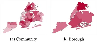
(a) Community (b) Borough
Figure 1: The distribution of poverty rates at different spatial granularities.
Naturally, information at fine spatial granularity is pferred because it allows us to identify key regions that re-quire intervention to improve city environments efficiently. As an example, Figures 1(a) and 1(b) visualize the distri-butions of poverty rates in New York City by community district and by borough, respectively; darker hues represent poorer regions. Clearly, to better understand socio-economic problems, Figure 1(a) is better than Figure 1(b). In practice, however, such information is often aggregated into coarse granularities as in Figure 1(b). It is usually thought to be too time-consuming and costly to conduct acensusover the whole population of a city, and asample surveyis conducted instead. Accordingly, the number of samples associated with each fine-grained region may not be large enough to provide a statistically significant estimate of the value associated to this region; the typical response is to aggregate samples over larger regions (Smith, Mashhadi, and Capra 2014).
geographi-cal partitions. For example, New York City has released var-ious spatial data sets portioned into boroughs, community districts, zip code, police precincts and so on.
We propose a probabilistic model for refining coarse-grained target data via the effective use of auxiliary data sets with various granularities. An important characteristic is discerning the usefulness of each auxiliary data set which depends on not only the strength of relationship with the tar-get data but also the level of spatial granularity. For exam-ple, consider the case of two auxiliary data sets that have the same strength of relationship with the target data, but differ-ent granularities. In that case, the finer-grained one is seen as more helpful for refining the coarse-grained target data.
With the proposed model, the fine-grained target data are assumed to follow a Gaussian process (GP) (Rasmussen and Williams 2006) whose mean function is modeled by a linear regression of the auxiliary data sets. This GP-based model-ing allows us to consider the spatial correlation in the tar-get data and the auxiliary data sets simultaneously. Since the target data are observed not at fine granularity but at coarse granularity, we model a spatial aggregation process to trans-form the fine-grained target data into the coarse-grained tar-get data. Furthermore, to handle auxiliary data sets with var-ious granularities, we apply GP regression to each auxiliary data set to derive a predictive distribution defined on the con-tinuous space; this conceptually corresponds to spatial inter-polation. A key idea is that it hierarchically incorporates the predictive distributions into the model; that is, it does not use point estimates. This enables us to consider uncertainty in the prediction of auxiliary data sets. The uncertainty is governed by several factors, one of which is sample den-sity, i.e., spatial granularity of the auxiliary data; the finer the granularity is, the lower the uncertainty is. Incorporating the uncertainty leads to effectively learning the usefulness of the auxiliary data with consideration of the levels of spatial granularity; this allows our model to accurately refine the coarse-grained target data. We predict the fine-grained tar-get data via a Bayesian inference procedure. The proposed model is designed such that the estimation of model param-eters based on the exact marginal likelihood is possible: By analytically integrating out the variables of fine-grained tar-get and auxiliary data, we can estimate the parameters with-out explicitly obtaining these variables. We construct the predictive distribution of the fine-grained target data by us-ing the estimated parameters.
2
Related Work
The problem of refining coarse-grained spatial data has been studied in various fields such as socio-economics (Smith and Capra 2016; Smith, Mashhadi, and Capra 2014), agricultural economics (Howitt and Reynaud 2003; Xavier et al. 2016), epidemiology (Sturrock et al. 2014) , meteorology (Wilby et al. 2004; Zorita and von Storch 1999) and geographical information system (GIS) (Boucher and Kyriakidis 2006; Goovaerts 2010). This problem is also called statistical downscaling, spatial disaggregation, and areal interpola-tion. The previous works can be categorized into two cases in terms of target data availability.
In the first case, in which a large amount of coarse- and fine-grained target data are available, we can predict the fine-grained target data by using a mapping function from coarse- to fine-grained data. The mapping function can be learnt by using various machine learning methods includ-ing linear regression models (Hessami et al. 2008), neural networks (Cannon 2011; Misra, Sarkar, and Mitra 2017) and support vector machines (Ghosh 2010). Recently, super-resolution techniques based on deep neural networks have been applied for refining coarse-grained spatial data (Vandal et al. 2017; 2018). The super-resolution techniques aim to learn a mapping function from low- to high-resolution im-ages (Dong et al. 2014). The method by (Vandal et al. 2017) is based on the analogy between gridded spatial data and images; values at grid cells are regarded as values at pixels. The large amount of fine-grained data needed for training are, however, not available in many cases (e.g., poverty sur-vey), and often only coarse-grained data are available. These methods are not applicable in such situations.
In the second case, in which only coarse-grained tar-get data are available, many regression-based methods have been proposed that use auxiliary spatial data sets to re-fine coarse-grained target data (Flaxman, Wang, and Smola 2015; Smith, Mashhadi, and Capra 2014; Wang et al. 2016; Zheng, Liu, and Hsieh 2013; Zheng et al. 2015). Regression models (linear and non-linear) are used for estimating the re-lationships between target data and auxiliary data sets. A few methods can construct the regression models under the spa-tial aggregation constraints (Murakami and Tsutsumi 2011; Park 2013). The constraints state that a value associated with a coarse-grained region is a linear average of their con-stituent values in a fine-grained partition. In order to sat-isfy the spatial aggregation constraints, the regression resid-uals at the coarse-grained regions are allocated to the fine-grained regions by using the spatial interpolation method, i.e., kriging (Stein 1999). These methods, however, assume that the auxiliary data sets have spatial granularities equiva-lent to that of fine-grained target data to be estimated. This assumption makes it difficult to utilize multiple auxiliary data sets with various granularities.
Several regression methods have been developed for estimating relationships between multi-scale spatial data sets (Miller et al. 2015; Diodato et al. 2010; Xu 2017; Xu et al. 2018). These methods predict the target data with the same granularity as that of the training data by utilizing multi-scale auxiliary data sets. They do not, however, con-sider the spatial aggregation constraint, which is a critical factor in refining the coarse-scale target data.
There have been several hierarchical Bayesian models to predict fine-grained target data using fine-grained aux-iliary data sets. Although they introduce a fully Bayesian inference (Taylor, Andrade-Pacheco, and Sturrock 2018; Wilson and Wakefield 2018; Keil et al. 2013) or a variational inference (Law et al. 2018) for model parameters, the uncer-tainty in the prediction of auxiliary data sets is ignored: They cannot discern the usefulness of each auxiliary data set con-sidering their levels of spatial granularity.
granu-Table 1: Notation.
Symbol Description
S set of indices of auxiliary spatial data sets
s index of auxiliary spatial data set,s∈ S X total region of a city
x location point represented by
latitude and longitude coordinates,x∈ X Pcoar
coarse-grained partition ofXof target data
i region in the coarse-grained partition of target data,i∈ Pcoar
Pfine
fine-grained partition ofXof target data
j region in the fine-grained partition of target data,j∈ Pfine
Ps partition ofXofsth auxiliary data set
p region in the partition ofsth auxiliary data set,p∈ Ps
ai value associated with regioniin coarse-grained
target data,ai∈R
zj value associated with regionjin fine-grained
target data,zj∈R
ys,p value associated with regionpinsth auxiliary
data set,ys,p∈R
larities by hierarchically incorporating Gaussian processes. This hierarchical modeling allows us to effectively learn the usefulness of each auxiliary data set considering the lev-els of spatial granularity. Our model also considers the spa-tial aggregation constraints by integrating the Gaussian pro-cesses with a spatial aggregation process to transform the fine-grained target data into the coarse-grained target data.
3
Problem Formulation
In this section, we describe the spatial data this study fo-cuses on, and define our problem of refining coarse-grained spatial data by using, for the same region, auxiliary spatial data sets with various granularities. Assume that we have a target spatial data set with coarse granularity, and we would like to obtain a fine-grained version. LetSbe the collection of indices of auxiliary data sets. The notations used in this paper are listed in Table 1.
Partition:LetXbe a total region of a city, andx∈ X be a location point represented by its coordinates (e.g., latitude and longitude). PartitionP ofX is a collection of disjoint subsets, called regions, of X, whose union is equal toX. Let|P|denote the number of regions inP. We can consider several partitions ofX as follows. LetPcoarbe the coarse-grained partition, i.e., that of the coarse-coarse-grained target data. LetPfinebe the grained partition, of the desired fine-grained target data. Fors∈ S, letPsbe the partition of the
sth auxiliary data set.
Spatial data:Leta = (a1, . . . , a|Pcoar|)> be a|Pcoar |-dimensional vector consisting of the coarse-grained target values, whereai ∈ R is the value associated with region i ∈ Pcoar. Fors ∈ S, lety
s = (ys,1, . . . , ys,|Ps|)> be a
|Ps|-dimensional vector consisting of thesth auxiliary data
values, whereys,p ∈ Ris the value associated with region p∈ Psof thesth auxiliary data set.
Problem: Suppose that we have coarse-grained target dataawhose partition isPcoar, auxiliary data sets with the respective partitions {(Ps,ys) | s ∈ S}, and the desired
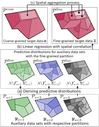
Figure 2: Generative process of coarse-grained target data given three auxiliary data sets.
fine-grained partition Pfine, we wish to estimate a|Pfine |-dimensional vectorz = (z1, . . . , z|Pfine|)>consisting of the fine-grained target values, wherezj ∈Ris the value
associ-ated with regionj ∈ Pfine. Here, the valuesa
i,ys,pandzj
are assumed to be intensive quantities such as ratios; that is, they are independent of the area scale of the respective re-gions. When the values are extensive quantities such as pop-ulation, they can be transformed into intensive quantities by dividing them with the areas of regions.
4
Proposed Model
We propose a probabilistic model that allows auxiliary spa-tial data sets with various granularities to be used in refining coarse-grained spatial data. Our model is based on Gaus-sian process (GP) (Rasmussen and Williams 2006), which is a flexible non-parametric model for non-linear functions in a continuous domain. We model the generative process for coarse-grained target data a, given the auxiliary data sets with known partitions {(Ps,ys) | s ∈ S}, coarse-grained
partition Pcoar, and fine-grained partition Pfine. In other words, we model the conditional probabilityp(a| {ys}s∈S)
instead of the joint probability ofaand{ys}s∈S. It enables
us to adopt two-step inference approach described in Sec-tion 5, which is advantageous in the computaSec-tional cost for learning model parameters.
con-tinuous predictive distributions of the auxiliary data sets; (c) generating the coarse-grained target dataaby spatially ag-gregating the constituent values in a fine-grained partition.
In our problem, each value is associated with a region in a partition rather than a single location point inX; this pre-vents us from directly applying GP. We thus associate each region in a partition with its centroid, and regard each value as being associated with the centroid of that region. This as-sumption, while significantly simplifying computations in-volved, might worsen the fit of the GP to the data set, which however is appropriately taken into account in the following steps as increased uncertainty of the GPs for both the respec-tive auxiliary data sets (described in (5)) and the target data (described in (6)). Fors ∈ S, letXs = (xs,1, . . . ,xs,|Ps|)
be the set of the centroids in partitionPs, wherexs,pis the
centroid of regionp∈ Ps. Similarly, for fine-grained
parti-tionPfine, letXfine = (x
1, . . . ,x|Pfine|)be the set of cen-troids in Pfine. Thus, our problem is now reformulated as estimatingz= (z1, . . . , z|Pfine|)>, wherezj ∈Ris a target
value at the centroid of regionj∈ Pfine, as indicated by the auxiliary spatial data sets{(Xs,ys)|s∈ S}.
(a) Deriving predictive distributions of auxiliary spa-tial data sets:In order to handle auxiliary spatial data sets with various granularities, we use GP regression to derive a posterior Gaussian process for a latent continuous random function onX; this conceptually corresponds to spatial inter-polation of each auxiliary spatial data set. We then evaluate the predictive distribution on the basis of the posterior Gaus-sian process. Letfs(x)be a noise-free latent function for the
sth auxiliary data set at locationx. We assume thatfs(x)
follows a Gaussian process, fs(x) ∼ GP(0, ks(x,x0)),
with mean zero and a covariance functionks(x,x0). Though
our model does not depend on any particular choice of the covariance function, for simplicity we consider the well-known covariance function, i.e., squared-exponential ker-nel, which is widely used for measuring the similarity be-tween function values in spatial coordinates (Rasmussen and Williams 2006). The squared-exponential kernel is defined as
ks(x,x0) =α2sexp
− 1
2γ2
s
kx−x0k2
, (1) where γs is the scale parameter, α2s is a signal variance
that controls the magnitude of the covariance, and k · k is the Euclidean norm. We assume that the sth auxil-iary data ys is generated with an additive Gaussian noise with noise varianceσ2s. Definingfs∗(xp)as the prediction
of the sth auxiliary data set for the centroid xp of the
fine-grained partition, the predictive distribution of f∗s = (fs∗(x1), . . . , fs∗(x|Pfine|))>is as follows:
p(f∗s) =N(f∗s|f¯∗s,Σ∗s), (2) wheref¯∗s =K>s∗(Ks+σ2
sI)−1ysis the predictive means,
andΣ∗s=Ks∗∗−K>s∗(Ks+σ2sI)−1Ks∗is the covariance
matrix, whose diagonal elements represent the uncertainties in the prediction at the test pointsXfine. Incorporation of the predictive distributions (2) is expected to allow the use-fulness of auxiliary data to be effectively learnt as it allows consideration of the uncertainty in the prediction. Details are
given in (7) in Section 5. Here,Ksis a|Ps| × |Ps|
covari-ance matrix whose entries are covaricovari-ances between training pointsXs.Ks∗is a|Ps| × |Pfine|covariance matrix whose
entries are covariances between training pointsXsand test pointsXfine.K
s∗∗ is a|Pfine| × |Pfine|covariance matrix
whose entries are covariances between test pointsXfine. (b) Generative process of fine-grained target data:We model a generative process for the fine-grained target dataz. Letz(x)be a noise-free latent function for the fine-grained target data at location x. We assume that z(x) follows a Gaussian process,z(x)∼ GP(m(x), k(x,x0)), with mean functionm(x) =P
s∈Swsfs(x) +w0, wherews∈Rand w0 ∈ Rare the regression coefficient of thesth auxiliary
data set and the bias parameter, respectively. The covariance functionk(x,x0)is a squared-exponential kernel with the scale parameterγand signal varianceα2. Given the predic-tive values for the auxiliary data sets from (2), the condi-tional distribution ofzat the centroidsXfineis given by
p(z|F∗) =N(z|F∗w,K), (3) wherew= (w0, . . . , w|S|)>andKis a|Pfine| × |Pfine|
co-variance matrix defined byk(x,x0). Here, we let|S|be the number of auxiliary data sets. We define the augmented ma-trix as the|Pfine| ×(|S|+ 1)matrixF∗= (f∗
1, . . . ,f
∗ |S|,1),
in which1is a column vector of 1’s. This GP-based model-ing enables us to consider the spatial correlation in the target data and the auxiliary data sets simultaneously.
(c) Generative process of coarse-grained target data: We design a spatial aggregation process to transform the fine-grained target datazinto the coarse-grained target data
a, in order to encourage consistency betweenz , which is to be estimated, and the available coarse-grained target data
a. In the spatial aggregation process, a value associated with one region in the coarse-grained partition is obtained by ag-gregating the values in the fine-grained regions contained in the coarse-grained region (see the upper part of Figure 2). Then,a is generated from the following conditional distri-bution givenz,
p(a|z) =N(a|Hz, σ2I), (4) whereσ2is the noise variance for the coarse-grained target data, andHis a|Pcoar| × |Pfine|aggregation matrix, whose entries are nonnegative weighting coefficients; the row sum ofHshould equal 1. We set the coefficients in accordance with the property of the target data. For example, in cases where target data are incidences of disease, then the(i, j) -entryH(i, j)ofHwould be proportional to the population in the intersection of the coarse-grained regioniand the fine-grained region j. In the following, for simplicity, we con-sider a simple aggregation matrix, in which entry H(i, j)
is1/|Pfine
i | if the fine-grained regionj is contained in the
coarse-grained regioni, and zero otherwise. Here,Pfine
i is a
subset ofPfine, all the elements of which are contained in the coarse-grained regioni∈ Pcoar.
5
Inference
Algorithm 1: Bayesian inference procedure of the fine-grained target dataz
Input :a,{(Xs,ys)|s∈ S},X
fine
,H Output:Predictive distribution ofz
1: Initialize model parameters,{αs|s∈ S},{γs|s∈ S},
{σs|s∈ S},w,α,γ,σ
2: /* first inference step */ 3: fors∈ Sdo
4: Estimateαs, γs, σsby maximizing the logarithm of (5)
5: end for
6: /* second inference step */
7: Estimatew, α, γ, σby maximizing the logarithm of (6) 8: Construct predictive distribution ofzby (8) using the
estimated model parameters
of fine-grained partition Xfine and the aggregation matrix
H, we aim to predict the fine-grained target data z via a Bayesian inference procedure. In order to calculate the pre-dictive distribution ofz, we need to estimate the model pa-rameters. The problem of estimating the model parameters can be divided into two steps: 1) Estimate hyperparameters αs, γs, σsfor each auxiliary data set and 2) estimate
regres-sion coefficientw and hyperparametersα, γ, σ for the tar-get data. Although one could also opt for estimating all the model parameters simultaneously (i.e., one-step inference), it will increase the computational cost of inference drasti-cally; we adopt the efficient two-step inference as described in the following paragraphs. We finally construct the pre-dictive distribution ofz by using the estimated parameters. Details of the inference procedure are shown in Algorithm 1. The first inference step:Given thesth auxiliary spatial data set with centroids(Xs,ys), the marginal likelihood of ysis given by
p(ys|αs, γs, σs) =N(ys|0,Ks+σ
2
sI). (5)
The hyperparametersαs, γs, σs are estimated by
maximiz-ing the logarithm of (5). We solve the optimization prob-lem through the use of the BFGS method (Liu and Nocedal 1989). By solving the optimization problem for each aux-iliary data set independently, we obtain the set of the esti-mated hyperparameters for all auxiliary data sets. The pre-dictive distribution of f∗s corresponding to (2) is obtained using the estimated hyperparameters.
The second inference step:Given the coarse-grained tar-get dataaand the centroids of fine-grained partitionXfine, the marginal likelihood ofais given by
p(a|w, α, γ, σ) = Z Z
p(a|z)p(z|F∗)Y
s∈S
p(f∗s)dF
∗
dz
= Z Z
N a|Hz, σ2I
N(z|F∗w,K)
×Y
s∈S
N f∗s|f¯
∗
s,Σ
∗
s
dF∗dz
=N a|HF¯∗w,Λ
, (6)
whereF¯∗ = ( ¯f∗1, . . . ,f¯|S|∗ ,1)is a|Pfine| ×(|S|+ 1) ma-trix, and we analytically integrate out the latent variables
F∗ and z with the help of the conjugacy of the distribu-tions (2), (3), and (4). Λis a|Pcoar| × |Pcoar|covariance matrix represented by Λ = σ2I+HΩH>, where Ω =
K+P
s∈Sws2Σ ∗
s. The(i, i0)-entryΛ(i, i0)ofΛis shown
in (7). Here,δ•,•in (7) represents Kronecker delta;δA,B= 1
ifA = B, andδA,B = 0otherwise. The residual variance
term in (7) represents the residual variance in the regression ofz(xj). This term contains the uncertainty in the prediction
offs(xj), i.e.,Σ∗s(j, j), which is weighted byws2. The
spa-tial correlation term in (7) represents the strength of spaspa-tial correlation between z(xj)andz(xj0). This term contains the covariance betweenfs(xj)andfs(xj0), i.e.,Σ∗s(j, j0), which is weighted byw2
s. On the basis of the marginal
like-lihood (6) with this covariance matrix Λ, our model can effectively learn the regression coefficient w while taking into consideration the prediction uncertainties and the spatial correlations from the auxiliary data sets with various gran-ularities, simultaneously. The parameterw and the hyper-parametersα,γ,σare estimated by maximizing the loga-rithm of (6). We solve the optimization problem by using the BFGS method (Liu and Nocedal 1989). The derivatives of the logarithm of (6) with respect tows,α,γ,σ are
de-scribed in Appendix A.
Predictive distribution of fine-grained target data: Us-ing the estimated model parameters, the predictive distribu-tion of the fine-grained target datazis given by
p(z∗) =N(z∗|z¯∗,cov(z∗)), (8)
where¯z∗ = ¯F∗w+ΩH>Λ−1(a−F¯∗w)is the predictive means, and where cov(z∗) = Ω−ΩH>Λ−1HΩ is the covariance matrix. We can obtain the refinement results, i.e., the estimated fine-grained target data, by using the predictive means¯z∗. By analyzing the covariance matrixcov(z∗), we
can also evaluate the confidence of the refinement results.
Λ(i, i0) =σ2δi,i0+ 1 |Pfine
i ||P
fine
i0 |
× X
j∈Pfine
i
X
j0∈Pfine
i0
"
δj,j0 α2+ X
s∈S
w2sΣ
∗
s(j, j
0
) !
| {z }
residual variance term
+(1−δj,j0) α2exp
− 1
2γ2kxj−xj0k 2
+X
s∈S
ws2Σ
∗
s(j, j
0
) !
| {z }
spatial correlation term
#
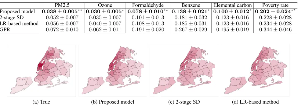
Table 2: MAPELand standard errors for the predictions of the fine-grained target data.
PM2.5 Ozone Formaldehyde Benzene Elemental carbon Poverty rate Proposed model 0.038±0.005?? 0.030±0.005? 0.078±0.010?? 0.138±0.021? 0.100±0.012? 0.202±0.024??
2-stage SD 0.052±0.007 0.035±0.007 0.101±0.013 0.181±0.032 0.123±0.016 0.228±0.028
LR-based method 0.056±0.007 0.040±0.007 0.108±0.013 0.185±0.031 0.123±0.016 0.234±0.028
GPR 0.072±0.010 0.062±0.011 0.191±0.020 0.267±0.029 0.195±0.019 0.344±0.046
(a) True (b) Proposed model (c) 2-stage SD (d) LR-based method
Figure 3: Comparison of the predicted fine-grained target data for PM2.5 data set.
6
Experiments
Data description:We evaluated the proposed model using real-world spatial data sets from NYC Open Data1. There are 44 data sets that contain a variety of categories such as social indicators, land use, air quality and taxi traffic. Each data set is associated with one of six geographical parti-tions, i.e., school district (32), UHF42 (42), community dis-trict (59), police precinct (77), zip code (186) and taxi zone (249), where each number in parenthesis denotes the num-ber of regions in the corresponding partition. In our exper-iments, we try to refine the poverty rate data set and the five air pollution data sets (i.e., PM2.5, ozone, formalde-hyde, benzene, elemental carbon). The experimental setting is as follows: 1) Given the poverty rate data set with the bor-ough partition (|Pcoar|= 5), we would like to refine the data into the community district partition (|Pfine| = 59), and 2) given each air pollution data set with the borough partition (|Pcoar|= 5), we aim to refine the data into the UHF42 par-tition (|Pfine| = 42). Appendix B details the data sets and the experimental settings.
Baselines:The existing methods can be applied to aux-iliary data sets with various granularities if pre-processing is applied, i.e., spatial interpolation, so that the granularities of the auxiliary data sets match with that of the fine-grained target data. Accordingly, we first performed spatial interpo-lation of each auxiliary data setysby using GP regression;
we then obtained the predictive valuesf¯∗s at the centroids
Xfineof the target fine-grained partition so that the spatial granularities of all auxiliary data sets equaled that of the fine-grained target data. We compared the proposed model with three baselines: GP regression (GPR) (Rasmussen and Williams 2006), Linear regression-based method (LR-based method) (Smith, Mashhadi, and Capra 2014) and Two-stage statistical downscaling method (2-stage SD) (Park 2013). Here, GPR is a simple spatial interpolation, namely, it
pre-1
https://opendata.cityofnewyork.us
Table 3: Top-10 relevant auxiliary data as estimated by our model and 2-stage SD for PM2.5 data set.
Proposed model 2-stage SD
Auxiliary data ws Auxiliary data ws
1. Fire incident (Zip code) 0.173 1-2 fam. bldg (Comm.) -0.088 2. Taxi dropoff (Taxi zone) 0.139 Hospital (Comm.) 0.069 3. 311 call (Zip code) 0.135 Public school (Comm.) 0.069 4. Public telephone (Zip code) 0.114 Lots of vacant (Comm.) -0.067 5. Natural gas (Zip code) 0.109 Crime (Police precinct) 0.064 6. Mean commute (Comm.) -0.109 Unemployment (Comm.) 0.063 7. 1-2 fam. bldg (Comm.) -0.089 Pct. served parks (Comm.) 0.062 8. Pct. served park (Comm.) 0.075 Library (Comm.) 0.061 9. GHG emission (Zip code) 0.068 Fire incident (Zip code) 0.059 10. Population (Comm.) 0.062 Park (Comm.) 0.058
dicts the fine-grained target datazby using only the coarse-grained target dataa. Details of these baselines are given in Appendix C.
Fine-grained target data prediction:We evaluated our model in terms of its performance in predicting fine-grained target data z. The evaluation metric is the mean absolute percentage error (MAPE) in fine-grained target values:L=
1
|Pfine| P
j∈Pfine
ztruej −z∗
j ztrue
j
, wherez
true
j is the true value
(a) True (b) Proposed model (c) 2-stage SD (d) LR-based method
Figure 4: Comparison of the predicted fine-grained target data for poverty rate data set.
(a) Fire incidents (b) Taxi dropoff
Figure 5: Top-2 auxiliary data sets ranked by the proposed model for PM2.5 data set.
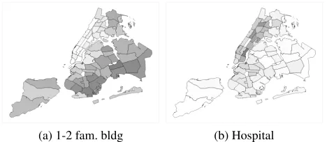
(a) 1-2 fam. bldg (b) Hospital
Figure 6: Top-2 auxiliary data sets ranked by the 2-stage SD for PM2.5 data set.
Figures 3 and 4 visualize the predicted fine-grained target datazfor the PM2.5 data set and for the poverty rate data set, respectively. We illustrate the true fine-grained data on the left in Figures 3 and 4, and the predictions made by the proposed model, 2-stage SD and LR-based method on the right. Here, the predictive values of each method were nor-malized to the range[0,1], and darker hues represent regions with higher values. As shown in these figures, our model re-fined the coarse-grained data more precisely than the other methods. In particular, in both data sets, our model achieved significant improvement in the north part of the map (i.e., Manhattan). Such visualization results are useful for finding key regions, e.g., the poorest regions of a city.
Evaluation of auxiliary spatial data sets:Table 3 shows the top ten relevant auxiliary data sets as determined by our model and 2-stage SD for the PM2.5 data set. These auxil-iary data sets are arranged in descending order of the abso-lute values of the estimated regression coefficient w, each of which is listed in the “ws” columns of Table 3. By
com-paring the sorted list of the auxiliary data sets created by the proposed model with that yielded by 2-stage SD, we can confirm that the proposed model assigned relatively large regression coefficients to the auxiliary data sets with finer-grained partitions (i.e., Zip code and Taxi zone).
Figures 5 and 6 visualize the top two relevant auxiliary data sets as estimated by our model and 2-stage SD for the PM2.5 data set, respectively. Comparing these visualizations with that of the true target data in Figure 3(a) shows that our model emphasized the most useful auxiliary data sets, i.e., those that are both strongly related with the target data and have fine granularities; 2-stage SD evaluated the usefulness of auxiliary data sets only in terms of the strength of rela-tionships between the target data and the auxiliary data sets in the coarse-grained partition.
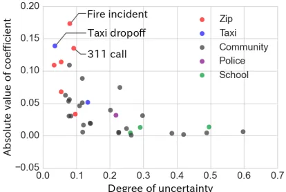
Figure 7 shows the relation between the regression co-efficient and the uncertainty in the prediction of auxiliary data sets estimated by the proposed model for the PM2.5 data set. In this figure, each auxiliary data set is depicted by a dot whose color indicates its partition. The horizon-tal axis shows the averages of the variances in the pre-dicted values of each auxiliary data set; for the sth aux-iliary data set, the average of variances was calculated by
(1/|Pfine|)P
j∈PfineΣ∗s(j, j), which is the degree of
uncer-tainty in predicting the sth auxiliary data set; the vertical axis shows the absolute values of the estimated coefficients. As shown, the absolute coefficient values estimated by our model were likely to be higher for the auxiliary data sets that had lower degrees of uncertainty. These results indicate that our model can effectively learn the usefulness of each auxil-iary data set by considering the uncertainty in the prediction of auxiliary data sets. Consequently, the proposed model can precisely refine the coarse-grained target data by effectively utilizing auxiliary data sets with various granularities.
7
Conclusion
Us-Figure 7: Relation between the coefficients and the uncer-tainties for PM2.5 data set.
ing multiple real-world spatial data sets in New York City, we confirmed that our model can predict the fine-grained target data more precisely compared with the baselines.
Our future work is to consider shapes of regions as in the previous study (Rathbun 1998): The assumption of using the centroid of each region allows for GP-based formulations and significantly simplifying computations involved; mean-while, it might worsen the fit of the GP to the exotic shaped regions (e.g., extremely elongated). Another future work is to incorporate fully Bayesian treatment for model parame-ters. It can be expected to provide the better results.
A
Derivatives of model parameters
The log-marginal likelihood ofais given bylogp(a|w, α, γ, σ) =−1 2(a−H
¯
F∗w)>Λ−1(a−HF¯∗w)
−1
2log (det(Λ))− |Pcoar|
2 log 2π. (9)
We describe the first derivatives of (9) with respect tows,α,
γ,σ, which is required for estimating the parameter based on the BFGS method. The derivative of (9) with respect to wsis given by
∂ ∂ws
logp(a|w, α, γ, σ)
=∂(a−H ¯
F∗w) ∂ws
p+1
2tr
(pp>−Λ−1)∂Λ ∂ws
, (10)
where p = Λ−1(a −HF¯∗w) and ∂Λ/∂ws is a matrix
of elementwise derivatives. The derivative of the element
Λ(i, i0)(7) is obtained by ∂Λ(i, i0)
∂ws
= 1
|Pfine
i ||Pifine0 | X
j∈Pfine
i
X
j0∈Pfine
i0
2wsΣ∗s(j, j 0).
(11) Denotingθ∈ {α, γ, σ}, the derivative of (9) with respect to θis given by
∂
∂θlogp(a|w, α, γ, σ) = 1 2tr
(pp>−Λ−1)∂Λ ∂θ
. (12)
The matrix of elementwise derivatives∂Λ/∂θis trivial. The derivative of the element Λ(i, i0)(7) with respect to each hyperparameter is as follows:
∂Λ(i, i0) ∂α
= 1
|Pfine
i ||Pifine0 | X
j∈Pfine
i
X
j0∈Pfine
i0
2αexp
− 1
2γ2kxj−xj0k 2
,
(13)
∂Λ(i, i0)
∂γ =
1 |Pfine
i ||Pifine0 | X
j∈Pfine
i
X
j0∈Pfine
i0 α2
1
γ3kxj−xj0k 2
×exp
− 1
2γ2kxj−xj0k 2
, (14)
∂Λ(i, i0)
∂σ = 2σδi,i0. (15)
B
Description of real-world spatial data sets
We used the real-world spatial data sets from NYC Open Data 2. for evaluating the proposed model. The data sets were collected and released for improving the urban envi-ronment in New York City, and contain a variety of cate-gories such as social indicators, land use, air quality and taxi traffic. Details of the data sets are listed in Table 4. There are multiple data sets in each category, with the total number of data sets being 44. Each data set is associated with one of six geographical partitions, i.e., school district, UHF42, community district, police precinct, zip code and taxi zone. These partitions have various spatial granularities; the num-ber of regions in each partition is shown in Table 4. These data sets are gathered once a year using the time ranges shown in Table 4; the values of data are divided by the num-ber of observation times. When the values of data are exten-sive quantities (i.e., proportional to the scale of areas, e.g., population), the values are divided by the areas of respective regions; the resulting values are intensive quantities (i.e., in-dependent of area scale, e.g., population density).In our experiments, we try to refine the poverty rate data set in the social indicator category and the five air pollution data sets in the air quality category. The poverty rate data set contains the values of poverty rates associated with each re-gion in the community district partition as visualized in Fig-ure 1(a). The air pollution data sets contain the average con-centrations of pollutants (i.e., PM2.5, ozone, formaldehyde, benzene, elemental carbon) associated with each region in the UHF42 partition. In order to evaluate the performance in refining coarse-grained data, we used the data that were aggregated into a coarser-grained partition, i.e., borough par-tition, via spatial averaging, where the borough partition has five regions as illustrated in Figure 1(b). The experimental setting is as follows: 1) Given the poverty rate data set with borough partition (|Pcoar|= 5), we would like to refine the data into the community district partition (|Pfine|= 59), and 2) given each air pollution data set with the borough parti-tion (|Pcoar|= 5), we aim to refine the data into the UHF42
Table 4: Spatial data sets.
Category/Name #data sets Partition #regions Time range Description
Education 3 School district 32 2010 Class size, ratio of #pupils to #teachers, SAT score Air quality 8 UHF42 42 2009–2010 Average concentration of pollutants
Social indicator 13 Community district 59 2009–2013 Poverty rate, population, mean commute time, etc. Land use 11 Community district 59 2009–2013 Area percentage for commercial office, parking, etc. Crime 1 Police precinct 77 2010–2016 Number of crimes
Incident 2 Zip code 186 2010–2016 #311 calls, #fire incidents
Telecommunication 2 Zip code 186 2016 #public telephones, #free Wi-Fi hotspots Consumption 2 Zip code 186 2010–2014 GHG emission, natural gas consumption Taxi traffic 2 Taxi zone 249 2014–2016 #taxi pick-up and drop-off events
partition (|Pfine| = 42). In the setting for the poverty rate data set, we used all data sets other than the target data as auxiliary data sets, so the number of auxiliary data sets|S| was 43. In the setting for the air pollution data sets, we used all data sets not contained in the air quality category, so|S| was 36.
C
Baselines description
For GPR, we predict the fine-grained target data z based only on the coarse-grained target data a. For LR-based method and 2-stage SD, given the coarse-grained target data
aand the predictive values of all auxiliary data setsF¯∗, we predict the fine-grained target dataz. Details of these base-lines are given below.
Gaussian process regression (GPR): We compared our proposed model with a simple spatial interpolation (i.e., GPR) of the coarse-grained spatial dataa. This baseline as-sumes that the target data are explained by only the spatial correlation. Givenaand the set of centroids of the coarse-grained partitionPcoar, we predicted the fine-grained target data z by using the predictive distribution. Note that this baseline does not use the auxiliary spatial data sets.
Linear regression-based method (LR-based method): We used a linear regression-based method that has been applied in various studies (Bogomolov et al. 2014; Smith, Mashhadi, and Capra 2014). The linear regression model is used for estimating the relationships between the coarse-grained target data and the auxiliary data sets. The procedure in the training phase is as follows: 1) aggregate all auxil-iary data sets into the coarse-grained partition of target data via spatial averaging; 2) estimate the regression coefficients
wof the respective auxiliary data sets by using the coarse-grained target data and the auxiliary data sets aggregated via spatial averaging. In the prediction phase, generate unknown valueszfor the target fine-grained partition by applying the estimated relationships to the predictive values of auxiliary data setsF¯∗as follows:z= ¯F∗wˆ, wherewˆ is the estimated regression coefficient.
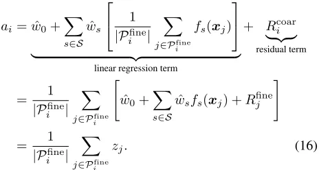
Two-stage statistical downscaling method (2-stage SD): We used the statistical downscaling method proposed in (Park 2013). This method assumes that coarse-grained tar-get dataacan be decomposed into linear regression terms and residual terms. The downscaling procedure is divided into two stages. In the first stage, we obtain the regression coefficientsw in a manner similar to the training phase of
the LR-based method. In the second stage, given the esti-mated coefficientwˆ, the fine-grained target dataz are esti-mated to be those that satisfy the following relation:
ai = ˆw0+
X
s∈S
ˆ ws
1
|Pfine
i |
X
j∈Pfine
i
fs(xj)
| {z }
linear regression term
+ Rcoari | {z } residual term
= 1
|Pfine
i |
X
j∈Pfine
i
"
ˆ w0+
X
s∈S
ˆ
wsfs(xj) +Rfinej
#
= 1
|Pfine
i |
X
j∈Pfine
i
zj. (16)
This relation expresses the spatial aggregation constraint, i.e., the assumption that value ai associated with
coarse-grained regioniis the linear average of the constituent val-ues in the fine-grained partition. Here, Rcoar
i andRfinej are
the residuals in the coarse-grained and fine-grained parti-tions, respectively. To obtain the fine-grained target dataz, the residual valueRfinej in the fine-grained partition must be determined. Since the linear regression terms have already been fixed in the first stage, Rcoari is obtained from (16); the residuals in the fine-grained partition are predicted by applying the spatial interpolation method, i.e., simple krig-ing (Kyriakidis 2004), to the residualsRcoar
i in the
coarse-grained partition.
References
Barlacchi, G.; Nadai, M. D.; Larcher, R.; Casella, A.; Chitic, C.; and G. Torrisi et al., j. 2015. A multi-source dataset of urban life in the city of Milan and the province of Trentino.Scientific Data2. Bogomolov, A.; Lepri, B.; Staiano, J.; Oliver, N.; Pianesi, F.; and Pentland, A. 2014. Once upon a crime: Towards crime prediction from demographics and mobile data. InICMI, 427–434.
Boucher, A., and Kyriakidis, P. C. 2006. Super-resolution land cover mapping with indicator geostatistics.Remote Sensing of En-vironment104:264–282.
Cannon, A. J. 2011. Quantile regression neural networks: Imple-mentation in R and application to precipitation downscaling. Com-puters & Geosciences37(9):1277–1284.
Dong, C.; Loy, C. C.; He, K.; and Tang, X. 2014. Learning a deep convolutional network for image super-resolution. InECCV, 184–199.
Flaxman, S. R.; Wang, Y. X.; and Smola, A. J. 2015. Who sup-ported Obama in 2012?: Ecological inference through distribution regression. InKDD, 289–298.
Ghosh, S. 2010. SVM-PGSL coupled approach for statistical downscaling to predict rainfall from GCM output.Journal of Geo-physical Research: Atmospheres115(D22).
Goldstein, B., and Dyson, L. 2013. Beyond Transparency: Open Data and the Future of Civic Innovation. Code for America Press. Goovaerts, P. 2010. Combining areal and point data in geostatisti-cal interpolation: Applications to soil science and medigeostatisti-cal geogra-phy.Mathematical Geosciences42(5):535–554.
Hessami, M.; Gachon, P.; Ouarda, T. B.; and St-Hilair, A. 2008. Automated regression-based statistical downscaling tool. Environ-mental Modeling & Software23(6):813–834.
Howitt, R., and Reynaud, A. 2003. Spatial disaggregation of agri-cultural production data using maximum entropy. European Re-view of Agricultural Economics30(2):359–387.
Jerrett, M.; Burnett, R. T.; Beckerman, B. S.; Turner, M. C.; Krewski, D.; Thurston, G.; and et al. 2013. Spatial analysis of air pollution and mortality in California.American Journal of Res-piratory and Critical Care Medicine188(5):593–599.
Keil, P.; Belmaker, J.; Wilson, A. M.; Unitt, P.; and Jetz, W. 2013. Downscaling of species distribution models: a hierarchical ap-proach.Methods in Ecology and Evolution4(1):82–94.
Kyriakidis, P. C. 2004. A geostatistical framework for area-to-point spatial interpolation.Geographical Analysis36(3):259–289. Law, H. C. L.; Sejdinovic, D.; Cameron, E.; Lucas, T. C. D.; Flax-man, S.; Battle, K.; and Fukumizu, K. 2018. Variational learning on aggregate outputs with Gaussian processes. InNeurIPS, 6084– 6094.
Liu, D. C., and Nocedal, J. 1989. On the limited memory BFGS method for large scale optimization. Mathematical programming
45(1–3):503–528.
Miller, B. A.; Koszinski, S.; Wehrhan, M.; and Sommer, M. 2015. Impact of multi-scale predictor selection for modeling soil proper-ties.Geoderma239–240:97–106.
Misra, S.; Sarkar, S.; and Mitra, P. 2017. Statistical downscal-ing of precipitation usdownscal-ing long short-term memory recurrent neural networks.Theor. Appl. Climatol.
Murakami, D., and Tsutsumi, M. 2011. A new areal interpola-tion technique based on spatial econometrics.Procedia-Social and Behavioral Sciences21:230–239.
Park, N. W. 2013. Spatial downscaling of TRMM precipitation us-ing geostatistics and fine scale environmental variables. Advances in Meteorology2013.
Rasmussen, C. E., and Williams, C. K. I. 2006.Gaussian Processes for Machine Learning. MIT Press.
Rathbun, S. L. 1998. Spatial modelling in irregularly shaped re-gions: Kriging estuaries.Environmetrics9:109–129.
Rupasinghaa, A., and Goetz, S. J. 2007. Social and political forces as determinants of poverty: A spatial analysis. The Journal of Socio-Economics36(4):650–671.
Shadbolt, N.; O’Hara, K.; Berners-Lee, T.; Gibbins, N.; Glaser, H.; Wendy, H.; and Schraefel, M. C. 2012. Linked open gov-ernment data: Lessons from data.gov.uk.IEEE Intelligent Systems
27(3):16–24.
Smith, C. C., and Capra, L. 2016. Beyond the baseline: Establish-ing the value in mobile phone based poverty estimates. InWWW, 425–434.
Smith, C. C.; Mashhadi, A.; and Capra, L. 2014. Poverty on the cheap: Estimating poverty maps using aggregated mobile commu-nication networks. InCHI, 511–520.
Stein, M. L. 1999.Interpolation of Spatial Data: Some Theory for Kriging. Springer.
Sturrock, H. J. W.; Cohen, J. M.; Keil, P.; Tatem, A. J.; Menach, A. L.; Ntshalintshali, N. E.; Hsiang, M. S.; and Gosling, R. D. 2014. Fine-scale malaria risk mapping from routine aggregated case data.Malaria Journal13:421.
Taylor, B. M.; Andrade-Pacheco, R.; and Sturrock, H. J. W. 2018. Continuous inference for aggregated point process data.Journal of the Royal Statistical Society: Series A (Statistics in Society)12347. Vandal, T.; Kodra, E.; Ganguly, S.; Michaelis, A.; Nemani, R.; and Ganguly, A. R. 2017. DeepSD: Generating high resolution climate change projections through single image super-resolution. InKDD, 1663–1672.
Vandal, T.; Kodra, E.; Ganguly, S.; Michaelis, A.; Nemani, R.; and Ganguly, A. R. 2018. Generating high resolution climate change projections through single image super-resolution: An abridged version. InIJCAI, 5389–5393.
Wang, H.; Kifer, D.; Graif, C.; and Li, Z. 2016. Crime rate infer-ence with big data. InKDD, 635–644.
Wilby, R. L.; Zorita, S. P.; Timbal, E.; Whetton, B.; and Mearns, L. O. 2004. Guidelines for Use of Climate Scenarios Developed from Statistical Downscaling Methods.
Wilson, K., and Wakefield, J. 2018. Pointless spatial modeling.
Biostatistics.
Wotling, G.; Bouvier, C.; Danloux, J.; and Fritsch, J. M. 2000. Re-gionalization of extreme precipitation distribution using the prin-cipal components of the topographical environment. Journal of Hydrology233(1-4):86–101.
Xavier, A.; Freitas, M. B. C.; Rosj´ario, M. D. S.; and Fragoso, R. 2016. Disaggregating statistical data at the field level: An entropy approach.Spatial Statistics23:91–103.
Xu, J.; Liu, X.; Wilson, T.; Tan, P. N.; Hatami, P.; and Luo, L. 2018. Muscat: Multi-scale spatio-temporal learning with application to climate modeling. InIJCAI, 2912–2918.
Xu, J. 2017. Multi-task learning and its application to geospatio-temporal data.ProQuest Dissertations Publishing.
Yuan, J.; Zheng, Y.; and Xie, X. 2012. Discovering regions of different functions in a city using human mobility and pois. In
KDD, 186–194.
Zheng, Y.; Yi, X.; Li, M.; Li, R.; Shan, Z.; Chang, E.; and Li, T. 2015. Forecasting fine-grained air quality based on big data. In
KDD, 2267–2276.
Zheng, Y.; Liu, F.; and Hsieh, H. P. 2013. U-air: When urban air quality inference meets big data. InKDD, 1436–1444.