Multiscale Strategies for Computing Optimal Transport
Samuel Gerber1
[email protected] Mauro Maggioni2,3,4
[email protected] 1Kitware, NC, U.S.A
Department of 2Mathematics, 3Applied Mathematics, 4Institute for Data Intensive Engineering and Science, Johns Hopkins University, Baltimore, MD, U.S.A.
Editor:Nikos Vlassis
Abstract
This paper presents a multiscale approach to efficiently compute approximate optimal transport plans between point sets. It is particularly well-suited for point sets that are in high-dimensions, but are close to being intrinsically low-dimensional. The approach is based on an adaptive multiscale decomposition of the point sets. The multiscale decomposition yields a sequence of optimal transport problems, that are solved in a top-to-bottom fashion from the coarsest to the finest scale. We provide numerical evidence that this multiscale approach scales approximately linearly, in time and memory, in the number of nodes, instead of quadratically or worse for a direct solution. Empirically, the multiscale approach results in less than one percent relative error in the objective function. Furthermore, the multiscale plans constructed are of interest by themselves as they may be used to introduce novel features and notions of distances between point sets. An analysis of sets of brain MRI based on optimal transport distances illustrates the effectiveness of the proposed method on a real world data set. The application demonstrates that multiscale optimal transport distances have the potential to improve on state-of-the-art metrics currently used in computational anatomy.
1. Introduction
The study of maps between shapes, manifolds and point clouds is of great interest in a wide variety of applications. There are many data types, e.g. shapes (modeled as surfaces), images, sounds, and many more, where a similarity between a pair of data points involves computing a map between the points, and the similarity is a functional of that map. The map between a pair of data points however contains much more information than the similarity measure alone, and the study of networks of such maps have been successfully used to organize, extract functional information and abstractions, and help regularize estimators in large collections of shapes (M. Ovsjanikov and Guibas, 2010; Qixing Huang, 2014; Huang and Guibas, 2013). The family of maps to be considered depends on the type of shape, manifold or point cloud, as well as on the choice of geometric features to be preserved in a particular application. These considerations are not restricted to data sets where each point is naturally a geometric object: high-dimensional data sets of non-geometric nature, from musical pieces to text documents to trajectories of high-dimensional stochastic dynamical systems, are often mapped, via feature sets, to geometric objects. The considerations above therefore apply to a very wide class of data types.
c
In this paper we are interested in the problem where each object is a point cloud – a set of points in RD – and will develop techniques for computing maps from one point cloud to
another, in particular in the situation whereDis very large, but the point clouds are close to being low-dimensional, for example they may be samples from a d-dimensional smooth manifoldM(dD). The two point clouds may have a different number of points, and they may arise from a sample of a low-dimensional manifold Mperturbed by high-dimensional noise (for more general models see the works by Little et al. (2012), Maggioni et al. (2016) and Liao and Maggioni (2016)). In this setting we have to be particularly careful in both the choice of maps and in their estimation since sampling and noise have the potential to cause significant perturbations.
We find optimal transport maps rather well-suited for these purposes. They automati-cally handle the situation where the two point clouds have different cardinality, they handle in a robust fashion noise, and even changes in dimensionality, which is typically ill-defined, for point clouds arising from real-world data (Little et al., 2012). Optimal transport has a very long history in a variety of disciplines and arises naturally in a wide variety of contexts, from optimization problems in economics and resource allocation, to mathemat-ics and physmathemat-ics, to computer science (e.g. network flow algorithms). Thus, applications of optimal transport range from logistics and economics (Beckmann, 1952; Carlier et al., 2008), geophysical models (Cullen, 2006), image analysis (Rubner et al., 1998; Haker et al., 2004) to machine learning (Cuturi and Doucet, 2014; Cuturi and Avis, 2014). Despite these widespread applications, the efficient computation of optimal transport plans remains challenging, especially in complex geometries and in high dimensions.
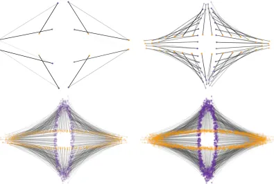
For point sets the optimal transport problem can be solved by a specialized linear pro-gram, the minimum network flow problem (Ahuja et al., 1993; Tarjan, 1997). The minimum network flow problem has been extensively studied in the operations research community and several fast algorithms exist. However, these algorithms, at least on desktop hardware, do not scale beyond a few thousand source and target points. Our framework extends the applications of these algorithms to problem instances several orders of magnitude larger, under suitable assumptions on the geometry of the data. We exploit a multiscale rep-resentation of the source and target sets to reduce the number of variables in the linear program and quickly find good initial solutions, as illustrated in Figure 1. The optimal transport problem is solved (with existing algorithms) at the coarsest scale and the solution is propagated to the next scale and refined. This process is repeated until the finest scale is reached. This strategy, discussed in detail in Section 3, is adaptable to memory limitations and speed versus accuracy trade-offs. For some of the refinement strategies, it is guaranteed to converge to the optimal solution.
Our approach draws from a varied set of work that is briefly summarized in Section 2. The proposed approach generalizes and builds on previous and concurrently developed hierarchical methods (Glimm and Henscheid, 2013; Schmitzer and Schn¨orr, 2013; Schmitzer, 2015; Oberman and Ruan, 2015). The work in this paper adds the following contributions:
• The description of a general multiscale framework for discrete optimal transport that can be applied in conjunction with a wide range of optimal transport algorithms.
strategy based on capacity restrictions of the network flow problem at each scale. This new approach proves to be very efficient and accurate in practice. Overall, the heuristics result empirically in a linear increase in computation time with respect to data set size.
• An implementation in the R package mop that allows the combination of multiple heuristics to tailor speed and accuracy to the requirements of particular applications.
Compared to other linear programming based approaches, the multiscale approach results in a speedup of up to multiple orders of magnitude in large problems and permits to solve approximately transportation problems of several orders of magnitudes larger than previ-ously possible. Comparing to PDE based approaches is difficult and PDE based methods are limited to low-dimensional domains and specific cost metrics. The proposed frame-work is demonstrated on several numerical examples and compared to the state-of-the-art approximation algorithm by Cuturi (2013).
2. Background
Optimal transport is the problem of minimizing the cost of moving a source probability distribution to a target probability distribution given a function that assigns costs to moving mass from source to target locations. The classical formulation by Monge (1781) considers the minimization over mass preserving mappings. Later Kantorovitch (1958) considered the same problem but as a minimization over couplings between the two probability measures, which permits to split mass from a single source across multiple target locations. More precisely, for two probability measuresµandν on probability spacesXand Yrespectively, a coupling of µ and ν is a measure π on X×Y such that the marginals of π are µ and
ν, i.e. π(A× Y) = µ(A) for all (µ-measurable) sets A ⊆ X and π(X ×B) = ν(B) for all (ν-measurable) sets B ⊆ Y. We denote by C(µ, ν) the set of couplings between
µ and ν. Informally, we may think of dπ(x, y) as the amount of infinitesimal mass to be transported from source x to destination y, with the condition that π is a coupling guaranteeing that the source mass is distributed according toµand the destination mass is distributed according toν. Such couplings always exist: we always have the trivial coupling
π =µ×ν. The trivial coupling is uninformative, every source mass dµ(x) is transported to the same target distributionν. In Monge’s formulation the coupling is restricted to the special formπ(x, y) =δT(x) whereδy is the Dirac-δ measure with mass at y∈Y, and T is
a functionX →Y: in this case the coupling is “maximally informative” in the sense that there is a function mapping each source x to a single destinationy; in particular the mass
dµ(x) at x is not split into multiple portions that are shipped to different targety’s. To define optimal transport and optimal couplings, we need a cost function c(x, y) on X×Y representing the work or cost needed to move a unit of mass from xtoy. Then for every coupling π we may define the cost ofπ to be
E(X,Y)∼π[c(X, Y)], (1)
with (X, Y) being a pair of random variables distributed according to π. An optimal coupling π minimizes this cost over all choices of couplings. When seeking an optimal transportation plan, the above becomes
EX∼µ[c(X, T(X))] = Z
X
c(x, T(x))dµ(x),
and one minimizes over all (measurable) functions T : X → Y. One often designs the cost function cin an application-dependent fashion, and the above framework is extremely general. WhenX=Yis a metric space with respect to a distanceρ(with suitable technical conditions relating the metrics and the measuresµ,ν that we will not delve into, referring the reader to Villani (2009)), then distinguished choices for the cost are those that are related to the metric structure. The natural choice of c(x, y) = ρ(x, y)p, for some p > 0
leads to the definition of the Wasserstein-Kantorovich-Rubinstein metric on the space of probability measures on X:
Wp(µ, ν) := min π∈C(µ,ν)
Z
X Z
X
ρ(x, y)pdπ(x, y) 1p
. (2)
transport formulation, briefly discussed in Section 2.1 and, more relevant to this paper, combinatorial optimization methods to directly solve for a discrete optimal transport plan discussed in Section 2.2.
2.1 Continuous Optimal Transport
In case that at least the source distribution admits a density, and when the cost function is the squared Euclidean distance, the optimal coupling is deterministic, i.e. there exists a transport map, and the optimal solution is the gradient of a convex function (Brenier, 1991). This has been exploited to solve the optimal transport problem by numerical partial differential equation approaches (Benamou and Brenier, 2000; Angenent et al., 2003; Haker et al., 2004; Iollo and Lombardi, 2011; Papadakis et al., 2013; Benamou et al., 2014).
An alternative formulation proposed by Aurenhammer et al. (1998) shows that the opti-mal transport from a source density to a target distribution of a set of weighted Dirac delta’s can be solved through a finite dimensional unconstrained convex optimization. M´erigot (2011) proposes a multiscale approach for the formulation of Aurenhammer et al. (1998).
Both the numerical PDE based approaches as well as the unconstrained convex opti-mization require a discretization of the full domain which is generally not feasible for higher dimensional domains. For arbitrary cost functions and distributions the optimal transport problem does typically not result in a deterministic coupling and can not be solved through PDE based approaches.
2.2 Discrete Optimal Transport and Linear Programming
For two discrete distributions µ=Pn1 w(xi)δ(xi) andν =Pm1 v(yi)δ(yi) with Pw(xi) = P
v(yi) = 1 the optimal transport problem is equivalent to the linear program
min
π
X
i=1,...,n j=1,...,m
c(xi, yj)π(xi, yj) s.t.
P
jπ(xi, yj) =µ({xi}) =w(xi) P
iπ(xi, yj) =ν({yj}) =v(yj) π(xi, yj)≥0
. (3)
The solution is called an optimal coupling π∗, and the minimum value attained at π∗, is called the cost of π∗, or the optimal cost of the transport problem, and is denoted by cost(π∗) = P
i,jc(xi, yj)π∗(xi, yj). The constraints enforce that π is a coupling. The
variables π(xi, yj) correspond to the amount of mass transported from sourcexi to target yj, at costc(xi, yj). The linear constraints are of rankn+m−1: when n+m−1 of the
constraints are satisfied, either thenconstraints of the source density or them constraints of the target density are satisfied. Since the sum of outgoing mass is equal to the sum of incoming mass, i.e. µ(X) = ν(Y), it follows that all constraints must be satisfied. The optimal solution lies, barring degeneracies, on a corner of the polytope defined by the constraints, i.e. is a basic feasible solution. This implies that exactly n+m−1 entries of the optimal coupling π are non-zero, i.e. π is a sparse matrix. The optimal coupling is a Monge transport map if and only if all the mass of a sourcexi is transported to exactly one
For source and target data sets with the same cardinality and equally weighted δ -functions, Kantorovich’s optimal transport problem reduces to an assignment problem, whose solution is a Monge optimal transport map. In this special case, the optimal trans-port problem can be efficiently solved by the Hungarian algorithm (Kuhn, 1955). The assignment problem results in a degenerate linear program since onlynentries are non-zero (instead of 2n−1). We can therefore think of optimal transport as a robust version of assignments. This can also be seen from the point of view of convexity: in the assignment problem,π is a permutation matrix deciding to whichyj eachxi is transported. The convex
hull of permutation matrices is exactly the set of doubly-stochastic matrices, to which a couplingπ belongs as a consequence of the constraints in (3).
For point sets with different cardinalities and/or points with different masses the optimal transport problem can be solved by a linear program and is a special case of the minimum cost network flow problem. The minimum cost flow problem is well studied and a number of algorithms (Ford and Fulkerson, 1956; Klein, 1967; Cunningham, 1976; Goldberg and Tarjan, 1987; Bertsekas and Tseng, 1988; Orlin, 1997) exist for its solution. This discrete solution approach is not constrained to specific cost functions and can work with arbitrary cost functions.
However, the linear programming approach neglects possibly useful geometric properties of the measures and the cost function. Our work makes assumptions about the underlying geometry of the measure spaces and the associated cost function, and in this way is a mixing of the low-dimensional “geometric PDE” approaches with the discrete non-geometric optimization approaches. It exploits the geometric assumptions to relieve the shortcomings of either approach, namely it scales to high-dimensional data, provided that the intrinsic dimension is low in a suitable sense, and does not require a mesh data structure. At the same time we use the geometry of the data to speed up the linear program, which per–se does not leverage geometric structures.
The refinement strategies of the proposed multiscale approach add subsets of paths among all pairwise paths at each subsequent scale to improve the optimal transport plan. This strategy of adding paths, is akin to column generation approaches (Desrosiers and L¨ubbecke, 2005). Column generation, first developed by Dantzig and Wolfe (1960) and Ford and Fulkerson (1956), reduces the number of variables in a linear program by solving a smaller linear program on a subset of the original variables and introducing new variables on demand. However, the proposed approach exploits the geometry of the problem in-stead of relying on an auxiliary linear program (Dantzig and Wolfe, 1960) or shortest path computations (Ford and Fulkerson, 1956) to detect the entering variables.
2.3 Approximation Strategies
func-tions, and observing that Lipschitz functions may be characterized by decay properties of their wavelet coefficients. In this sense these approaches are multiscale as well.
To speed up computations in machine learning applications Cuturi (2013) proposes tosmoothtransport plans by adding a maximum entropy penalty to the optimal transport formulation. The resulting optimization problem is efficiently solved through matrix scaling with Sinkhorn fixed-point iterations. Because of the added regularization term, the solution will in general be different from the optimal transportation. It may however be the case that these particular (or perhaps other) regularized solutions are better suited for certain applications.
2.4 Related Work
Very recently a number of approaches have been proposed to solve the optimal transport in a multiscale fashion (Glimm and Henscheid, 2013; Schmitzer and Schn¨orr, 2013; Schmitzer, 2015; Oberman and Ruan, 2015). Glimm and Henscheid (2013) design an iterative scheme to solve a discrete optimal transport problem in reflector design and propose a heuristic for the iterative refinements based on linear programming duality. This iterative scheme can be interpreted as a multiscale decomposition of the transport problem based on geometry of the source and target sets. The proposed potential refinement strategy extends the heuristic proposed by Glimm and Henscheid (2013) to guarantee optimal solutions and adds a more efficient computation strategy: Their approach requires to check all possible variables at the next scale. In Section 3.4.1 we introduce a variation of the approach by Glimm and Henscheid (2013) by adding a branch and bound strategy to avoid checking all variables, and an iterative procedure that guarantees optimal solutions.
Schmitzer and Schn¨orr (2013) propose a multiscale approach on grids that uses a re-finement strategy based on spatial neighborhoods, akin to the neighborhood rere-finement described in Section 3.4.2. Schmitzer (2015) uses a multiscale approach to develop a mod-ified auction algorithm with guaranteed worst case complexity and optimal solutions. We use data structures that enable us to quickly construct neighborhoods, even for point clouds that live in high-dimensions, but have low-intrinsic dimension; we also exploit these struc-tures to not compute all the pairwise possible costs, as well as the candidate neighborhoods in our propagation steps. This can result in substantial savings in the scaling of the algo-rithm, from|X|3to just|X|log|X|. We are therefore able to scale to larger problem, solving on a laptop problems an order of magnitude larger than those in Oberman and Ruan (2015) for example, and showing linear scaling on a large range of scales. Schmitzer (2015) use the c–cyclical monotonicity property of optimal transport plans (Villani, 2009, Chapter 5) to construct “shielding neighborhoods” that permit to exclude paths from further consid-eration. The idea of shielding neighborhoods is combined with a multiscale strategy that permits to quickly refine initial neighborhood estimates.
in a variety of learning tasks; the connections between learning and optimal transportation are still a very open field, to be explored and exploited.
3. Multiscale Optimal Transport
Solving the optimal transport problem for two point setsXand Ydirectly requires |X||Y|
variables, or paths to consider. In other words, the number of paths along which mass can be transported grows quadratically in the number of points and quickly yields exceedingly large problems. The basic premise of the multiscale strategy is to solve a sequence of transport problems based on increasingly accurate approximations of the source and target point set. The multiscale strategy helps to reduce the problem size at each scale by using the solution from the previous scale to inform which paths to include in the optimization at the next finer scale. Additionally, the solution at the previous scale helps to find a good initialization for the current scale which results in fewer iterations to solve the reduced size linear program.
The multiscale algorithm (see Algorithm 1 and Figure 2 for a visual illustration) com-prises of three key elements:
(I) A way of coarsening the sets of source points X and measure µ in a multiscale fashion, yielding a chain
(X, µ) =: (XJ, µJ)→(XJ−1, µJ−1)→ · · · →(Xj, µj)→ · · · →(X0, µ0) (4) connecting the scales from fine to coarse, withXjof decreasing cardinality as the scale
decreases, and the discrete measureµj “representing” a coarsification ofµat scalej,
with supp(µj) = Xj (the support of µj is the set of points with positive measure).
Similarly for Y and ν we obtain the chain
(Y, µ) =: (YJ, νJ)→(YJ−1, νJ−1)→ · · · →(Yj, νj)→ · · · →(Y0, ν0) (5) This coarsening step is described in Section 3.1 and the resulting multiscale family of transport problems is discussed in Section 3.2.
(II) A way ofpropagating a coupling πj solving the transport problem µj νj at scale j to a couplingπj+1 at scalej+ 1. This is described in Section 3.3.
(III) A way of refiningthe propagated solution to the optimal coupling at scalej. This is described in Section 3.4.
3.1 The Coarsening Step: Multiscale Approximations to X, µ and c
Algorithm 1:Multiscale Discrete Optimal Transport
Input: Two discrete measuresµand ν, and a stopping scaleJ0 ≤J Output: Multiscale family of transport plans (πj :µj νj)Jj=00 Construct multiscale structures{{Xj, µj)}Jj=0 and {{Yj, νj)}Jj=0. Let ˜π0 be an arbitrary couplingµ0ν0.
for j= 0. . . J0−1 do
Refine initial guess ˜πj to the optimal coupling πj :µj νj.
Propagateπj from scale j to scale j+ 1, obtaining a coupling ˜πj+1
We start with some notation needed for the definition of the multiscale partitions. Let (X, ρ, µ) be a measure metric space with metric ρ and finite measure µ. Without loss of generality assume thatµ(X) = 1. The metric ball of centerz and radius r isBz(r) ={x∈
X:ρ(x, z)< r}. We say thatXhas doubling dimensiondif every ballBz(r) can be covered
by at most 2d balls of radius r/2 (Assouad, 1983). Furthermore, a space has a doubling
measure if µ(Bz(r)) rd, i.e. if there exist a constant c1 such that for every z ∈ X and
r >0 we havec−11rd≤µ(B
z(r))≤c1rd. Here and in what follows, we say thatf gif there are two constants c1, c2 >0 such that for every z in the domain of both functions f, g we havec1f(z)≤g(z)≤c2f(z) (and therefore a similar set of inequalities holds with the roles of f and g swapped), and we say that f and g have the same order of magnitude. Having a doubling measure implies having a doubling metric, and up to changing the metric to an equivalent one, one may choose the samedin the doubling condition for the metric and in that for the measure: we assume this has been done from now on. This family of spaces is rather general, it includes regular domains inRD, as well as smooth compact manifoldsM
endowed with volume measures.
3.1.1 Multiscale Approximations to X and µ
A regular family of multiscale partitions, with scaling parameter θ >1, is a family of sets
{{Cj,k} Kj
k=1}Jj=0, where j denotes the scale andk indexes the sets at scalej, such that: (i) the sets {Cj,k}
Kj
k=1 form a partition ofX, i.e. they are disjoint and ∪
Kj
k=1Cj,k =X; (ii) eitherCj+1,k0 does not intersect aCj,k, or it is completely contained in it;
(iii) there exists a constantA >0 such that for all j, kwe have the diameter diam(Cj,k)≤ Aθ−j;
(iv) each Cj,k contains a “center” point cj,k such thatBcj,k(θ
−j)⊆C j,k.
To ease the notation we will fix θ = 2 in what follows, but the constructions and results hold, mutatis mutandis, for general θ > 1. The properties (i) and (ii) above imply that there exists a tree T, with nodes at scale j (i.e. at distance j from the root) in bijection with {Cj,k}
Kj
k=1, such that (j+ 1, k
0) is a child of (j, k) if and only if C
j+1,k0 is contained
in Cj,k. Moreover properties (iii) and (iv), together with the properties of spaces with a
doubling measure, imply that µ(Cj,k) 2−jd and Kj 2jd. These partitions are classical
been used to construct multiscale decompositions of data sets in high-dimensions (Little et al., 2012; Allard et al., 2012; Iwen and Maggioni, 2013; Chen et al., 2012). We say that
Cj+1,k0, or even (j+ 1, k0), is a child ofCj,k (respectively, of (j, k)) if Cj+1,k0 ⊆ Cj,k, and
that suchCj,k (respectively (j, k)) is a parent ofCj+1,k0 (resp. (j+ 1, k0)).
Given two discrete setsX and Y in a doubling metric space of homogeneous type with dimensiond, we construct the corresponding families of multiscale partitions{{CX
j,k} KX
j
k=1}Jj=0 and{{CY
j,k} KY
j
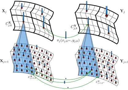
k=1}Jj=0 (we assume the same range of scales to keep the notation simple). The construction of the multiscale approximations is illustrated in Figure 2.
Xj+1
X
jY
jY
j+1CX
j+1,k0
C
j,kXC
Yj,k
⇡j+1(xj+1,k0, yj+1,k00)
CY
j+1,k00
⇡
j(
x
j,k000, y
j,k)
Figure 2: An illustration of the multiscale framework. The coarsening step constructs from a set of weighted points Xj+1 at scale j+ 1 a smaller set of weighted points at scalej (blue bars). An equivalent coarsening is performed on the target point set Yj+1Neighboring points at scalej+1 are combined into a single representative at scalejwith mass equivalent to the weights of the combined points. The optimal transport plan (green arrows) is solved at the coarser scalej, then propagated to scalej+ 1 and refined.
The space Xj will be the partition at scale j, namely the set {Cj,kX} KX
j
k=1, of cardinality
KX
recursively onXj by
µj(Cj,kX) =
X
(j+1,k0) child of (j,k)
µj+1(CjX+1,k0), (6)
and similarly forνj. These are in fact projections of these measures, and may also be
inter-preted as conditional expectations with respect to theσ-algebra generated by the multiscale partitions. We can associate a point cX
j,k to each Cj,kX in various ways, by “averaging” the
points in CX
j+1,k0, for (j+ 1, k0) a child of (j, k). At the finest scale we may let cXJ,k =cXJ,k
(this being a “center” forCJ,k as in item (iv) in the definition of multiscale partitions), and
then recursively we defined the coarser centers step from scalej+ 1 to scale j in one of the following ways:
(i) If the metric space is also a vector space a natural definition ofxj,k :=cXj,kis a weighted
average of thecX
j+1,k0 corresponding to children: cX
j,k =
X
(j+1,k0) child of (j,k)
µj+1({cXj+1,k0})cXj+1,k0.
(ii) In general we can definexj,k :=cXj,k as the point
cX
j,k = argminc∈X
X
(j+1,k0) child of (j,k)
ρp(c, cX j+1,k0),
for somep≥1, typicallyp= 1 (median) or p= 2 (Fr´echet mean).
Of course similar constructions apply to the space Yj, yielding points yj,k := cYj,k. We
discuss algorithms for these constructions in Section 4.1.1.
3.1.2 Coarsening the cost function c
The multiscale partition provides several ways to coarsen the cost function: for every xj,k
and yj,k0 we consider
(c-i) the pointwise value
cj(cXj,k, cYj,k0) :=c(xXj,k, yYj,k0), (7)
wherexj,k and yj,k0 are defined in any of the ways above;
(c-ii) the local average
cj(cXj,k, cYj,k0) := argmin α
X
x∈CX
j,k, y∈Cj,kY0
(α−c(x, y))2 =
P x∈CX
j,k, y∈CYj,k0
c(x, y)
|CX j,k||Cj,kY0|
; (8)
(c-iii) the local weighted average
cj(cXj,k, cYj,k0) := argmin α
X
x∈CX j,k, y∈C
Y j,k0
(α−c(x, y))2π∗j−1(xj−1,k1, yj−1,k01)
=
P x∈CX
j,k, y∈Cj,kY0
c(x, y)π∗
j−1(xj−1,k1, yj−1,k10)
P x∈CX
j,k, y∈Cj,kY0π ∗
j−1(xj−1,k1, yj−1,k01)
whereπ∗
j−1 is the optimal or approximate transportation plan at scale j−1, defined in (9);k1 is the unique index for which Cj,kX ⊆CjX−1,k1 and k
0
1 is the unique index for which CY
j,k ⊆CjY−1,k10 .
3.2 Multiscale Family of Optimal Transport Problems
With the definitions of the multiscale family of coarser spaces Xj and Yj, corresponding
measures µj and νj, and corresponding cost cj, we may consider, for each scale j, the
following optimal transport problem:
πj∗ := argmin
π
X
k=1,...,KX j
k0=1,...,KY j
cj(xj,k, yj,k0)π(xj,k, yj,k0) s.t. P
k0π(xj,k, yj,k0) =µj({xj,k}) ∀k∈KX j P
kπ(xj,k, yj,k0) =νj({yj,k0}) ∀k0 ∈KjY π(xj,k, yj,k0)≥0
(9) The problems in this family are related to each other, and to the optimal transportation problem in the original spaces. We define the cost of a coupling as
cost(πj) = X
k=1,...,KjX k0=1,...,KY j
cj(xj,k, yj,k0)πj(xj,k, yj,k0). (10)
The cost of the optimal coupling πj∗ at scale j is provably an approximation to the cost of the optimal coupling π∗ (which is equal to πJ∗):
Proposition 1 Let π∗ be the optimal coupling, i.e. the solution to (3), andπ∗j the optimal coupling at scale j, i.e. the solution to (9). Define
Ej(π∗) := X
k=1,...,KX j
k0=1,...,KY j
X
x∈CX j,k
y∈CY j,k0
cj(xj,k, yj,k0)−c(x, y)π∗(x, y). (11)
Then
cost(πj∗)≤cost(π∗) +Ej(π∗), (12)
and if cj =cand cis Lipschitz with constant ||∇c||∞, we have
cost(πj∗)≤cost(π∗) + 2−jA||∇
c||∞, (13)
where A is such that maxk,k0{diam(CX
j,k),diam(Cj,kY0)} ≤A·2−j.
Proof Consider the couplingπj induced at scalej by the optimal coupling π∗, defined by
πj(xj,k, yj,k0) =
X
x∈CX j,k,y∈C
Y j,k0
First of all, since{CX
j,k}k and {Cj,kY0}k0 are partitions, it is immediately verified that πj is a
coupling. Secondly, observe that
cost(πj) = X
k=1,...,KX j
k0=1,...,KY j
cj(xj,k, yj,k0)πj(xj,k, yj,k0) = X
k=1,...,KX j
k0=1,...,KY j
X
x∈CX j,k
y∈CYj,k0
cj(xj,k, yj,k0)π∗(x, y)
= X
x∈X y∈Y
c(x, y)π∗(x, y) + X
k=1,...,KX j
k0=1,...,KY j
X
x∈CX j,k
y∈Cj,kY0
cj(xj,k, yj,k0)−c(x, y)π∗(x, y)
=cost(π∗) + X
k=1,...,KX j
k0=1,...,KY j
X
x∈CX j,k
y∈CY j,k0
cj(xj,k, yj,k0)−c(x, y)π∗(x, y)
| {z }
=:Ej(π∗)
.
Since cost(π∗
j) ≤ cost(πj) (since πj∗ is optimal), we obtain (12). When cj = c and c is
Lipschitz with constant||∇c||∞, we have
Ej(π∗)≤ X
k:x∈CX j,k
k0:y∈CY j,k0
X
k=1,...,KX j
k0=1,...,KY j
||∇c||∞· ||(xj,k, yj,k0)−(x, y)||π∗(x, y)
≤ X
k:x∈CX j,k
k0:y∈CY j,k0
X
k=1,...,KX j
k0=1,...,KY j
||∇c||∞2−jAπ∗(x, y)
≤2−jA||∇c||∞,
withA as in the claim.
In the discrete, finite case that we are considering, µj → µ and νj → ν trivially since µJ = µ and νJ = ν by construction. If µ and ν were continuous, and at least when
c(x, y) =ρ(x, y)p for somep≥1, then if µand ν have finite p-moment (i.e. R
Xρ(x, x0) pdµ
and similarly for ν), we would obtain convergence of a subsequence of c(π∗
j) to c(π∗) by
general results (e.g. as a simple consequence of Lemma 4.4. in (Villani, 2009)).
Note that the approximations do not guarantee that the transport plans are close in any other sense but their cost. Consider the arrangement in Figure 3, the transport plans are -close in cost but the distances between the target locations of the sources are far no matter how small gets.
3.3 Propagation Strategies
The approximation bounds in Section 3.2 show that the optimal solution πj at scale j is
|Ej+1−Ej|close to optimal solutionπ∗j+1 at scale j+ 1. This suggests that the solution at
scalej can provide a reasonably close to optimal initialization for scale j+ 1.
1
1
Y B
Z A
1
1
Y B
Z A
(a) (b)
Figure 3: An example that illustrates that closeness in cost does not indicate closeness of the transport plan. The transport plans (green arrows) between the sources A and B (purple) and the targets Y and Z (orange) in (a) and (b) are -close but their respective target locations are very far.
transport problem at scale j+ 1 given the solution πj∗ at scale j is to distribute the mass
π∗
j(xk, yk0) equally to all combinations of paths between children(xk) and children(yk0).
This propagation strategy results in a reduction in the number of iterations required to find an optimal solution at the subsequent scale. This warm-starting alone is often not sufficient, however. At the finest scale the problems still requires the solution of a problem of size O(n2). This quickly reaches memory constraints with Ω(104) points, and a single iteration of Newton’s method or a pivot step of a linear program becomes prohibitively slow. Thus, we consider reducing the number of variables, which substantially speeds up the algorithm, albeit we may lose guarantees on its computational complexity and/or its ability to achieve arbitrary accuracy, so that only numerical experiments will support our constructions. These reductions are achieved by considering only a subset Rj+1 of all possible pathsAj+1 at scalej+ 1.
To distinguish the optimal solution on the reduced set of paths at scale j from the optimal solution over all paths we introduce some notation. Let Aj+1 be the set of all possible paths between sources and targets at scale j+ 1. LetRj+1 ⊆Aj+1 be the set of paths propagated from the previous solution (e.g. children of mass-bearing paths found at scalej). Letπ∗
j+1|P be the optimal solution to the transport problem restricted to a set of
paths P ⊂Aj+1. With this notation, πj∗+1|Aj+1 =π
∗
j+1. The optimal coupling πj∗+1|Rj+1
on the reduced set of paths problem does not need to match the optimal couplingπj∗+1 on all paths. Howeverπ∗
j+1|Rj+1 does provide a starting point for further refinements discussed in Section 3.4.
3.3.1 Simple Propagation
mass-bearing paths at scale j. The optimal solution at scale j has exactly KX
j +KjY−1 paths
with non-zero weight. Thus, the number of paths at scalej+1 reduces toO(C2(KX
j +KjY)),
whereCis the maximal number of children of any node at scalej. In particular,C2dfor
a doubling space of dimension d. This reduces the number of variables from “quadratic”,
O(KX
j KjY), to linear, O(KjX+KjY). This propagation strategy by itself, however, often
leads to a dramatic loss of accuracy in both the cost the transportation plan, and the transportation plan itself.
3.3.2 Capacity Constraint Propagation
This propagation strategy solves a modified minimum flow problem at scale j in order to include additional paths at scalej+ 1 that are likely to be included in the optimal solution
πj∗+1. This is achieved by adding a capacity constraint to the mass bearing paths at scalejin the optimal couplingπ∗
j|Rj: The amount of mass of a mass bearing pathπ ∗
j|Rj(xj,k, yj,k0) is constrained toλmin µj(xj,k), νj(yj,k0) withλrandom uniform on [0.1,0.9]. The
random-ness is introduced to avoid degenerate constraints. The solution of this modified minimum– flow problem forces the inclusion of nc additional paths, where nc is the number of
con-straints added. There are various options for adding capacity concon-straints, we propose to constrain all mass bearing paths of the optimal solution at scale πj∗|Rj. The capacity con-strained problem thus results in a solution with twice the number of paths as in the coupling
πj∗|Rj. The solution of the capacity constrained minimum flow problem is propagated as before to the next scale.
To increase the likelihood of including paths required to find an optimal solution at the next scale, the capacity constrained procedure can be iterated multiple times. Each time the mass bearing paths in the modified solution are constrained and a new solution is computed. Each iteration doubles the number of mass bearing paths and the number of iterations controls how many paths are propagated to the next scale. Thus, the capacity constraint propagation strategy bounds the number of paths considered in the linear program. The optimal transport plan on a source setX andY results in a linear program with |X|+|Y|
constraints and |X||Y| variables and the optimal transport plan has |X|+|Y| −1 mass bearing paths. It follows that the capacity constraint propagation strategy considers linear programs with at most O 2i(|X|+|Y|)
constraints, where i is the number of iterations of the capacity propagation scheme. This results in a significant reduction in problem size, since at each scale we only consider a number of paths scaling as O(|X|+|Y|) instead of
O(|X||Y|).
3.4 Refinement Strategies
3.4.1 Potential Refinement
This refinement strategy exploits the potential functions, or dual solution, to determine additional paths to include given the currently optimal solution on the reduced set of paths from the propagation. The dual formulation of the optimal transport can be written as:
max
φ,ψ X
i=1,...,n
µ({xi})φ(xi)− X
j=1,...,m
ν({yj})ψ(yj) s.t. φ(xi)−ψ(yj)≤c(xi, yj). (14)
The functionsφandψare called dual variables or potential functions. From the dual formu-lation it follows that at an optimal solution thereduced costc(x, y)−φ(x) +ψ(y) is larger or equal to zero. This also follows from the Kantorovich duality of optimal transport (Villani, 2009, Chapter 5).
The potential refinement strategy uses the potential functionsφandψfrom the solution of the reduced problem to determine which additional paths to include. If the solution on the reduced problem is not optimal on all paths, then there exist paths with negative reduced cost. Thus, we check the reduced cost between all paths and include the ones negative reduced cost. A direct implementation of this strategy would require to check all possible paths between the source and target points. To avoid checking all pairwise paths between source and target point sets at the current scale, we introduce a branch and bound procedure on the multiscale structure that efficiently determines all paths with negative reduced cost.
Letφ∗j|Pandψj∗|Pthe dual variables, i.e., the potential functions, at the optimal solution
π∗
j|P on the set of paths P for the source and target points, respectively. DefineVj(π∗j|P)
as the set of paths with non-positive reduced cost with respect to φ∗j|P and ψ∗j|P
Vj(πj∗|P) =
πj(xk, yk0)∈Aj :c(xk, yk0)−φ∗j|P(xk)−ψj∗|P(yk0)≤0 .
The potential refinement strategy now refines the propagated solution π∗j|Rj by including all negative reduced cost paths Q0
j = Vj(π∗j|Rj). Let π ∗
j|Q0
j be the associated optimal transport. This new solution changes the potential functions which in turn may require to include additional paths. Thus the potential refinement strategy can be iterated with Qi
j =Vj(πj∗|Qij−1) leading to monotonically decreasing optimal transport plansπ
∗
j|Qi
j. Since a solution is optimal if and only if all reduced cost are≥0 this iterative strategy converges to the optimal solution.
The set of paths with negative reduced cost given φ∗
j|P and ψ∗j|P are determined by
descending the tree and excluding nodes that can not contain any negative reduced cost paths. This requires bounds on the potential functions for any node at scale smaller than
j. The bound is achieved by storing at each target node of the multiscale decomposition the maximal ψ∗j|P of any of its descendants at scale j. Now for each source node xk the
target multiscale decomposition is descended, but only towards nodes at which a potential negative reduced cost can exist.
Depending on the properties ofφ∗j|Pand ψj∗|P, this refinement strategy may reduce the number of required cost function evaluations drastically. In empirical experiments the total number of paths considered in the iterative potential refinement was typically reduced to
O(2d(KX
The potential refinement strategy is also employed by Glimm and Henscheid (2013) with-out the branch and bound procedure. The shielding neighborhoods proposed by Schmitzer (2015) similarly uses the potentials to define which variables are needed to define a sparse optimal transport problem and also suggests to iterate the neighborhood shields in order to arrive at an optimal solution.
3.4.2 Neighborhood Refinement
This section presents a refinement strategy that takes advantage of the geometry of the data. The approach is based on the heuristic that most paths at the next scale are sub-optimal due to boundary effects when moving from one scale to the next, induced by the sharp partitioning of the space at scalej. Such artifacts from the multiscale structure are mitigated by including paths between spatial neighbors in the source and target locations of the optimal solution on the propagated paths. This refinement strategy is also employed by Oberman and Ruan (2015).
Let Nj(πj, r) be the set of paths such that the source and target of any path are
within radius r of the source and target of a path with non-zero mass transfer in πj. The
neighborhood refinement strategy is to expand the reduced set of paths using the union of paths in the current reduced set and its neighbors:
Ej =Rj∪Nj π∗j|Rj, r
When moving from one scale to the next the cost of any path can change at most two times the radius r of the parent node which suggests to set the radius of the neighborhood in consideration as two times the node radius.
This heuristics does not guarantee an optimal solution, but does reduce the number of paths to consider at scale j to O(q2
r(KjX+KjY)) with qr being the number of neighbors
within radius 2−jr, for a doubling space with dimensiond,q rrd.
The neighborhood strategy requires to efficiently compute the set of points within a ball of a given radius and location. Depending on the multiscale structure there are different ways to compute the set of neighbors. A generic approach that does not depend on any specific multiscale structure is to use a branch and bound strategy. For this approach, each node requires an upper bound u(ci) on the maximal distance from the representative of
node ci to any of its descendants. Using these upper bounds the tree is searched, starting
from the root node, while excluding any child nodes for which c(x, ci)−u(ci) > r from
further consideration. For multiscale structures such as regular grids more efficient direct computations are possible. For this paper we implemented the generic branch and bound strategy that works with any multiscale structure.
3.5 Remark on Errors
might not be optimal. This second type error is difficult to quantify; however, for the potential refinement strategy that we introduce Section 3.4.1, an optimal solution can be guaranteed. The propagation and refinement strategies introduced in Sections 3.3 and 3.4 permit trade-offs between accuracy and computational cost.
4. Numerical Results and Comparisons
We tested the performance of the proposed multiscale transport framework with respect to computational speed as well as accuracy for different propagation and refinement strategies on various source and target point sets with different properties.
The multiscale approach is implemented in C++ with an R front end in the package
mop1. For comparisons, we also implemented the Sinkhorn distance approach (Cuturi, 2013) in C++ with an R front end in the package sinkhorn1. Our C++ implementation uses the Eigen linear algebra library (Guennebaud et al., 2010), which resulted in faster runtimes than the MATLAB implementation by Cuturi (2013).
4.1 Implementation Details
The Rpackage mop provides a flexible implementation of the multiscale framework and is adaptable to any multiscale decomposition that can be represented by a tree. The package permits to use different optimization algorithms to solve the individual transport prob-lem. Currently the multiscale framework implementation supports the open source library GLPK (Makhorin, 2013) and the commercial packages MOSEK (Andersen and Andersen, 2013) and CPLEX (IBM, 2013) (both free for academic use). MOSEK and CPLEX support a specialized network simplex implementation that runs 10-100 times faster than a typical primal simplex implementation. Both the MOSEK and CPLEX network simplex run at comparable times, with CPLEX slightly faster in our experiments. Furthermore CPLEX supports starting from an advanced initial basis for the network simplex algorithm which improves the multiscale run-times significantly. Thus, the numerical test are all run using the CPLEX network simplex algorithm.
4.1.1 Algorithms for Constructing Multiscale Point Set Representations
Various approaches exist to build the multiscale structures described in Section 3.1, such as hierarchical clustering type algorithms (Ward Jr, 1963), or in low dimensions constructions such as quad and oct-trees (Finkel and Bentley, 1974; Jackins and Tanimoto, 1980) or kd-trees (Bentley, 1975) are feasible. Data structures developed for fast nearest neighbor queries, such as navigating nets (Krauthgamer and Lee, 2004) and cover trees (Beygelzimer et al., 2006) induce a hierarchical structure on the data sets with guarantees on partition size and geometric regularity of the elements of the partition at each scale, under rather general assumptions on the distribution of the points. The complexity of cover trees (Beygelzimer et al., 2006) is O(CdDnlogn), for some constant C, where n = |X|, d is the doubling
dimension of X, and D is the cost of computing a distance between a pair of points. Therefore the algorithm is practical only when the intrinsic dimension is small, in which case they are provably adaptive to such intrinsic dimension. The optimal transport approach
does not rest on a specific multiscale structure and can be adapted to application-dependent considerations. However, the properties of the multiscale structure, i.e., depth and partition sizes, do affect run-time and approximation bounds.
In our experiments we use an iterative K-means strategy to recursively split the data into subsets. The tree is initialized using the mean of the complete data set as the root node. Then K-means is run resulting in K children. This procedure is recursively applied for each leaf node, in a breadth first fashion, until a desired number of of leaf nodes, a maximal leaf radius or the leaf node contains only a single point. For the examples shown we select K = 2d with d the dimensionality of the data set. For high-dimensional data K could be set to an estimate of the intrinsic dimensionality. Since in all experiments we are equipped with a metric structure we use the pointwise coarsening of the cost function as in Equation (7). The reported results include the computation time for building the hierarchical decomposition, which is, however, negligible compared to solving the transport problem at all scales.
4.1.2 Multiscale Transport Implementation for Point Sets
Algorithm 2 details the steps for computing multiscale optimal transport plans using the newtork simplex for solving the optimization problems at each scale and iteratedK–means to construct the multiscale structures.
Algorithm 2:Point Set based Multiscale Optimal Transport Implementation Input: Source point setX={x}N
i=0. Target point set Y={y}M
i=0. A propagation strategyp. A refinement strategy r.
Output: Multiscale family of transport plans (πj :Xj Yj)Jj=0
Construct multiscale point sets {Xj}Nj=0 and {Yj}Mj=0 using iterated K–means. if N < M then
Add scales{Xj}Jj=N+1 by repeating the last scale. if N > M then
Add scales{Yj}Jj=M+1 by repeating the last scale. Set J = max(N, M)
Form the measures µj and νj as in equation (6).
Compute optimal transport π0 at coarsest scale with the network simplex. for j= 1. . . J do
Propagate theπj−1 from scale j−1 to scale j using the propagation strategy p, obtaining a set of pathsSj =p(πj−1 at scalej
Use the network simplex algorithm to solve for optimal transport on the set of pathsSj yielding a coupling ˜πj
Create the refined set of pathsRj =r(˜πj) using the refinement strategyr.
4.2 Propagation and Refinement Strategy Performance
Figure 5 illustrates the behaviour of the different propagation and refinement strategies on two examples: The ellipses example in Figure 1 and Caffarelli’s smoothness counter example described in Villani (2009, Chapter 12) and illustrated in Figure 4. The ellipse example consists of two uniform samples (source and target data set) of sizen from the unit circle with normal distributed noise added with zero mean and standard deviation 0.1. The source data sample is then scaled in the x-Axis by 1.3 and in the y-Axis by 0.9, while the target data set is scaled in the x-Axis by 0.9 and in the y-Axis by 1.1. Caffarelli’s example consists of two uniform samples on [−1,1]2 of size n. Any points outside the unit circle are then discarded. Additionally, the target data sample is split along the x-Axis at 0 and shifted by +2 and −2 for points with positive and negative x-Axis values, respectively. We tested 7
(a) (b)
Figure 4: Optimal transport plans on the (a) ellipse and (b) Caffarelli data sets with 5000 points for the source and target point set each. The optimal transport plans are indicated by black lines with transparency indicating the amount of mass being transported from source to target.
different strategies of different combinations of propagation strategies from Section 3.3 with refinement strategies from Section 3.4:
1. (ICP) Iterated capacity propagation (Section 3.3.2) with 0 to 5 iterations with no re-finements. Note iterated capacity with 0 iterations is equivalent to simple propagation (Section 3.3.1).
2. (NR) Simple propagation (Section 3.3.1) with neighborhood refinement (Section 3.4.2) with radius factor ranging from 0.5 to 2.5 in 0.5 increments.
3. (ICP + NR) Iterated capacity propagation with 1 to 5 iterations combined with neighborhood refinement with radius factor fixed to 1.
4. (CP + NR) A single iteration of capacity propagation combined with neighborhood refinement with radius factor from 0.5 to 2.5 with 0.5 increments.
5. (IPR) Simple propagation with iterated potential refinement (Section 3.4.1) with 1 to 5 iterations.
6. (ICP + PR) Iterated capacity propagation with 1 to 5 iterations combined with a single potential refinement step.
Figure 5 shows that almost all strategies have less than one percent relative error. The exception is the simple propagation with no refinements applied (i.e. iterated capacity prop-agation with no iterations). The randomness of the iterated capacity constrained algorithm can results in worse results despite a larger number of iterations. However, it will always perform better than using the simple propagation strategy. The neighborhood refinement strategy improves the results significantly, but after a radius factor of one the improvements start to level out. The potential refinement strategy finds the optimal solution when iter-ated a few times. Combining the refinement strategy with capacity propagation reduces relative error and computation time. The computation time is reduced because the capac-ity propagation yields a closer initialization to the optimal solution. The combination of potential refinement strategy and capacity propagation has the additional benefit that the branch and bound strategy is more efficient since fewer comparisons need to be made when checking for paths and smaller linear programs have to be solved in each refinement step. For very small relative error (< 10−11) the optimal solution is sometimes not achieved.
(a) (b)
Figure 5: A comparison of different multiscale propagation and refinement strategies on the (a) ellipse and (b) Caffarelli data sets with 5000 points for the source and target point set each. For a description of the different strategies see text, the lines in the relative error graphs indicate increasing number of iterations or radius factor for the different strategies. Both the time and accuracy axes are in logarithmic scale. All strategies, except capacity propagation with 0 iterations (ICP) and neighborhood refinement (NR) with radius factor 0.5, find solution with relative error less than one percent. The capacity propagation strategies can find optimal solutions up to numerical precision.
This is due to tolerance settings in the network simplex algorithm which are on the order of 10−11. Thus, depending how the network simplex approaches the optimum it might stop at different basic feasible solutions.
the transport distance to the diameters of the source and target point sets. To illustrate this effect we computed optimal transport plans for two data sets with source and target distributions uniform on [0,1]2. In the first case the distributions are perfectly overlapping and in the second case the target distributions shifted by 2 units in the x direction. Figure 6 shows that for large ratios the relative error is typically much smaller. This is expected since variations in the transport plan only change the cost marginally. For small ratios, i.e. source and target distributions that are almost identical, a small variation in the transport plan leads to a large relative error. Another observation is the following: the potential strategy
(a) (b)
Figure 6: The effect of distance to support size ratio on computation time and relative error for the different multiscale propagation and refinement strategies source and target point sets of 5000 points each sampled uniformly from a square of side length one and ground truth transport distance (a) 0 and (b) 2. Both the time and accuracy axes are in logarithmic scale.
is less effective for transport problems where most mass is transported very far, relative to the distances within source and target point set. This is because a small change in the length of a path can include many possible source and target locations and the transport polytope has many suboptimal solutions with similar cost. If on the other hand most mass is transported on the order of the nearest neighbor distances within the source and target point set, there are many fewer possible paths within a small change in path length and the transport polytope is “steep” in the direction of the cost function.
4.3 Comparison to Network Simplex and Sinkhorn Transport
In this section we compare the CPLEX network simplex algorithm (IBM, 2013) and the Sinkhorn approach (Cuturi, 2013) to three different multiscale strategies:
2. (CP + NR) Capacity propagation combined with neighborhood refinement with radius factor fixed to one and a single capacity constraint iteration.
3. (CP + PR) Capacity propagation combined with potential refinement with a single iteration each.
(a) (b)
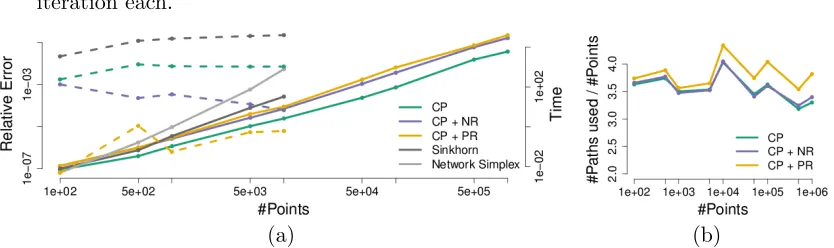
Figure 7: (a) A comparison of computation time (solid) and relative error ( dashed ) with respect to the network simplex solution for the CPLEX network simplex, Sinkhorn distance and the proposed multiscale strategy with increasing number of points. (b) The number of total paths considered is roughly constant with four times the number of points in the problem, i.e., the multiscale approach results in only a linear increase in problem size instead of quadratic for a direct approach. The number of points on the x-axis denotes the number of source points|X|which is approximately equal to the number of target points|Y|. The Sinkhorn approach is competitive in computation time for smaller problems. For larger problems only the multiscale strategies outperform the Sinkhorn approach quickly, and are the only algorithms that remain viable.
The relative error and computation time depend again on the type of problem. Fig-ure 8(a) shows computation time and relative error on transport problems on source and target data sets sampled uniformly from [0,1]2 with different shifts in the target distribu-tion. If required, the relative error can be reduced using multiple capacity propagation and potential refinement iterations as illustrated in Figure 6. In these experiments we set the tolerance parameter for Sinkhorn to 1e−5, and tried also 1e−2 to see if this would result in significant speed ups, with minimal accuracy loss, but it resulted in only approximately a 10% speedup, and no fundamental change in the behavior for large problem sizes. The tolerance parameter for CPLEX is set to 1e−8. The approach by Schmitzer (2015) is similar to the refinement property strategy, we expect that computation time grows similarly as for the potential strategy for problems with large transport distances compared to the source and target support size.
The final experiment tests the performance with respect to the dimensionality of the source and target distributions. We used two uniform distributions [0,1]d with d varying
from 2 to 5 and the target shifted such that the actual transport distance is 0 and 2.
(a) (b) (c)
Figure 8: Computation time (solid) and relative error (dashed) with respect to (a) changes transport distance to support size ratio in two dimensions and (b,c) dimensionality with ground truth transport distance (b) 0 and (c) 2. The source and target distributions are uniform on a square of side length 1 with approximately 5000 points each. The potential refinement increases proportional to the transport distance to support ratio. The neighborhood strategy is less effective in higher dimensions, due to the curse of dimensionality, but performs better than the Sinkhorn approach. The capacity propagation strategy is less affected by the dimensionality of the problem.
5. Application to Brain MR Images
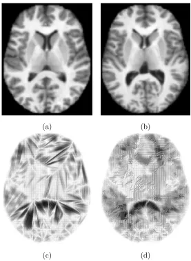
To solve for the optimal transport map between two 3D brain images we extract for each image a point cloud from the intensity volumes. Each point represents a voxel as a point in 3-dimensional space, the location of the voxel. The mass of the point is equal to the intensity value of the voxel, normalized to sum to one over all points. For illustration, Figure 9 shows a single slice extracted from the original volumes and optimal transport maps between the two slices. This 2D problem resulted in point set of approximately 20,000 points.
(a) (b)
(c) (d)
Figure 9: Slice of (a) source and (b) target brain image and optimal transport map for (c) Euclidean and (d) squared Euclidean cost function. For the squared Euclidean cost the optimal transport solutions typically prefer to move many locations small distances, i.e. shift mass among nearest neighbors. For images the neighborhoods are on regular grids resulting in a staircase appearance of the transport plan.
Model Residual R2 F–statistic p–value
age =a0+P5i=1aili 10.5 0.82 404.9 <
age =a0+P3i=1aixi 10.87 0.82 639.5 <
age =a0+P5i=1aizi 12.04 0.78 297 <
age =a0+a1z11+a2z21+a3z12+a4z22+a5z31+a6z24+a7z45+a8z51 10.9 0.82 239 <
MMSE =a0+a1age 3.59 0.06 15.82 9.3e-05
MMSE =a0+a1l1 3.40 0.16 43.13 3.3e-10
MMSE =a0+a1x1 3.36 0.18 50.30 1.6e-11
MMSE =a0+a1z1+a2z3+a3z5 3.38 0.17 16.31 1.2e-09
MMSE =a0+a1z22+a2z23+a3z34+a4z54+a5z15+a6z53+a7z36 3.14 0.30 14.03 4.3e-15
CDR =a0+a1age 0.27 0.25 144.5 <
CDR =a0+a1l1 0.26 0.34 223.9 <
CDR =a0+a1x1 0.25 0.36 248.5 <
CDR =a0+a1z1+a2z3+a3z5 0.26 0.35 77.5 <
CDR =a0+a1z34+a2z15+a3z53+a4z55+a5a63 0.25 0.38 53.1 <
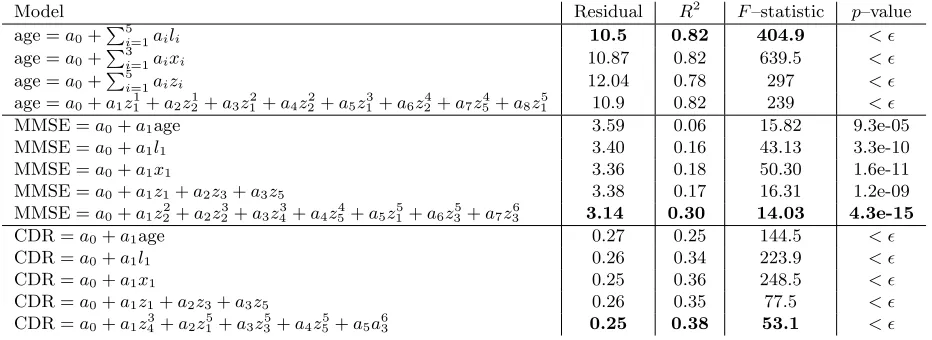
Table 1: Optimal linear regression models from the OASIS data set, for age, mini mental state examination (MMSE) and clinical dementia rating (CDR). The PCA coordi-nates from the Euclidean distances are denoted withli, the diffeomorphic manifold
coordinates withxi, the transport coordinates by zi and the multiscale transport
coordinates withzij from coarsestj= 1 to finestj= 6 scale. An entry with “< ” denotes quantities smaller than machine precision. The best results are indicated in bold.
Euclidean space. In this embedding each point corresponds to a 3D brain image and thus provides a coordinate system for the relative locations between the brain MRI’s. The Euclidean structure of the embedding permits to use standard statistical tools to form prediction models, in our case linear regression.
Within this framework we compare Euclidean, LDDMM and optimal transport distances as the input to the multidimensional scaling step. Note, for the Euclidean distance, i.e. treating each brain MRI as a point in Euclidean space, classical multidimensional scaling is equivalent to a principal component analysis. For the comparisons we used the OASIS brain database (HHMI et al.). The OASIS database consists of T1 weighted MRI of 416 subjects aged 18 to 96. One hundred of the subjects over the age of 60 are diagnosed with mild to moderate dementia. The images in the OASIS data set are already skull-stripped, gain-field corrected and registered to the atlas space of Talairach and Tournoux (1988) with a 12-parameter affine transform. Associated with the data are several clinical 12-parameters. For the linear regression from the MDS embeddings we restrict our attention to the prediction of age, mini mental state examination (MMSE) and clinical dementia rating (CDR).
The MDS computation requires pairwise distances. To speed up computations we reduce the number of points by downsampling the volumes to size 44×52×44. This results, discarding zero intensity voxels, in point clouds of approximately 40,000 points for each brain MRI. A single distance computation with capacity propagation takes on the order of 10 seconds resulting in a total computation time of around 2 weeks for all pairwise distances. For embedding the optimal transport distance we consider two approaches:
2. A multiscale embedding using multiple five dimensional MDS embeddings, one for the transport cost at each scale.
From the embeddings we build linear regression models, using the embedding coordi-nates as independent variables and the clinical variables as dependent variables. As in Ger-ber et al. (2010) we use the Bayesian information criterion (BIC) on all regression subsets to extract a models that trade-off complexity, i.e. number of independent variables, with the quality of fit. Table 1 shows the results of the optimal transport, with squared Euclidean cost, distances compared to the results reported in Gerber et al. (2010). The transport based approach shows some interesting behaviours. The single scale model performs worse on age while performing similar on MMSE and CDR. The multiscale transport models perform similar to the LDDMM approach except for MMSE where it almost doubles the explained variance R2. This suggests that the multiscale approach captures information about MMSE not contained in a single scale and prompts further research of multiscale based models to predict clinical parameters.
6. Conclusion
The multiscale framework extends the size of transport problems that can be solved by linear programming by one to two orders of magnitude in the size of the point sets.
The framework is flexible, the linear program at each scale can be solved by any method. Depending on the refinement strategy a dual solution would need to be constructed as well. The method can also be applied to solve the linear assignment problem. The solution at the finest scale will be binary if n = m, however, at intermediate steps a binary solution is not guaranteed unless at each scale the source and target sets have the same number of points. This could be enforced during the construction of the multiscale structures. As currently defined the method requires point set inputs for the multiscale constructing of the transport problems. However, one could design methods that construct such a multiscale structure from a cost matrix only. However, for large problems pairwise computations of all costs is typically prohibitively expensive.
The multiscale transport framework provides several options for further research. The framework can be combined with various regularizations, e.g. depending on scale and location and induces a natural multiscale decomposition of the transport map. This de-composition can be used to extract information about relevant scales in a wide variety of application domains. We are currently investigating the use of such multiscale decomposi-tions for representation and analysis of sets of brain MRI.
The capacity constraint propagation approach suggests a different venue for further exploration. The capacity propagation strategy does not hinge on a geometrical notion of neighborhoods and is a suitable candidate to extend the multiscale framework to non-geometric problems. Studying the interdependency between the cost function, hierarchical decomposition of the transport problem (or possibly more generic linear programs) and the efficiency of the capacity constraint propagation is a challenging but interesting problem.
We thank the referees for their constructive feedback. This work was supported, in part, by NIH/NIBIB and NIH/NIGMS via 1R01EB021396-01A1: Slicer+PLUS: Point-of-Care Ultrasound.
References
Ravindra K. Ahuja, Thomas L. Magnanti, and James B. Orlin. Network Flows: Theory, Algorithms, and Applications. Prentice-Hall, Inc., Upper Saddle River, NJ, USA, 1993. ISBN 0-13-617549-X.
William K Allard, Guangliang Chen, and Mauro Maggioni. Multi-scale geometric meth-ods for data sets ii: Geometric multi-resolution analysis. Applied and Computational Harmonic Analysis, 32(3):435–462, 2012.
Erling D. Andersen and Knud D. Andersen. The MOSEK optimization software. http://www.mosek.com/, 2013.
Alexandr Andoni, Piotr Indyk, and Robert Krauthgamer. Earth mover distance over high-dimensional spaces. In Proceedings of the nineteenth annual ACM-SIAM symposium on Discrete algorithms, pages 343–352. Society for Industrial and Applied Mathematics, 2008.
Sigurd Angenent, Steven Haker, and Allen Tannenbaum. Minimizing flows for the monge– kantorovich problem. SIAM journal on mathematical analysis, 35(1):61–97, 2003.
Patrice Assouad. Plongements lipschitziens dans Rp. Bulletin de la Soci´et´e Math´ematique
de France, 111:429–448, 1983.
Franz Aurenhammer, Friedrich Hoffmann, and Boris Aronov. Minkowski-type theorems and least-squares clustering. Algorithmica, 20(1):61–76, 1998.
Martin Beckmann. A continuous model of transportation. Econometrica, 20(4), 1952.
Jean-David Benamou and Yann Brenier. A computational fluid mechanics solution to the monge-kantorovich mass transfer problem. Numerische Mathematik, 84(3):375–393, 2000.
Jean-David Benamou, Brittany D Froese, and Adam M Oberman. Numerical solution of the optimal transportation problem using the monge–amp`ere equation. Journal of Computational Physics, 260:107–126, 2014.
Jon Louis Bentley. Multidimensional binary search trees used for associative searching.
Communications of the ACM, 18(9):509–517, 1975.
Dimitri P Bertsekas and Paul Tseng. Relaxation methods for minimum cost ordinary and generalized network flow problems. Operations Research, pages 93–114, 1988.
Yann Brenier. Polar factorization and monotone rearrangement of vector-valued functions.
Communications on pure and applied mathematics, 44(4):375–417, 1991.
Guillaume Carlier, Chlo´e Jimenez, and Filippo Santambrogio. Optimal transportation with traffic congestion and wardrop equilibria. SIAM Journal on Control and Optimization, 47(3):1330–1350, 2008.
Guangliang Chen, M. Iwen, Sang Chin, and M. Maggioni. A fast multiscale framework for data in high-dimensions: Measure estimation, anomaly detection, and compressive measurements. In Visual Communications and Image Processing (VCIP), 2012 IEEE, pages 1–6, 2012. doi: 10.1109/VCIP.2012.6410789.
Michael JP Cullen. A mathematical theory of large-scale atmosphere/ocean flow. World Scientific, 2006.
W.H. Cunningham. A network simplex method. Mathematical Programming, 11(1):105– 116, 1976.
Marco Cuturi. Sinkhorn distances: Lightspeed computation of optimal transportation.
Advances in Neural Information Processing Systems, pages 2292–2300, 2013.
Marco Cuturi and David Avis. Ground metric learning. Journal of Machine Learning Research, 15(February):533–564, 2014.
Marco Cuturi and Arnaud Doucet. Fast computation of wasserstein barycenters. Interna-tional Conference on Machine Learning, pages 685–693, 2014.
George B Dantzig and Philip Wolfe. Decomposition principle for linear programs. Opera-tions research, 8(1):101–111, 1960.
Guy Desaulniers, Jacques Desrosiers, and Marius M Solomon. Accelerating strategies in column generation methods for vehicle routing and crew scheduling problems. Springer, 2002.
Jacques Desrosiers and Marco E L¨ubbecke. A primer in column generation. Springer, 2005.
Raphael A. Finkel and Jon Louis Bentley. Quad trees a data structure for retrieval on composite keys. Acta informatica, 4(1):1–9, 1974.
Lester Randolph Ford and DR Fulkerson. Solving the transportation problem. Management Science, 3(1):24–32, 1956.
Samuel Gerber, Tolga Tasdizen, P. Thomas Fletcher, Sarang Joshi, and Ross Whitaker. Manifold modeling for brain population analysis. Medical Image Analysis, 14(5):643 – 653, 2010.