The Thirty-Third AAAI Conference on Artificial Intelligence (AAAI-19)
Online Multi-Agent Pathfinding
Jiˇr´ı ˇSvancara,
1Marek Vlk,
1,2Roni Stern,
3Dor Atzmon,
3Roman Bart´ak
1 1Faculty of Mathematics and Physics, Charles University, Prague, The Czech Republic2Czech Institute of Informatics, Robotics and Cybernetics, Czech Technical University in Prague, The Czech Republic 3Information Systems Engineering, Ben Gurion University, Be’er Sheba, Israel
{svancara, vlk, bartak}@ktiml.mff.cuni.cz,{sternron, dorat}@post.bgu.ac.il
Abstract
Multi-agent pathfinding (MAPF) is the problem of moving a group of agents to a set of target destinations while avoiding collisions. In this work, we study the online version of MAPF where new agents appear over time. Several variants of online MAPF are defined and analyzed theoretically, showing that it is not possible to create an optimal online MAPF solver. Nevertheless, we propose effective online MAPF algorithms that balance solution quality, runtime, and the number of plan changes an agent makes during execution.
Introduction
Multi-agent pathfinding (MAPF) is the problem of mov-ing a group of agents to a set of target destinations while avoiding collisions (Silver 2005). MAPF has applications in robotics, avionics, digital entertainment, and more, and it has attracted significant research focus from various re-search communities in recent years (Pallottino et al. 2007; Erdem et al. 2013; Surynek et al. 2016; Standley 2010; Sharon et al. 2015).
Most work on MAPF has focused on finding a plan for all the agentsbeforethe agents start to move (Felner et al. 2017; Surynek et al. 2016; Yu and LaValle 2012). The agents are then expected to follow that plan until eventually each agent reaches its designated goal. We refer to this a priori planning problem asofflineMAPF. In this work, we consider anonlineversion of MAPF, where new agents may appear while the other agents are following a previously generated plan.
Online MAPF is a natural generalization of offline MAPF with applications in controlling fleets of vehicles or teams of robots. For example, consider the autonomous intersec-tion management (AIM) project by Dresner et al. (2008). An autonomous agent controls an intersection, and driver agents that wish to pass through the intersection must follow the intersection manager’s directions. Once an agent passes the intersection, it leaves the system, while new agents may enter the intersection. The intersection manager, thus, is ac-tually solving an online MAPF problem. The general ap-proach they used is a first-come first-serve apap-proach, which is clearly not optimal.
Copyright c2019, Association for the Advancement of Artificial Intelligence (www.aaai.org). All rights reserved.
Online MAPF is related to the lifelong MAPF setting studied by Ma et al. (2017). In lifelong MAPF the set of agents do not change, but over time the problem solver re-ceives a sequence of navigation tasks that they need to per-form (e.g., get from one location to another). Thus,task as-signmentplays an important role in lifelong MAPF. In our setting, we focus on the intersection problem, where new agentscanappear, and there is no need for task assignment as every new agent is associated with a specific start and goal.
The first contributionof this work is in a formal defini-tion and analysis of the online MAPF problem. We discuss several possible objective functions and show equivalences between them. Several variants of online MAPF are defined and analyzed, showing which variants allow creating com-plete and optimal solvers and which do not.
Our second contributionis several practical solvers for online MAPF and the discussion on their properties. In particular, we propose a SAT-based solver using the Picat language and a solver based on the Conflict-Based Search (CBS) (Sharon et al. 2015). To minimize the number of times agents change their routes, we introduce the Online Independence Detection algorithm that biases the resulting plan to cause fewer disruptions to the currently executed plans, while still guaranteeing a high quality solution.
The third contributionof this work is an online MAPF algorithm that allows trading off solution quality for the amount of disruptions to other agents. We evaluate all the proposed algorithms on grids of different size and with a varying number of agents and obstacles. The results show the trade-offs for the different solvers and problem parame-ters.
Background: Offline MAPF
An offline MAPF problem accepts as an input a graphG= (V, E)and a set of agents a1, . . . an, such that each agent
aiis associated with an initial locationsiand goal location
gi. Time is discretized, and in every time step each agent
can either move from its location to an adjacent location, or wait in its current location. A solution to offline MAPF is a
planπthat consists of a sequence of wait/move actions for each agent. Letπi[j]denote the location agentiwill reach
the agents must notcollide, i.e., occupy the same vertex or edge at the same time. A planπhas acollisionif there is a time stepj in which there are two agentsi1andi2that are
planned to occupy the same location or traverse the same edge. Formally, agenti1andi2collide at timejin planπif
(πi1[j] =πi2[j])∨
(πi1[j] =πi2[j+ 1])∧(πi1[j+ 1] =πi2[j])
A solution to an offline MAPF is such a planπthat has no collisions. We refer to such a plan as avalid plan, and denote by|πi|the number of actions inπi. A given offline
MAPF problem may have many solutions, and not all are equally preferable. It is common to associate a MAPF solu-tionπwith acostaccording to some objective function, so that solutions with minimal cost are preferred. The two most common objective functions aremakespanandsum of costs
(SOC). The former is the time required to have all agent reach their goals (Makespan(π)=maxn
i=1|πi|), and the
lat-ter is the sum of times required for each agent to reach its goal (the sum of costs(π)=Pni=1|πi|).
Problem Definition
AnonlineMAPF problem starts with an offline MAPF prob-lem, which an online MAPF solver must first solve. Then, while the agents execute the generated plan, a sequence of
new agentsappear on the map. Theithnew agent is defined by the triplethti, si, gii, whereti is the time step in which
the agent appears,siis its initial location, andgiis its goal
location. Importantly, this sequence of new agents is given to the problem solveronline, such that only at timeti it is
revealed that a new agent wishes to get fromsitogi. Thus,
this part of the problem input – the new agents – is referred to as theonlineinput of an online MAPF problem, while the graph and the initial set of agents is referred to as theoffline
input.
A solution to an online MAPF problem is a sequence of valid plans Π = hπ0, π1, . . . , πmi, where m is the
num-ber of times a new agent appears, π0 is the plan created
for the offline input, and πi for i > 0 is the plan created
when theith new agent appears at timet
i. Apartial plan
πi[x : y]is the part of the planπi that is planned for time stepsx, x+ 1, . . . , y. We assume that the agents follow the most recently generated plan, i.e., after theithagent appears, all agents follow plan πi until the (i+ 1)th appears,
af-ter which the agents follow plan πi+1. Thus, the plan the agents end up executing, denotedEx[Π], can be written as
Ex[Π] =π0[0 :t
1]◦π1[t1+1 :t2]◦ . . . ◦πm[tm+1 :∞],
where◦represents concatenation of partial plans. We refer to Ex[Π] as the execution of Π. A solution to an online MAPF problem is a sequence of plans Πsuch thatEx[Π]
forms a valid plan (i.e., without collisions).
Online MAPF Variants
One can imagine many variants of online MAPF, in particu-lar with respect to (1) what happens when an agent reaches the goal and (2) what happens when a new agent appears in its initial location.
S3
S1 G1
S2
G2 G3
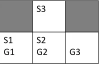
Figure 1: An instance that is solvable by the offline optimal solver, but cannot be solved by any online MAPF solver.
Consider first the question of what happens when an agent reaches its goal. One option is that when an agent reaches its goal it stays there. This results in a setting similar to the mentioned above lifelong MAPF (Ma et al. 2017). A differ-ent option is that an agdiffer-ent disappears when reaching its goal. Such an assumption makes sense when the goal is associated with some location that the agent can actually enter and stay there without interfering others, e.g., a private parking space. Orthogonal to the decision of what happens to an agent when it reaches the goal is the decision of what happens when a new agent appears. One option is to assume that a new agent immediately appears in its initial location. This can cause unavoidable collisions, as another agent may al-ready be in that location when the new agent appears. A dif-ferent assumption regarding new agents is that when a new agent appears it needs to perform a move action in order to enter its start location, and it can also wait as long as it wishes before doing so. This assumption also corresponds to a private parking space scenario, where the agent can wait in it, e.g., if it sees that its initial location in the graph is al-ready occupied. We refer to this private place as the agent’s
garage.
Consider the assumption that an agent disappears at its goal and the assumption that the agent appears in its garage. These correspond to a scenario where there is a private part of the world that is not managed in a centralized way, and the agents start from and wish to go to such private locations. To do so, the agents must pass through a public area that is controlled by some autonomous agent, e.g., an autonomous driving scenario where only the traffic in the city centers is fully automatized (Dresner and Stone 2008).
Next, we analyze the online MAPF problem under each of these four combinations of assumptions – staying at the goal or disappearing and appearing in the grid or in the garage.
Problem Analysis
S3
S1 G1
S2
G2 G3
S1 G2 S2
G2’ S2’ G1
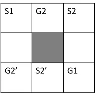
Figure 2: An instance in which no online MAPF solver can return the optimal solution.
Appears Stay at goal Disappear
In grid Collisions Collisions & Incomplete
(Obs. 1)
In garage Incomplete Complete (Prop. 2) (Obs. 1)
Table 1: Summary of theoretical results for online MAPF
Observation 1. If agents do not disappear when they reach their goals, then there are problem instances that are solv-able by an offline optimal solver but cannot be solved by any complete online MAPF solver.
Proof. Consider an online MAPF problem with 3 agents, situated in the grid given in Figure 1.S1,S2, andS3are the start locations of agents 1, 2, and 3, respectively. Similarly,
G1,G2, andG3are the agents’ goal locations. Now, assume that agent 1 appears first, then agent 2, and finally agent 3. An offline optimal solver will have agent 2 wait in its private space until agent 3 appears and reaches its goal. By contrast, any complete online MAPF solver will have to eventually decide to move agent 2 to its goal. We can construct an on-line MAPF problem that will have agent 3 appear only after this has occurred. When this occurs, the problem becomes unsolvable, as agent 3 can only reach its goal if agent 2 has not entered its starting location.
Proposition 2. An online MAPF problem where agents dis-appear at the goal and where new agents may wait before entering their initial location is solvable iff the offline part of the problem is solvable, assuming there exists a path for each agent from its initial location to its goal location.
Proof. If the offline part is solvable, we can then just let the new agents wait in their garages until all of the other agents disappear. The problem is then reduced to single agent short-est path. The other implication is trivial.
Since assuming that an agent appears immediately on the grid may cause unavoidable collisions, and assuming that the agent stays at the goal may lead to instances that no on-line solver can solve (Observation 1), we decided to focus the rest of this paper on online MAPF where the new agents appear in their garage and agents that reach their goal disap-pear. Note that waiting in a garage to enter the graph counts
as an action in the plan. Table 1 summarizes our observa-tions for the four combination of assumpobserva-tions.
Objective Functions
Now we ask the question of how to evaluate a solution
Π for an online MAPF problem. Porting the sum of costs measure from offline MAPF to online MAPF is straightfor-ward: the sum of costs of an online MAPF solution Π =
hπ0, π1, . . . , πmiis defined as the sum of costs of the
ex-ecuted plan Ex[Π], i.e.,f1(Π) = Pi∈A|Ex[Π]i|, where |Ex[Π]i|is the number of steps theithagents took until it
reached its goal.
Porting the makespan measure, however, is problematic, since makespan is defined as the arrival time of the last agent to its goal position. Due to the online nature of on-line MAPF, agents may keep emerging infinitely, resulting in Makespan= ∞, which is clearly undesirable. We now propose several possible objective functions intended to fill this gap. Let A be the set of agents, NotAtGoal(t) be the number of agents that are not at their goals at time steptyet, andoi be the length of the optimal (shortest) path for the
ithagent when no other agent is present. For a planΠand its executionEx[Π],|Ex[π]i|is the number of steps theith
agent took until it reached its goal. • Sum of agents not at goal over time.
f2(Π) =
∞
X
t=1
NotAtGoal(t)
• Sum of times over individual cost.
f3(Π) =
X
i∈A
|Ex[Π]i| −oi
Definition 3 (Objective Function Equivalence). A pair of objective functionsfxandfyare equivalent if for every on-line MAPF problem and every pair of solutionsΠandΠ0for that problem, we have
fx(Π)≤fx(Π0)⇔fy(Π)≤fy(Π0)
Proposition 4. All the objective functions listed above are equivalent to the sum of costs.
Proof. “f1 ⇔ f2” Letχti be 1 if the ith agent is not yet
at its goal location at time t, otherwise 0. Thenf1(Π) =
P i∈A
P∞ t=1χ
t
i andf2(Π) = P∞t=1
P i∈Aχ
t
i. Hence, by
swapping the sums,f1(Π) =f2(Π)for arbitraryΠ.
“f1 ⇔ f3” Since f1(Π) = Pi∈A|Ex[Π]i| = P
i∈A|Ex[Π]i|−oi+ P
i∈Aoi=f3(Π)+ P
i∈Aoi, and
be-causeP
i∈Aoi is a constant depending just on the problem
and not on the solution, it holds thatf1(Πx) ≤f1(Πy)⇔
f3(Πx)≤f3(Πy)for arbitrary plansΠx,Πy.
Thus, we only discuss the sum of costs objective function (f1) for online MAPF, and refer to a solution as optimal if it
minimizes the sum of costs.
Proof. Consider an online MAPF problem with 2 agents, situated in the grid given in Figure 2.S1 and G1 are the start and goal of agent 1, which is the first agent to appear. The agent has two shortest paths to reach its goal: going right and then down, or going down and then right. After the agent chooses one of these options, the second agent appears, ei-ther in S2 or in S2’. An offline optimal solver will know upfront where the second agent will appear and choose ap-propriately if the first agent will go down and right (avoid-ing S2) or right and down (avoid(avoid-ing S2’). An online MAPF solver cannot know this in advance and is thus bound to yield a suboptimal solution.
Online MAPF Algorithms
While Observation 5 states that guaranteeing an optimal so-lution is not possible with a complete solver, there is still a need to solve online MAPF problems in some principled way. In this section, we propose several online MAPF algo-rithms and discuss their properties.
The offline part of the problem, i.e., planning for the ini-tial set of agents, can be done by a different algorithm than the one used for the online part. We focus our discussion on the online part and assume that all algorithms we propose start with an optimal solution to the initial offline problem. Hence, in what follows we only describe only the replan
function, which is called when new agents appears. The in-put to such a replan functions is always the set of current agentsA, the set of new agentsA+, and the ongoing plan
πA, which is the plan the agents inAare currently
follow-ing. Note that more than one new agent may appear at the same time, and thusA+may contain multiple agents.
Replan Single and Replan Single Grouped
The first two algorithms we describe serve as a baseline. The Replan Single (RS) algorithm searches for an opti-mal path for each new agent, one at a time, while avoid-ing all other (already planned) agents. The Replan Savoid-ingle Grouped (RSG) algorithm searches for optimal paths for all new agents at once.
To formally describe RS and RSG, we introduce the fol-lowing helping notation. LetψπB
A be an optimal plan for a
group of agentsAwhile avoiding some planπBfor a group
of agentsB. This assumes that the groupsAandBare dis-joint. In particular,ψ∅Ameans an optimal plan for the agents in groupAwithout considering any agent that is not inA. Algorithms 1 and 2 list the pseudo codes for RS and RSG using our helping notationψAappropriately. Note that when
only one new agent appears, RS and RSG behave in the same way.
Algorithm 1Replan Single
functionRS(agentsA, new agentsA+, ongoing planπA) for eacha∈A+do
π←πA∪ψπaA
A←A∪ {a} end for
end function
Algorithm 2Replan Single Grouped
functionRS(agentsA, new agentsA+, ongoing planπ
A)
π←πA∪ψπAA+ A←A∪A+
end function
Analysis.RS can be solved in polynomial time, since it runs one single-agent path finding search. Therefore, in our im-plementation of the rest of the algorithms described in this work, we first run RS to obtain a baseline solution, and then try to improve on it in the rest of the runtime.
RSG, on the other hand, may require more runtime, de-pending on the number of new agents.
However, what can be said about the solution quality? Since both RS and RSG do not allow changing the plans of the other agents, then using them may lead to solutions of poor quality. Next, we propose a solution quality criteria that online MAPF algorithms can aim for in an effort to achieve better overall solution quality.
Snapshot Optimality
Definition 6(Snapshot Optimal). Asnapshot optimalplan in an online MAPF setting is a plan for all agents to their goal that is optimal in terms of sum of costs assuming no new agent will appear in the future.
There is no guarantee that always returning a snapshot optimal solution will result in an minimal sum of cost solu-tion for the online MAPF problem. In fact, we know from Observation 5 that such minimality guarantee is not possi-ble in online MAPF. Nonetheless, demanding that an online MAPF algorithm will return snapshot optimal solutions may bias it towards an overall low sum of cost in practice. Indeed, we observe this in our experimental results. Thus, we now propose several algorithms that provide such a guarantee.
Replan All The simplest way, conceptually, to return snapshot optimal solutions is to plan optimally forallagents from their current positions whenever new agent appears. We call this algorithm Replan All (RA), and list its (simple) pseudocode in Alg. 3.
Algorithm 3Replan All
functionRA(agentsA, new agentsA+, ongoing planπ
A)
A←A∪A+ π←ψ∅A
end function
RA is the extreme opposite of RS: it solves a much harder problem – offline MAPF for all current agents without con-sidering the already computed ongoing plan (πA) – but is
expected to return a high quality solution, i.e., a plan with a small sum of costs, since it computes the optimal solution for all of the agents currently present and the new agents.
Online Independence Detection
following. This can be wasteful in terms of runtime. More-over, changing the route of an agent that is already moving, which we refer to asre-routing the agent, may be undesir-able, as it requires communication with that agent and mod-ifying the agent’s plan may incur some overhead.
Next, we propose an algorithm that returns snapshot op-timal solutions but also attempts to minimize the number of re-routes. We call this algorithm Online Independence Detec-tion (OID) for online MAPF, since it is based on Standley’s Independence Detection (ID) algorithm (Standley 2010). The main idea of Standley’s ID is to plan for each agent separately while ignoring the other agents. If there is a conflict between the generated plans then the conflicting agents are merged into a group and replanned together. This process continues iteratively until there are no conflicts anymore.
The main idea of OID is very similar: allow the new agents to plan while ignoring the other agents. If there is a conflict with the plan of an already planned agent, then we merge the groups of conflicting agents and plan for them altogether (again disregarding the other agents). This is iter-ated until there are no conflicts anymore.
This adaptation of ID to online MAPF, however, may re-turn plans that are not snapshot optimal. The reason is that an online MAPF algorithm is called multiple times, whenever new agents appear. Consequently, when a new agenti1
con-flicts with an already existing agenti2, it is not sufficient to
replan fori1andi2together sincei2may have been grouped
with other agent, e.g.,i3in the previous call. There, perhaps
agenti3chose a longer path in the previous call to allowi2
use a shorter path. Now, wheni2is replanning due to a
con-flict with the new agenti1, perhaps it frees up locations that
i3can use to have a shorter path for itself.
To correct this, we modify OID so that it keeps track of the groups used to create the incumbent plan. Algorithm 4 lists the pseudo code for OID. First, the algorithm requires that the set of already planned agentsAconsists of mutually dis-joint and collectively exhaustive sets of agentsg1, g2, ..., gm,
and the ongoing planπgi for everygi, such that πgi is the
lowest cost plan for the agents ingi. When new agentsA+
appear, each of them is placed into a new group and an opti-mal plan for each group is found, disregarding all the other agents (lines 2–6). Then the algorithm iteratively resolves the conflicts until there are no more conflicting groups. As-sume there is a conflict of plans between groupsgi andgj.
Then the algorithm tries to find such a plan forgithat avoids
conflicts with the agents from groupgjwhile not
deteriorat-ing the plan in terms of the sum of costs (line 13). If it does not succeed, it tries analogically to replan forgjwhile
avoid-inggi(line 15). If it still did not succeed, it merges the
con-flicting sets of agents and replans for them together, while, again, disregarding all other agents (lines 17–20). However, this way the algorithm could get stuck in an infinite loop, that is why it is necessary to first check whether the two conflicting groups were already in conflict together before, and thus merge and replan them straight away (lines 9–12).
Theorem 7. OID returns a snapshot optimal solution if it is given a disjoint partition of agents to groups g1, . . . gm such that for every groupgithe cost of its current planπgi
is equal to the cost ofψ∅gi.
Algorithm 4Online Independence Detection
1: function OID(agents A = ˙Sm
i=1gi, new agents A+,
ongoing planπA)
Require: πgifor each groupgi
2: k←m+ 1
3: for eacha∈A+do
4: gk←a
5: πgk←ψ
∅
a
6: k←k+ 1
7: end for
8: whilegiandgjconflictdo
9: ifgi, gjconflicted beforethen
10: gi←gi∪gj
11: gj← ∅
12: πgi ←ψ
∅
gi
13: else ifψgπigj is as good asπgithen
14: πgi ←ψ
πgj gi
15: else ifψπgi
gj is as good asπgj then
16: πgj ←ψ
πgi gj
17: else
18: gi←gi∪gj
19: gj← ∅
20: πgi ←ψ
∅
gi
21: end if
22: end while
23: end function
Proof outline. Consider the output of OID after being called by a replan function. OID outputs a new partition of agents to groupsg01, . . . g0m0 that includes the new agents
along with a plan to each of these groups. Since OID never breaks a group, then every group in the original set of groups
g1, . . . gm must be equal to or a subset of one of the new
groups g01, . . . gm0 0. Since OID returns an optimal plan for
each of the new groups, then it cannot miss an optimal plan for any agent.
Corollary 8. If the ongoing plan was snapshot optimal and OID is used to replan when new agents appear then OID is guaranteed to always return snapshot optimal solutions.
Corollary 8 follows by induction due to Theorem 7 and the fact the initial plan is snapshot optimal. Since OID at-tempts to minimize the number of existing agents it replans for, it has the potential to save runtime and require fewer re-routes than RA.
Suboptimal Independence Detection
As noted earlier, returning a snapshot optimal plan does not guarantee an optimal solution to the online MAPF problem. Therefore, we propose to change OID by allowing it to re-turn plans whose sum of costs is at mostDtimes more than the optimal sum of costs but allowing it to further reduce the number of agents that have to deviate from the ongoing plan. We call this algorithm Suboptimal OID (SubID).
In details, when OID replans for the group of agents gi
while avoidinggjand ignoring all other agents (line 13 and
symmetrically line 15), it only accepts plans that have ex-actly the same sum of costs as that of the optimal plan forgi
while ignoring all other agents (the sum of costs value be-ingf1(ψ
πgj
gi )). It is likely that such a solution does not exist.
SubID allows the new plans to have higher cost, namely any cost in the range[f1(ψ
πgj
gi ), D·f1(ψ
πgj
gi )]. This is expected
to increase the likelihood that such a plan will be found.
Theorem 9. Given a disjoint partition of agents to groups
g1, . . . gmsuch that for every groupgithe cost of its current planπgiis at mostw1times the cost ofψ
∅
gi, then SubID with
parameterD = w2 will return a solution whose cost is at
mostw1·w2.
Proof outlineThe proof is similar to that of Theorem 7: every groupgiis a contained in exactly one group from the
solution of SubID. The added suboptimality is a factor of at mostw2and the suboptimality of the existing plan is at most
w1thus the overall suboptimality isw1·w2.
A direct corollary of Theorem 9 is that if SubID is always used to replan when new agents appear then after them re-plan calls SubID will output a re-plan whose cost is at most
Dmtimes the cost of a snapshot optimal plan.
Results of Experiments
We implemented all the algorithms and evaluated their performance on a set of randomly generated problems. All experiments were conducted on Dell PC with an IntelR CoreTM i7-2600K processor running at 3.40 GHz with 8 GB of RAM.
Instances
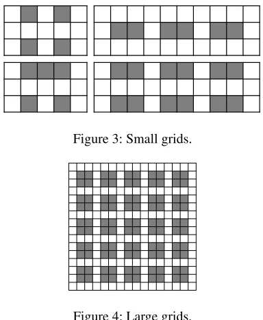
We created two datasets of online MAPF problems based on 4-connected grids designed to simulate intersections for au-tonomous vehicles. The first dataset is on small and dense grids, chosen from the 4 types of small grids depicted in Figure 3. Each problem started with no agents present at the outset. Then we are adding new agents, the total num-ber of which is in the range{10, 12, 15, 17, 20, 22, 25}. The starting time of each agent is set uniformly at random from the interval[1,30], so a number of agents may appear at the same time. The start location is a random location from a randomly picked margin of the map and the goal is randomly picked from the opposite margin. We generated 5 problems for each configuration. Altogether this dataset contained 140 problems.
The second dataset is on a larger grid depicted in Figure 4. The starting time of each agent is set uniformly at ran-dom from the interval [1,100]. The number of new agents
Figure 3: Small grids.
Figure 4: Large grids.
to appear over these timesteps increments from 60 to 70. The agents are moving from a randomly picked margin to another randomly picked margin. No agent is present at the outset. We generated 5 problems for each configuration. Al-together we generated 30 testing instances.
Implementation Details
All the proposed algorithms require an optimal offline MAPF solver, adapted to our assumptions that a new agent appears in its garage and agents disappear at their goals. We created two such modified optimal offline MAPF solvers: one based on a reduction to Boolean satisfiability (SAT) via the Picat language and compiler (version 2.2#3) (Bart´ak et al. 2017), and the other based on the Conflict-Based Search (CBS) algorithm (Sharon et al. 2015). For the first dataset (small grids) we used the Picat-based solver and for the sec-ond dataset (large grid) we used the CBS-based solver. This is because Picat-based solvers perform better on small and dense grids and CBS-based solver performs better on large grids (Bart´ak et al. 2017).
Dataset #1: Small Grids
We ran the following algorithms on the small grids dataset: Replan Single (RS), Replan Single Grouped (RSG), Replan All (RA), Online Independence Detection (OID), and Sub-optimal ID (SubID) withDchosen to be 1.1. For every in-stance, we always run first RS and then the algorithm in question. Whenever the runtime for a newly appeared agent exceeds the given time limit, which was set to 30 seconds, the output from RS is taken into results. The reason is that RS is done extremely quickly and it is always good to have some solution rather than no solution. The number of in-stances, where the timelimit was reached and thus the result from RS was taken, can be seen in Table 2.
#agents RSG SubID OID RA 10 0.00 1.70 1.70 0.55 12 0.00 2.55 2.20 1.05 15 0.05 5.90 4.25 2.40 17 0.35 6.55 7.10 3.40 20 1.20 9.55 9.80 5.65 22 1.70 10.85 10.55 9.40 25 3.50 11.65 11.65 10.00
Table 2: The average number of timeouts per instance of each algorithm.
as the number ofchanges) is shown in Table 3. The number of changes for RS and RSG is always zero, since it never replans for the other agents, so we do not report it in Table 3. The results clearly show that OID requires fewer changes than RA, and SubID requires even fewer changes than OID. For example, with 15 agents, SubID required on average 1.5 changes, while OID required 3.45 and RA 6.45. The slight decrease in the number of changes for 20 agents is caused by the increase in the number of timeouts and therefore more RS calculations that avoid changes is used.
The relative gain in terms of the sum of costs over RS is shown in Table 4. The expectations that RA will always be the best w.r.t. the sum of costs have been confirmed. It is worth noticing that SubID, which does not return an optimal solution in every replan, brings more or less the same gains in terms of the sum of costs as OID. Thus, SubID shows promising results, with comparable sum of costs to OID but significantly fewer changes.
#agents SubID OID RA
10 2.65 3.30 5.15
12 2.05 2.80 3.80
15 1.50 3.45 6.45
17 3.80 3.85 10.05 20 2.85 2.65 10.15
22 2.95 4.25 6.80
25 1.90 2.55 6.40
Table 3: Avg. # of re-routes for smaller grids using Picat.
#agents RSG SubID OID RA 10 1.01 1.06 1.06 1.10 12 1.02 1.08 1.09 1.14 15 1.03 1.04 1.11 1.17 17 1.05 1.14 1.13 1.22 20 1.04 1.04 1.04 1.19 22 1.06 1.06 1.10 1.15 25 1.05 1.07 1.08 1.15
Table 4: Avg. gain in SOC over RS for smaller grids using Picat.
Dataset #2: Large Grids
The experiments on large grids dataset were carried out in the same way. The number of instances where time limit
#agents RSG SubID OID RA 60 0.0 1.0 0.4 0.8 62 0.0 0.0 0.2 0.6 64 0.0 1.0 0.8 0.4 66 0.0 0.0 0.2 0.6 68 0.0 0.0 0.0 0.4 70 0.0 0.6 1.0 0.4
Table 5: Avg. # of timeouts on the larger grid using CBS.
#agents SubID OID RA
60 5.6 13.4 30.0
62 4.6 11.4 26.0
64 4.4 11.6 25.0
66 5.0 16.6 32.0
68 6.4 12.4 27.4
70 5.8 12.0 24.6
Table 6: Avg. number of re-routes for larger grid using CBS.
was reached is shown in Table 5. The number of changes is shown in Table 6, and the relative gain w.r.t. the sum of costs is shown in Table 7. Briefly speaking, the results are in concordance with those of small grids.
While here again we see a clear advantage in terms of the sum of costs for RA, OID, and SubID compared to RS, the differences are significantly smaller. This is because larger grids are sparser, and thus it is easier for RS to find a higher quality solution. The differences in the sum of costs between RA, OID, and SubID are negligible, but SubID still shows a significant advantage in terms of the number of changes. For example, with 66 agents SubID required on average only 5 changes while RA required 32, and their sum of costs was virtually the same.
In conclusion, SubID confirms to have brought the best trade-off between the quality of the resulting plans and the computational efficiency.
Related Work
The termonline planningin general refers to planning that is done while executing a plan, in contrast tooffline plan-ningwhere all the planning is done upfront. Many papers on online planning defer planning to execution to minimize the computational effort of creating a complete plan for every contingency offline. This includes the seminal work of Korf on Real-Time A* and its many successors (Korf 1990). This is different from our setting, where some of the planning is
#agents RSG SubID OID RA 60 0.997 1.008 1.015 1.015 62 0.994 1.008 1.012 1.012 64 1.000 1.009 1.012 1.013 66 1.000 1.008 1.009 1.009 68 0.996 1.007 1.009 1.009 70 0.998 1.009 1.010 1.011
done online because the agents do not know in advance how many and where the new agents will appear.
Online MAPF can be viewed as an instance of ad-hoc teamwork(Stone et al. 2010), which exactly addresses cases where the agents constantly need to coordinate with new agents. However, the form of interactions between the agents in online MAPF is very specific – they cannot collide with each other, while ad-hoc teamwork usually involves deeper forms of collaboration. In the motion planning literature, there is work on single robot online planning that replans for newly observed obstacles by using pre-defined planning patterns (Majumdar and Tedrake 2013). In addition, some prior work on multi-robot motion planning that are funda-mentally forms of prioritized planning (Van Den Berg and Overmars 2005) can be adapted to the online case, resulting in a behavior similar to RS. Other motion planning tech-niques (Dobson et al. 2017; Godoy et al. 2015) are designed for offline, continuous spaces and adapting them to a discrete and online MAPF is non-trivial.
Conclusion and Future Work
In this paper, we study theonlineversion of the multi-agent pathfinding problem, in which new agents appear during ex-ecution of a plan. We analyzed several variants of the prob-lem theoretically, showing which of these variants can be solved by an online MAPF algorithm. Then, we proposed several online MAPF algorithms. The pros and cons of each algorithm are analyzed and demonstrated experimentally. While the baseline replan single algorithm is the fastest, its solution quality is, in some configurations, poor compared to the replan all baseline. OID and SubID provide further improvements to replan all, as they minimize the sum of costs while also aiming to force fewer agents to change their planned paths. Future work we expand on this is modifying the replanning process to try to find individual plans that are close to the ongoing plan (Felner et al. 2007) and/or plans that minimize the probability of conflicts in the future.
Acknowledgement
This research is supported by the Czech-Israeli Coopera-tive Scientific Research Project 8G15027, by SVV project number 260 453, by the EU and the Ministry of Industry and Trade of the Czech Republic under the Project OP PIK CZ.01.1.02/0.0/0.0/15 019/0004688, and by ISF grant no. 210/17 to Roni Stern. Roman Bart´ak is supported by the Czech Science Foundation project 18-07252S.
References
Bart´ak, R.; Zhou, N.-F.; Stern, R.; Boyarski, E.; and Surynek, P. 2017. Modeling and solving the multi-agent pathfinding problem in picat. InInternational Conference on Tools with Artificial Intelligence (ICTAI), 959–966.
Dobson, A.; Solovey, K.; Shome, R.; Halperin, D.; and Bekris, K. E. 2017. Scalable asymptotically-optimal multi-robot motion planning. InInternational Symposium on Multi-Robot and Multi-Agent Systems (MRS), 120–127. IEEE.
Dresner, K. M., and Stone, P. 2008. A multiagent approach to autonomous intersection management. J. Artif. Intell. Res.
31:591–656.
Erdem, E.; Kisa, D. G.; ¨Oztok, U.; and Sch¨uller, P. 2013. A general formal framework for pathfinding problems with multiple agents. InAAAI.
Felner, A.; Stern, R.; Rosenschein, J. S.; and Pomeransky, A. 2007. Searching for close alternative plans. Autonomous Agents and Multi-Agent Systems14(3):211–237.
Felner, A.; Stern, R.; Shimony, S. E.; Boyarski, E.; Gold-enberg, M.; Sharon, G.; Sturtevant, N. R.; Wagner, G.; and Surynek, P. 2017. Search-based optimal solvers for the multi-agent pathfinding problem: Summary and challenges. In In-ternational Symposium on Combinatorial Search (SoCS), 29– 37.
Godoy, J. E.; Karamouzas, I.; Guy, S. J.; and Gini, M. 2015. Adaptive learning for multi-agent navigation. In the Inter-national Conference on Autonomous Agents and Multiagent Systems (AAMAS), 1577–1585.
Korf, R. E. 1990. Real-time heuristic search. Artif. Intell.
42(2-3):189–211.
Ma, H.; Li, J.; Kumar, T.; and Koenig, S. 2017. Lifelong multi-agent path finding for online pickup and delivery tasks. InProceedings of the 16th Conference on Autonomous Agents and MultiAgent Systems, 837–845. International Foundation for Autonomous Agents and Multiagent Systems.
Majumdar, A., and Tedrake, R. 2013. Robust online motion planning with regions of finite time invariance. InAlgorithmic Foundations of Robotics X. Springer. 543–558.
Pallottino, L.; Scordio, V. G.; Bicchi, A.; and Frazzoli, E. 2007. Decentralized cooperative policy for conflict resolu-tion in multivehicle systems. IEEE Transactions on Robotics
23(6):1170–1183.
Sharon, G.; Stern, R.; Felner, A.; and Sturtevant, N. R. 2015. Conflict-based search for optimal multi-agent pathfinding.
Artificial Intelligence219:40–66.
Silver, D. 2005. Cooperative pathfinding. InArtificial Intel-ligence and Interactive Digital Entertainment (AIIDE), 117– 122.
Standley, T. S. 2010. Finding optimal solutions to coopera-tive pathfinding problems. InAAAI Conference on Artificial Intelligence.
Stone, P.; Kaminka, G. A.; Kraus, S.; Rosenschein, J. S.; et al. 2010. Ad hoc autonomous agent teams: Collaboration with-out pre-coordination. InAAAI.
Surynek, P.; Felner, A.; Stern, R.; and Boyarski, E. 2016. Effi-cient SAT approach to multi-agent path finding under the sum of costs objective. Inthe European Conference on Artificial Intelligence (ECAI), 810–818.
Van Den Berg, J. P., and Overmars, M. H. 2005. Prioritized motion planning for multiple robots. InIEEE/RSJ Interna-tional Conference on Intelligent Robots and Systems (IROS), 430–435.