DOI: 10.9781/ijimai.2018.09.001
* Corresponding author.
E-mail address: [email protected]
I. Introduction
R
ECENTLY, image processing has several applications in different areas such as; industry agriculture, medicine, etc. Image segmentation is considered the most important step in image processing [1]. This process is classifying the pixel in the image depending on its intensity value. In literature, different methods have been proposed for image segmentation, including edge based method [2] neural network based method [3],watershed based method [4], clustering based method[5], and artificial threshold based method [6].
Thresholding method is a simple and effective tool to isolate objects of interest from the background. Its applications include several classics such as document image analysis, whose goal is to extract printed characters [7] logos, graphical content, or musical scores; also it is used for map processing which aims to locate lines, legends, and characters [8]. It is also used for scene processing, aiming for object detection and marking [9];; Similarly, it has been employed to quality inspection for materials discarding defective parts[10].
Thresholding techniques are used for segmenting the image into two (bi-level) or more classes (RGB). The binary level thresholding is taking only one threshold value (t) and then testing every pixel with specific intensity value, if it is higher, the threshold value (t) classified as the first class and the other pixel with a different intensity value are classified as second class. In multilevel thresholding, the pixels
in the image are divided into more than one class, where, every class is taken a specific threshold value [11-13]. Basically, two approaches called parametric and nonparametric can be used to determine the optimal threshold value [12]. In parametric approach, some parameters of a probability density function should be estimated for classifying the classes of image. But this approach is computationally expensive and time consuming whereas that non parametric approach optimizes several criteria such as; the error rate, the entropy, etc, in order to determine the optimal threshold values However, there are two methods can be used for binary level thresholding; Otsu’s and Kapur. Otsu method uses the maximization of between classes variance [14].
Kapur method maximizes the entropy to measure the homogeneity of the classes [15]. The computational complexity of the two methods for multilevel thresholding is increasing for each new threshold [16].
Many optimization techniques deal with multilevel thresholding (MT) for image segmentation such as; Particle Swarm Optimization (PSO) [17] , Moth Flame Optimization (MFO) [18], Genetic Algorithm (GA) [19], Whale Optimization Algorithm (WOA) [18], Ant Colony Optimization (ACO) [20].
Recently, EMO contributed to solving many engineering problems such as; control systems [22], array pattern optimization in circuits [23],neural network training [24], vehicle routing [25], communications [26], flow-shop scheduling [27], image processing [28] Although EMO algorithm is consistent with characteristics of other approaches, EMO’s performance generates a better precision and computation time in most of the studied cases when it is compared with other metaheuristic optimization techniques such as; Cuckoo Search (CS), Sine Cosine algorithm (SCA) and MFO, and WOA. However, EMO
Keywords
Image Segmentation, Multilevel Thresholding, Otsu’s Entropy,Electromagnetic Optimization, Levy Function.
Abstract
Image segmentation is considered one of the most important tasks in image processing, which has several applications in different areas such as; industry agriculture, medicine, etc. In this paper, we develop the electromagnetic optimization (EMO) algorithm based on levy function, EMO-levy, to enhance the EMO performance for determining the optimal multi-level thresholding of image segmentation. In general, EMO simulates the mechanism of attraction and repulsion between charges to develop the individuals of a population. EMO takes random samples from search space within the histogram of image, where, each sample represents each particle in EMO. The quality of each particle is assessed based on Otsu’s or Kapur objective function value. The solutions are updated using EMO operators until determine the optimal objective functions. Finally, this approach produces segmented images with optimal values for the threshold and a few number of iterations. The proposed technique is validated using different standard test images. Experimental results prove the effectiveness and superiority of the proposed algorithm for image segmentation compared with well-known optimization methods.
Multilevel Thresholding for Image Segmentation
Using an Improved Electromagnetism Optimization
Algorithm
Ashraf M. Hemeida
1*, Radwa Mansour
2, M. E. Hussein
21
Electrical Engineering Department, Faculty of Energy Engineering, Aswan University (Egypt)
2
Computer Science Division, Department of Mathematics Faculty of Science, Aswan University (Egypt)
algorithm simulates the mechanism of attraction-repulsion which subject to the electromagnetic law of physics to develop the individuals of population based on their objective function values [21]. The main idea of EMO is to move a particle through the space following the force exerted by the rest of the population. Using the charge of each particle depending on its objective function value, the force is calculated.
This paper proposes an improved EMO algorithm based on levy function (EMO-levy) for multilevel thresholding of image segmentation. Different standard images are used to validate the proposed technique compared with other well-known optimization techniques such as; original EMO, CS, SCA, MFO and WOA. The developed approach produces a multilevel segmentation of digital images with few number of iterations and fast computational time.
The organization of the paper is as follows. In Section II, presents the developed Electromagnetism Optimization Algorithm with levy function (EMO.levy). Section III illustrates the problem definition of multilevel thresholding (MT) and the application of developed optimization algorithm for solving it. Section IV presents comprehensive results obtained by the developed algorithm, comparing with other techniques. Section V provides the outstanding features of the proposed algorithm. Finally, Section VI gives the final conclusions of the paper.
II. Improved Electromagnetism Optimization Algorithm
A. EMO
The EMO formulation has been developed to find a global solution of a nonlinear optimization problem with satisfying the operating constraints as [12]:
1 2 3
max ( ),
f x x
=
( , , ,.. )
x x x x
k∈
Z
(1)
Subject to
where, f: Z→Z is a nonlinear function,
, is the lower limit and is the upper limit.
EMO technique uses some variable such as: m → number of population inside one iteration
n → dimensional control variable xj,t and t refers to the iteration number of the algorithm.
Et=(E1,t,E2,t,E3,t,…………Em,t) →is the initial population in the same iteration t which is taken by random samples from search space X of image histogram. After the initialization of Et, EMO continues its iterative process until reaching to the maximum number of iterations
[30].
B. Lévy Electromagnetism Optimization Algorithm (EMO.levy)
Lévy flight distribution is integrated in EMO technique to enhance the searching capability and exploration ability of this optimization algorithm by increasing its probability of producing new solutions to avoid stagnation of algorithm and to avoid trapping in local minima. Levy flight is a random process for generating a new solution based on random walk where its steps are captured from a Lévy distribution. The new population position that is based on Lévy distribution can be found as follows [35]:
( )
new
i i
X = X + ∝ ⊕Levy
β
(2)
where, represents a random step size parameter. is the entry wise multiplication and is a Lévy Flight distribution parameter. The step size can be found as:
( )
~ 0.01 1/(
t t)
i best uLevy X X
v β
β
∝ ⊕ −
(3)
where, u and v are normally variables produced by normal distribution where,
( )
2~ 0,
uu N
φ
,
~ 0,
( )
2v
v N
φ
(4)
(
)
(
)
(
)
[
]
1/
1 sin / 2
, 1
1 / 2
u v
β
β
π β
φ
φ
β
β
Γ + × ×
= =
Γ + ×
(5)
where , is the standard gamma function and, . To enhance the exploitation of EMO the best search agent is updated by using variable bandwidth as follows:
5
new t
best best w
X = X ±C ×K
(6)
where, is a random number in [0, 1]. is a variable bandwidth that decreases dynamically as:
( )
max
s t w
K
=
K e
×(7)
min max max ln K K s T =
(8)
where, and are the maximum and the minimum limits. is the current iteration and is the maximum number of iterations. However, the solution process of EMO technique is going through basic steps:
Step1- Input variable itermax, iterlocal, α local search parameter, m
number of population, n dimensional of x.
Step2- The algorithm in this step makes initialization by taking
random particles from the search space between lower and upper bound at same iteration=1 ,then the objective function values
f (xi,t) are calculated over all population Ei,t, (where i=1,….,m) from the results, the best value of Ei,t is Eb that represents the optimum
objective function value f(xi,t) which is generated from the best point .
where,
,
( )
,i t i t
E
=
f x
(9)
,
arg max ( )
b
t i t
x = f x
(10)
( )
b b
t t
E = f x
(11)
Step3- The force value must be calculated for each individual of the
population in Et, It is known that each individual of the population has a value of objective function f(xi,t) therefore a value the electromagnetic charge (qi,t) can be calculated based on the value of its function as:
1 , , , exp m i b
i t t
i t
b
i t t
E E q n E E = − = − −
∑
(12)
(
)
( )
( )
(
)
( )
( )
, ,
, , 2 , ,
, , ,
, ,
, , 2 , ,
, ,
,
,
i t j t
i t j t i t j t
j t i t
t i j
i t j t
j t i t i t j t
j t i t
if f f
F
if f f
q
q
x
x
x
x
x
x
q
q
x
x
x
x
x
x
> = ≤•
−
−
•
−
−
(13)
The total force that affects the point xi,t can be calculated as:
, 1,
m T t i j j i j
F F
= ≠
=
∑
(14)
In this step, each point xi,t except xb is moving from its place to another using attraction or repulsion force depending on its charge which is based on objective function value of each other. Hence, the points which have strong charge with a better objective function value will be attracted to each other, and the point xi,t will move to point ai,t
(
)
, , , 1, 2, , .. t
i i t i t t
i
F
x x RNG i m i b
F
= + = … ≠
(15)
where, RNG → the range of movement toward the lower or upper bound.
l → the standard uniform distribution with minimum 0 and maximum 1.
Step4- In this step, the algorithm makes local search. After all points
are moved from its place except xb point on search space, the iteration
of local search (iterlocal) is generated and each point performs a local search for neighbor points of ai,t and generates its d neighbor points for selecting a better point di,t which generates a better objective function more than the current. Then, the local search process will be stopped when the iteration (iterlocal) is finished.
After all these steps, the algorithm goes to next iteration, while the point xi,t becomes either ai,t or di,t in next iteration (t+1).
III. Image Segmentation Using Improved Emo Method
The effective way for image segmentation is thresholding method. This method is used for classifying the binary level image and multilevel image based on the value of its intensity level (L). This process converts the image into (m×n) pixel. Each pixel carries an intensity level (L) value that can be classified to the class which it belongs.
If the image is grey level, the thresholding method classifies it into two classes R1, R2 with only a threshold value (th), hence, if the pixel has an intensity level value > th, it can be classified as the first class R1 and otherwise classified to second class R2.
1 0
R ← p if < <p th
2 1
R ← p if th p L< < −
(16)
For multilayer image, the image is divided into more than two classes, every class has a specific threshold value, Therefore for multilayer image TH=(th1,th2,th3,……….thL-1), the classes are (R1,R2,….RN).
where, N is the number of classes
1 1 0
R ← p if < <p th
1 2
R ← p if p th> 3 2
R ← p if p th>
…………..
1
N N
R ← p if p th> −
(17)
The problem for both bi-level and multilevel thresholding is to select the th values which correctly identify the classes. Otsu’s and Kapur’s methods are well-known approaches for determining such values. Both methods propose a different objective function which must be maximized in order to find optimal threshold values, just as it is discussed below.
A. Otsu’s Method
Otsu method is one of the methods used to segment the image by maximizing variance value among classes then calculating the value of objective function as:
2
( )
max(
r(th))
otsu b
f th
=
σ
(18)
where,
The optimization problem is decreased to get a better intensity level (threshold) that maximizes (18). The previous objective function is used for grey level image because it contains one threshold (th). However, equation (18) can be rewritten to be used in the case of RGB images as;
2
( ) max( (TH))r
otsu b
f TH = σ
(19)
where,
TH=( ) and k is number of class
2 1 r k B i r i
σ
σ
= =∑
(20)
2 ( )r r r r
i w mi i mt
σ
= −(21)
where,
i→ refers to a certain class, and k is number of classes
r→ refers to a constant number equal to 1 in grey level image (r=1,2,3 in RGB image)
→ refers to the variance among classes R (Otsu´s variance) →refers to the mean of a class
1
0
1 0
( )
1th r r i r i
iph
m
w th
==
∑
2 1 11 1
( )
2th r r i r i th
iph
m
w th
= +=
∑
…….
11 1
( )
k
r L
r i
k r
i th k
iph
m
w th
− = +=
∑
(22)
where,
w
1r→ refers to the probability of occurrence1
1
1
( )
r th ri i
w th
ph
=
=
∑
( )
21 2 1 th r r i i th
w th
ph
= +
=
∑
( )
1 1 k L r r k i i thw
−th
ph
= +
=
∑
(23)
where, that is the probability distribution of the intensity level values which can be calculated as:
1
, r
1, 2,3
r r i iin grey image
h
ph
in RGBimage
N
=
=
(24)
where, 11
N r i iph
==
∑
(25)
are histogram distribution values which indicate the number of pixels corresponding to the i intensity level, N is total number of pixel in the image.
Electromagnetism optimization is used to find the optimal decision variable which is considered in the segmentation problem as threshold (TH)[20] as:
Maximize Subject to
where, 0 < < 255 this is lower and upper bounded of threshold i=1,..,k and here k refers to different thresholds (TH).
B. Kapur Method
Another nonparametric method that is used to determine the optimal threshold values has been proposed by Kapur [15]. It is based on the entropy and the probability distribution of the image histogram. This method aims to find the optimal th which maximizes the overall entropy. The entropy of an image measures the compactness and separability among classes. In this sense when the optimal th value appropriately separates the classes, the entropy has the maximum value. For the bi-level example the objective function of the Kapur’s problem can be defined as:
( )
1 21,2,3
,
1
c c kapur
if RGB image
f th H H c
if greyimage
= + =
(26)
where, the entropies H1 and H2 are computed by the following model:
1
1
1 0 0
ln
th c c
C i i
c c i ph ph H w w = =
∑
,
2 1 1 1ln
c c
L
C i i
c c i th ph ph H w w = + =
∑
(27)
where, is the probability distribution of the intensity levels which is obtained using (24). w0c and
1
c
w are probabilities distributions for C1 and C2, respectively. Similar to the Otsu’s method, the entropy-based approach can be extended for multiple threshold values, for such a case it is necessary to divide the image into k classes using the similar number of thresholds. Under such conditions, the new objective function is defined as:
( )
{
1, 2, 3 11
,
kapur
k if RGB Image
c
f TH i
if grey Image i
H
c
= = =∑
(28)
where, 1 11 0 0
ln
th c c
C i i
c c i ph ph H w w = =
∑
2 1 21 1 1
ln
th c c
C i i
c c i th ph ph H w w = + =
∑
………
1 1 1
ln
k
c c
L
C i i
k c
i th k
c k ph ph H w w = + − − =
∑
(29)
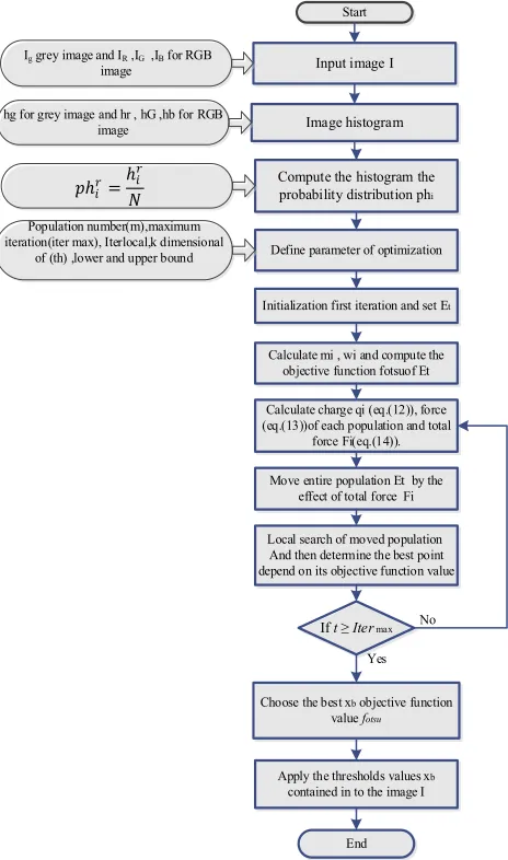
The solution process of image segmentation using the developed optimization algorithm can be shown in Fig. 1.
Input image I
Ig grey image and IR ,IG ,IB for RGB
image
Image histogram
hg for grey image and hr , hG ,hb for RGB image
Compute the histogram the probability distribution phi
Define parameter of optimization Population number(m),maximum
iteration(iter max), Iterlocal,k dimensional of (th) ,lower and upper bound
Initialization first iteration and set Et
Calculate mi , wi and compute the objective function fotsuof Et Calculate charge qi (eq.(12)), force (eq.(13))of each population and total
force Fi(eq.(14)). Move entire population Et by the
effect of total force Fi Local search of moved population
And then determine the best point depend on its objective function value
If t ≥ Iter max
Choose the best xb objective function
value fotsu
Apply the thresholds values xb
contained in to the image I End Start
No Yes
𝑝𝑝ℎ𝑖𝑖𝑟𝑟=ℎ𝑖𝑖 𝑟𝑟
𝑁𝑁
Fig. 1. Flowchart of the proposed method for image segmentation.
IV. Results and Discussion
In this section, different test images are used to validate the proposed EMO with levy algorithm
A. Standard Test Images
Fig. 2 indicates these test images and their histogram distributions which refer to the number of pixels in the images at each different intensity value found in these images.
The performance of proposed EMO with levy algorithm based multilevel thresholding is compared with some well-known optimization algorithms such as; CS [31, 32], MFO [18], WOA [18], SCA [33, 34]. All algorithms have been tested with the same condition of stop criterion;100 iterations and 25 population. At the end of each test, the Peak Signal-to-Noise Ratio (PSNR) is computed as:
10
255 20 log
PSNR
RMSE
=
(30)
The PSNR is an important value which measures the accuracy of a segment image comparing with the original image.
where, RMSE is the root mean square error, which can be calculated as:
( )
( )
(
0)
1 1
,
,
ro co
r r
th
i j
RMSE
ro co
I i j
I i j
= = =
×
−
∑∑
(31)
where, ro is the total number of rows of an image, co is the total
number of column of the image, r is depending on the type of image (RGB image r=1,2,3), refers to the segmented image, refers to the original image.
In each experiment the stop criteria is set to 100 iterations. In order to verify the stability at the end of each test the standard deviation (STD) is obtained (Eq. (32)). If the STD value increases the algorithms becomes more instable.
(
)
max
1 iter
i
i
STD
s m
Ru
=
=
∑
−
(32)
Table I indicates the parameters of EMO with Levy function (EMO.levy). The maximum number of iterations is taken as 100, this parameter represents the stop criterion of the optimization process. However, which the stop criterion is taken as the number of times in which the best fitness values remains without change. Iterlocal=100 is the number of times that the algorithm do local search with 25 population at every external iteration.
TABLE I. Parameters of Emo With Levy
Itermax Iterlocal d M(population)
100 10 0.025 25
(a)
0 50 100 150 200 250 300
0 0.002 0.004 0.006 0.008 0.01 0.012
(b)
(c)
0 50 100 150 200 250 300
0 0.002 0.004 0.006 0.008 0.01 0.012
(d)
(e)
0 50 100 150 200 250 300
0 0.005 0.01 0.015 0.02 0.025 0.03
(f)
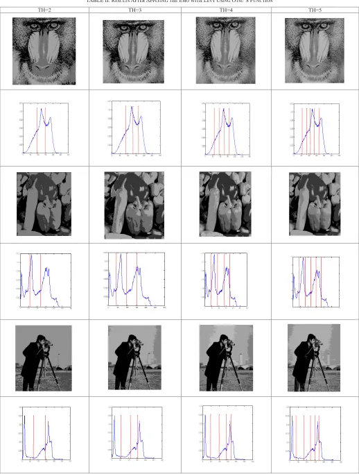
TABLE II. Results After Applying the Emo with Levy Using Otsu´S Function
TABLE III .The Best Fitness Value Obtained from all Algorithms for Test Image
Image K EMO.levy EMO CS SCA MFO WOA
Baboon 2 1552.5 1550.2 1552.5 1455.2 1538.81 1545.92
3 1644.7 1645 1645 1527.8 1592.98 1635.7
4 1699.4 1691 1699.5 1663.4 1647.93 1669.83
5 1725.6 1720 1725.8 1628.2 1705.93 1682.48
pepper 2 2858.5 2857.5 2861.1 2324.5 2435.5 2433.36
3 3059.9 3059.8 3059.9 2550.4 2574.7 2493.18
4 3145.7 3144.8 3145.7 2537.9 2647.67 2632.9
5 3189.8 3189.4 3189.7 2603.8 2669.47 2682.01
Cameraman 2 3646.6 3646.5 3643.6 3515.8 3643.31 3649.36
3 3721.8 3721 3718.7 3680.5 3720.25 3690.11
4 3778.2 3777.4 3774.5 3749.18 3748.75 3760.5
5 3809.4 3809.4 3805.7 3718.18 3758.72 3795.86
TABLE IV. The Best Threshold Values Obtained from All Algorithms for the Test Image
Image k EMO with levy EMO CS MFO WOA SCA
Baboon 2 97,149 93,147 97,149 111,133 83,151 103,150
3 86,126,162 85,124,160 84,123,160 74,137,168 27,83,144 81,112,145
4 71,105,136,167 60,96,127,161 71,106,137,168 44,84,133,173 96,109,134,152 61,82,128,164
5 64,95,121,146,173 54, 83,107,137,168 68,100,125,149,174 46,94,158,189,219 32,77,101,148,207 75,99,140,159,188
pepper 2 82,143 56,120 49,116 100,182 56,152 66,143
3 43,99,153 43,100,154 43,99,153 92,124,161 72,119,165 59,127,163
4 41,89,135,175 43,91,138,178 41,89,135,175 41,139,157,187 47,74,132,155 68,94,136,167
5 39,81,119,151,183 39,79,116,149,183 39,80,118,150,183 59,81,121,165,207 29,85,97,133,157 38,81,125,181,183
Camera man 2 70,144 71,144 70,144 96,167 94,146 86,145
3 57,117,155 53,112,153 59,119,156 65,155,197 59,143,208 73,151,196
4 41,94,140,170 47,99,142,172 41,94,140,170 59,117,133,203 77,135,200,222 76,126,166,188
5 36,83,122,149,173 36,83,122,149,173 37,84,123,150,174 47,85,110,173,210 3,53,111,166,184 80,126,171,202,207
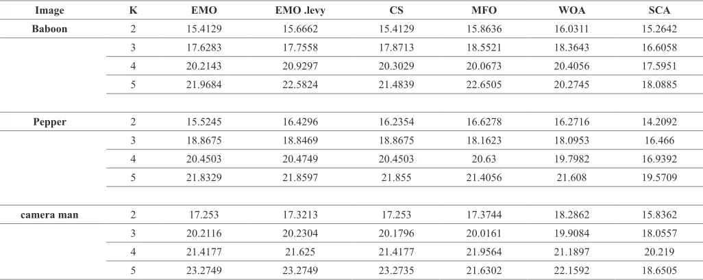
TABLE V. The Average of the Psnr Measure of All Algorithms
Image K EMO EMO .levy CS MFO WOA SCA
Baboon 2 15.4129 15.6662 15.4129 15.8636 16.0311 15.2642
3 17.6283 17.7558 17.8713 18.5521 18.3643 16.6058
4 20.2143 20.9297 20.3029 20.0673 20.4056 17.5951
5 21.9684 22.5824 21.4839 22.6505 20.2745 18.0885
Pepper 2 15.5245 16.4296 16.2354 16.6278 16.2716 14.2092
3 18.8675 18.8469 18.8675 18.1623 18.0953 16.466
4 20.4503 20.4749 20.4503 20.63 19.7982 16.9392
5 21.8329 21.8597 21.855 21.4056 21.608 19.5709
camera man 2 17.253 17.3213 17.253 17.3744 18.2862 15.8362
3 20.2116 20.2304 20.1796 20.0161 19.9084 18.0557
4 21.4177 21.625 21.4177 21.9564 21.1897 20.219
TABLE VI. CPU Time for All Algorithms (Per Second)
image k EMO.levy EMO CS WOA MFO SCA
Baboon
2 9.34 10.39 11.67 12.55 12.88 12.97
3 12.19 13.96 14.67 15.40 16.06 16.98
4 14.53 18.82 19.31 20.01 21.55 22.89
5 16.01 19.66 20.39 21.83 22.09 22.77
Pepper
2 9.67 10.31 12.31 13.95 14.33 14.87
3 12.16 14.47 15.48 15.78 16.09 16.59
4 14.78 16.26 17.45 18.66 19.23 20.01
5 16.38 18.43 19.85 20.28 21.91 22.01
Camera man
2 5.34 7.53 10.32 11.03 12.22 12.83
3 8.90 10.95 12.36 13.02 13.89 14.66
4 12.29 14.39 16.23 17.15 17.87 18.32
5 16.26 18.29 19.43 20.33 20.85 21.22
TABLE VII. Comparison Between Otsu And Kapur Thresholding Methods
Otsu method Kapur method
Image K Threshold STD PSNR Threshold STD PSNR
Baboon
2 97,149 6.92 E-13 15.6662 79, 144 1.08 E-14 15.016
3 86,126,162 7.66 E-01 17.7558 79, 143, 232 3.60 E-15 16.018
4 71,105,136,167 2.65 E-02 20.9297 44, 98, 152, 231 2.10 E-03 18.485
5 64,95,121,146,173 4.86 E-02 22.5824 33, 74, 115, 159, 231 1.08 E-14 20.507
Pepper
2 82,143 1.38 E-12 16.4296 67, 143 7.21 E-15 16.265
3 43,99,153 4.61 E-13 18.8469 62, 112, 162 2.80 E-03 18.367
4 41,89,135,175 4.61 E-13 20.4749 62, 112, 162, 227 1.28 E-01 18.754
5 39,81,119,151,183 2.33 E-02 21.8597 48, 86, 127, 171, 227 1.37 E-01 20.643
Camera man
2 70,144 1.40 E-12 17.3213 128, 196 3.60 E-15 13.626
3 57,117,155 3.07 E-01 20.2304 97, 146, 196 4.91 E-02 18.803
4 41,94,140,170 8.40 E-03 21.625 44, 96, 146, 196 1.08 E-14 20.586
5 36,83,122,149,173 2.12 E+00 23.2749 24, 60, 98, 146, 196 6.35 E-02 20.661
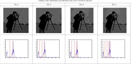
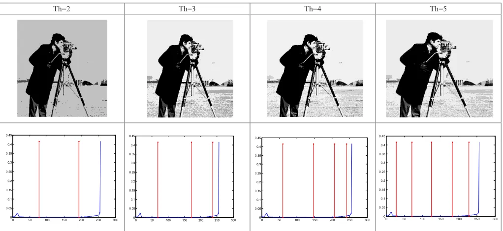
TABLE VIII. Proposed Algorithm For Low Contrast Images
Th=2 Th=3 Th=4 Th=5
0 50 100 150 200 250 300
0 0.01 0.02 0.03 0.04 0.05 0.06 0.07
0 50 100 150 200 250 300
0 0.01 0.02 0.03 0.04 0.05 0.06 0.07
0 50 100 150 200 250 300
0 0.01 0.02 0.03 0.04 0.05 0.06 0.07
0 50 100 150 200 250 300 0
Table II shows the results of segmented images after applied four optimal thresholds TH= {2,3,4,5} based on Otsu’s objective function.
Table III and Table IV show the result of the best fitness function and threshold values of three images obtained by all algorithms using Otsu’s function.
From Table III, it can be observed that the proposed algorithm (EMO.levy) has a better fitness value than other algorithms when TH={2,3,4,5} .
Table V shows that the proposed algorithm has mostly the highest values for PSNR compared to other multilevel algorithms (EMO, CS, MFO, WOA, SCA) also note whenever the number of threshold values increases, PSNR value also is increased for all algorithms.
Table VI presents the CPU time for all algorithms when applied on multilevel thresholding problem Experiments were conducted on MATLAB R2014 a running on an Intel®CoreTM i5 PC with 2.50 GHz CPU and 8 GB RAM. From this table, it can be observed that the developed algorithm gives low CPU time compared with the traditional EMO and CS algorithm.
Two multilevel thresholding-based segmentation methods; Otsu and Kapur are compared in Table VII. From this table, it can be observed that the Otsu thresholding method generates segmented images with high accuracy and higher values of PSNR and STD compared with Kapur method.
B. Low and High Contrast Test Image
In order to validate the effectiveness of the proposed algorithm, high and low contrast are applied to benchmark camera man image [36].
(a)
0 50 100 150 200 250 300 0
0.01 0.02 0.03 0.04 0.05 0.06 0.07
(b) Fig. 3. Low contrast camera man image and its histogram.
TABLE X. Result of Low Contrast Images
Comparison of Fitness values between algorithms Image K EMO.levy EMO CS
Cameraman
2 1.1517e+03 1.1516e+03 1.1516e+03
3 1.1806e+03 1.1802e+03 1.1804e+03
4 1.1922e+03 1.1923e+03 1.1922e+03
5 1.1989e+03 1.1966e+03 1.1984e+03
Comparison of thresholds values between algorithms Image k EMO.levy EMO CS
Cameraman
2 52 ,95 52,94 52,93
3 35,68,96 34,69, 96 34,67,96
4 31,66,91,104 34,68,93,106 34,68,92 106
5 29,53,77,95,107 33,67,92,104,118 32,65,87,98,109
Comparison of PSNR values between algorithms Image K EMO.levy EMO CS
Cameraman
2 21.4769 21.3387 21.4768
3 24.5621 24.4175 24.5621
4 25.6215 25.5492 25.6210
5 27.3095 25.7825 26.8439
(a) (b)
Fig. 4. High contrast camera man image and its histogram. TABLE IX. Proposed Algorithm for High Contrast Images
Th=2 Th=3 Th=4 Th=5
0 50 100 150 200 250 300 0
0.05 0.1 0.15 0.2 0.25 0.3 0.35 0.4 0.45
0 50 100 150 200 250 300 0
0.05 0.1 0.15 0.2 0.25 0.3 0.35 0.4 0.45
0 50 100 150 200 250 300 0
0.05 0.1 0.15 0.2 0.25 0.3 0.35 0.4 0.45
0 50 100 150 200 250 300 0
TABLE XI. Result Of High Contrast Images
Comparison of Fitness values between algorithms
Image K EMO.levy EMO CS
Camera man
2 9.2645e+03 9.2646e+03 8.6620e+03
3 9.3622e+03 9.3622e+03 8.7206e+03
4 9.4934e+03 9.4028e+03 8.7585e+03
5 9.4170e+03 9.4012e+03 8.7738e+03
Comparison of PSNR values between algorithms
Image k EMO.levy EMO CS
Camera man
2 18.9340 13.9395 12.8589
3 19.6216 19.5743 19.2122
4 22.3761 21.3739 20.8283
5 22.7940 22.0383 22.4284
Comparison of thresholds values between algorithms
Image K EMO.levy EMO CS
Camera man
2 77,193 78,193 73,184
3 68,171,237 68,169,236 66,163,228
4 60,147,207,241 42,108,185,238 41,106,180,232
5 28,71,125,182,228 39,100,169,218,244 37,93,154,204,236
Tables VIII, shows the proposed algorithm for low contrast images, when (th=2,3,4,5). Table IX, shows the proposed algorithm for high contrast images, (th=2,3,4,5). Table X, shows a comparative study between the proposed algorithm and other algorithms in case of low contrast images. Table XI, shows a comparative study between the proposed algorithm and other algorithms in case of high contrast images. Fig. 3 depicts the low contrast camera man image and its histogram. Fig. 4 depicts the high contrast camera man image and its histogram. From Fig. 3, 4 and Table VIII, IX, X, XI, it can be observed that the proposed algorithm still keeps with better performance compared to the other algorithms in terms of threshold, PSNR and fitness.
From the obtained results, the proposed algorithm has a powerful computational, outperforms, high converges speed, consuming less time and saves energy to perform the computational tasks. The drawback of the proposed algorithm is that the threshold and fitness function values are not usually the best for the studied cases.
V. Outstanding Features of Proposed Algorithm
In this section, the main features of the proposed optimization algorithm (EMO.levy) are summarized as follows:
• Based on the obtained results, the proposed algorithm gives the highest values for PSNR in the most studied cases compared to other algorithms (EMO, CS, MFO, WOA, and SCA) as presented in Table V.
• The proposed algorithm (EMO.levy) gives the best fitness values in the most cases compared with the other optimization algorithms when TH={2, 3, 4, 5} as presented in Table III.
• The computation time of the proposed algorithm is lower than those obtained by the other optimization techniques as presented in Table VI.
• The reliability of the proposed algorithm has been proved using different high and low contrast images.
However, the proposed optimization algorithm has a distinguished performance in the most studied cases compared with other well-known optimization algorithms. In a few cases, the PSNR and fitness values of the proposed algorithm are little bit worse than those obtained by the other optimization techniques.
VI. Conclusion
In this paper, we have proposed an improved version for electromagnetism optimization based on levy function for multilevel thresholding of image segmentation. The aim of this algorithm is to determine the best threshold values that segment the tested image accurately, producing better results compared with the original EMO version. The peak signal-to-noise ratio (PSNR) value has been used to measure the segmentation quality and similarity between original image and segmented image. The PSNR measure proved the efficiency of the algorithm compared with the other algorithms. From the experimental results of the proposed algorithm comparing with original EMO, CS, SCA, MFO and WOA algorithms, the developed algorithm has good performance regarding to the fitness function and PSNR in all images.
The future work will focus on applying the proposed optimization algorithm for higher numbers of thresholds, solving dynamic multilevel thresholding and multi-objective problems. In addition, recent optimization techniques will be applied to in order to attain better segmentation results.
References
[1] Kumar MJ, Kumar DG, Reddy RV. Review on image segmentation
techniques. International Journal of Scientific Research Engineering & Technology (IJSRET), ISSN. 2014 Sep:2278-0882.
[2] Muthukrishnan R, Radha M. Edge detection techniques for image
segmentation. International Journal of Computer Science & Information Technology. 2011 Dec 1;3(6):259.
[3] Wang Z, Ma Y, Cheng F, Yang L. Review of pulse-coupled neural
networks. Image and Vision Computing. 2010 Jan 1;28(1):5-13.
[4] Grau V, Mewes AU, Alcaniz M, Kikinis R, Warfield SK. Improved watershed
transform for medical image segmentation using prior information. IEEE transactions on medical imaging. 2004 Apr;23(4):447-58.
[5] Chuang KS, Tzeng HL, Chen S, Wu J, Chen TJ. Fuzzy c-means clustering
with spatial information for image segmentation. computerized medical imaging and graphics. 2006 Jan 1;30(1):9-15.
[6] Sezgin M, Sankur B. Survey over image thresholding techniques and
quantitative performance evaluation. Journal of Electronic imaging. 2004 Jan;13(1):146-66.
[7] Kasturi R, Goldgof D, Soundararajan P, Manohar V, Garofolo J, Bowers
R, Boonstra M, Korzhova V, Zhang J. Framework for performance evaluation of face, text, and vehicle detection and tracking in video: Data, metrics, and protocol. IEEE Transactions on Pattern Analysis and Machine Intelligence. 2009 Feb;31(2):319-36.
[8] Sauvola J, Pietikäinen M. Adaptive document image binarization. Pattern
recognition. 2000 Feb 29;33(2):225-36.
[9] Du S, Ibrahim M, Shehata M, Badawy W. Automatic license plate
recognition (ALPR): A state-of-the-art review. IEEE Transactions on circuits and systems for video technology. 2013 Feb;23(2):311-25.
[10] Bazi Y, Bruzzone L, Melgani F. Image thresholding based on the EM
algorithm and the generalized Gaussian distribution. Pattern Recognition. 2007 Feb 1;40(2):619-34.
[11] Hammouche K, Diaf M, Siarry P. A comparative study of various
meta-heuristic techniques applied to the multilevel thresholding problem. Engineering Applications of Artificial Intelligence. 2010 Aug 1;23(5):676-88.
[12] Cheng HD, Chen YH, Jiang XH. Thresholding using two-dimensional
histogram and fuzzy entropy principle. IEEE Transactions on Image Processing. 2000 Apr;9(4):732-5.
[13] Zahara E, Fan SK, Tsai DM. Optimal multi-thresholding using a
hybrid optimization approach. Pattern Recognition Letters. 2005 Jun 30;26(8):1082-95.
[14] Zhang J, Hu J. Image segmentation based on 2D Otsu method with
histogram analysis. In Computer Science and Software Engineering, 2008 International Conference on 2008 Dec 12 (Vol. 6, pp. 105-108). IEEE.
[15] Manic KS, Priya RK, Rajinikanth V. Image multithresholding based on
[16] Bhandari AK, Kumar A, Singh GK. Modified artificial bee colony based computationally efficient multilevel thresholding for satellite image segmentation using Kapur’s, Otsu and Tsallis functions. Expert Systems with Applications. 2015 Feb 15;42(3):1573-601.
[17] Kennedy J. Particle swarm optimization. InEncyclopedia of machine
learning 2011 (pp. 760-766). Springer US.
[18] El Aziz MA, Ewees AA, Hassanien AE. Whale Optimization Algorithm
and Moth-Flame Optimization for multilevel thresholding image segmentation. Expert Systems with Applications. 2017 Oct 15; 83:242-56.
[19] Elsayed SM, Sarker RA, Essam DL. A new genetic algorithm for solving
optimization problems. Engineering Applications of Artificial Intelligence. 2014 Jan 1; 27:57-69.
[20] Tao W, Jin H, Liu L. Object segmentation using ant colony optimization
algorithm and fuzzy entropy. Pattern Recognition Letters. 2007 May 1;28(7):788-96.
[21] Birbil Şİ, Fang SC. An electromagnetism-like mechanism for global
optimization. Journal of global optimization. 2003 Mar 1;25(3):263-82.
[22] Guan X, Dai X, Li J. Revised electromagnetism-like mechanism for
flow path design of unidirectional AGV systems. International Journal of Production Research. 2011 Jan 15;49(2):401-29.
[23] Jhang JY, Lee KC. Array pattern optimization using electromagnetism-like
algorithm. AEU-International Journal of Electronics and Communications. 2009 Jun 1;63(6):491-6.
[24] Lee CH, Chang FK. Fractional-order PID controller optimization
via improved electromagnetism-like algorithm. Expert Systems with Applications. 2010 Dec 1;37(12):8871-8.
[25] Yurtkuran A, Emel E. A new hybrid electromagnetism-like algorithm for
capacitated vehicle routing problems. Expert Systems with Applications. 2010 Apr 1;37(4):3427-33.
[26] Hung HL, Huang YF. Peak to average power ratio reduction of multicarrier
transmission systems using electromagnetism-like method. Int J Innov Comput Inf Control. 2011 May 1;7(5A):2037-50.
[27] Naderi B, Tavakkoli-Moghaddam R, Khalili M. Electromagnetism-like
mechanism and simulated annealing algorithms for flowshop scheduling problems minimizing the total weighted tardiness and makespan. Knowledge-Based Systems. 2010 Mar 1;23(2):77-85.
[28] Cuevas E, Oliva D, Zaldivar D, Pérez-Cisneros M, Sossa H. Circle
detection using electro-magnetism optimization. Information Sciences. 2012 Jan 1;182(1):40-55.
[29] Birbil Şİ, Fang SC, Sheu RL. On the convergence of a population-based
global optimization algorithm. Journal of global optimization. 2004 Nov 1;30(2-3):301-18.
[30] Oliva D, Cuevas E, Pajares G, Zaldivar D, Osuna V. A multilevel thresholding algorithm using electromagnetism optimization. Neurocomputing. 2014 Sep 2; 139:357-81.
[31] Suresh S, Lal S. An efficient cuckoo search algorithm based multilevel
thresholding for segmentation of satellite images using different objective functions. Expert Systems with Applications. 2016 Oct 1; 58:184-209. [32] Suresh, S., Lal, S., Chen, C., & Celik, T. Multispectral Satellite Image
Denoising via Adaptive Cuckoo Search-Based Wiener Filter. IEEE Transactions on Geoscience and Remote Sensing. 2018 99:1-12.
[33] Mirjalili S. SCA: a sine cosine algorithm for solving optimization
problems. Knowledge-Based Systems. 2016 Mar 15;96:120-33. [34] Yildiz S., Yildiz, R. comparison of grey wolf, whale, water cycle, ant
lion and sine-cosine algorithms for the optimization of a vehicle engine connecting rod. Materials Testing, 2018, 60.3: 311-315.
[35] Pavlyukevich I. Lévy flights, non-local search and simulated annealing.
Journal of Computational Physics. 2007 Oct 1;226(2):1830-44.
[36] Martin D, Fowlkes C, Tal D, Malik J. A database of human segmented
natural images and its application to evaluating segmentation algorithms and measuring ecological statistics. InComputer Vision, 2001. ICCV 2001. Proceedings. Eighth IEEE International Conference on 2001 (Vol. 2, pp. 416-423). IEEE. 2004 Jan;13(1):146-66.
Ashraf M. Hemeida
Ashraf Mohamed Hemeida, was born in Elmenia, Egypt. He obtained his B.Sc., and M.Sc. in electrical engineering from Faculty of Engineering, Elminia University, Elmenia, Egypt in 1992 and 1996 respectively. In Nov. 1992, he engaged Higher Institute of Energy, Aswan as Teaching Assistant. From 1998 to 1999 he was a full time Ph.D. student with Electrical and Computer Engineering Department, University of New Brunswick, Canada. In Sept., 2000 he obtained his Ph.D. From Electrical Engineering Department, Faculty of Engineering, Assiut University, Assiut Egypt. From Oct. 2000 till August 2005 he was assistant professor at Electrical Engineering Department, Higher Institute of Energy, South Valley University, Aswan, Egypt. In Nov. 2005 he obtained associate professor rank. Dr. Hemeida is a full professor since July, 2011. His research interest artificial intelligence applications, optimization techniques, fuzzy systems, image processing, and advanced control techniques in electrical systems. Professor Hemeida is a member of editorial board of ARPN Journal of Engineering and Applied Sciences.
Radwa Mansour
Radwa, Mansour received the B.Sc. degree in computer science from the Faculty of Science, Aswan University, Aswan, Egypt, in 2011. Her research interests include artificial intelligence applications, optimization techniques, fuzzy systems, and image processing.
Mohamed Eid Hussein