The Relationship Between Agnostic Selective Classification,
Active Learning and the Disagreement Coefficient
Roei Gelbhart [email protected]
Department of Computer Science
Technion — Israel Institute of Technology
Ran El-Yaniv [email protected]
Department of Computer Science
Technion — Israel Institute of Technology
Editor:Gabor Lugosi
Abstract
A selective classifier (f, g) comprises a classification functionf and a binary selection func-tiong, which determines if the classifier abstains from prediction, or usesf to predict. The classifier is called pointwise-competitive if it classifies each point identically to the best classifier in hindsight (from the same class), whenever it does not abstain. The quality of such a classifier is quantified by its rejection mass, defined to be the probability mass of the points it rejects. A “fast” rejection rate is achieved if the rejection mass is bounded from above by ˜O(1/m) wheremis the number of labeled examples used to train the clas-sifier (and ˜O hides logarithmic factors). Pointwise-competitive selective (PCS) classifiers are intimately related to disagreement-based active learning and it is known that in the realizable case, a fast rejection rate of a known PCS algorithm (called Consistent Selective Strategy) is equivalent to an exponential speedup of the well-known CAL active algorithm. We focus on the agnostic setting, for which there is a known algorithm called LESS that learns a PCS classifier and achieves a fast rejection rate (depending on Hanneke’s disagreement coefficient) under strong assumptions. We present an improved PCS learning algorithm called ILESS for which we show a fast rate (depending on Hanneke’s disagree-ment coefficient) without any assumptions. Our rejection bound smoothly interpolates the realizable and agnostic settings. The main result of this paper is an equivalence between the following three entities: (i) the existence of a fast rejection rate for any PCS learning algorithm (such as ILESS); (ii) a poly-logarithmic bound for Hanneke’s disagreement coef-ficient; and (iii) an exponential speedup for a new disagreement-based active learner called Active-ILESS.
Keywords: active learning, selective prediction, disagreement coefficient, selective sam-pling, selective classification, reject option, pointwise-competitive, selective classification, statistical learning theory, PAC learning, sample complexity, agnostic case
1. Introduction
Selective classification is a unique and extreme instance of the broader concept of confidence-rated prediction (Chow, 1970; Vovk et al., 2005; Bartlett and Wegkamp, 2008; Yuan and Wegkamp, 2010; Cortes et al., 2016a; Wiener and El-Yaniv, 2012; Kocak et al., 2016; Zhang and Chaudhuri, 2014). Given a training sample consisting of m labeled
in-c
stances, the learning algorithm is required to output a selective classifier (El-Yaniv and Wiener, 2010), defined to be a pair (f, g), where f is a prediction function, chosen from some hypothesis class F, and g :X → {0,1} is a selection function, serving as a qualifier for f as follows: for any x, if g(x) = 1, the classifier predicts f(x), and otherwise it ab-stains. The general performance of a selective classifier is quantified in terms of itscoverage
and risk, where coverage is the probabilistic mass of non-rejected instances, and risk is the normalized average loss off restricted to non-rejected instances. Letf∗ be any (unknown) true risk minimizer1 inF for the given problem. The selective classifier (f, g) is said to be
pointwise-competitive if, for each x with g(x) = 1, it must hold that f(x) = f∗(x) for all
f∗ ∈ F (Wiener and El-Yaniv, 2015). Thus, pointwise-competitiveness w.h.p. over choices of the training sample, is a highly desirable property: it guarantees, for each non-rejected test point, the best possible classification obtainable using the best in-hindsight classifier fromF. We do not restrictgto be from any specific hypothesis class, however, because we use disagreement-based selective prediction, the selection ofF will limit the possibilities of
g. The scenario of a predefined decision functions hypothesis class is investigated in Cortes et al. (2016b).
Pointwise-competitive selective classification (PCS) was first considered in the realizable case (El-Yaniv and Wiener, 2010), for which a simple consistent selective strategy (CSS) was shown to achieve a bounded and monotonically increasing (withm) coverage in various non-trivial settings. Note that in the realizable case, any PCS strategy attains zero risk (over the sub-domain it covers). These results were recently extended to the agnostic setting (Wiener and El-Yaniv, 2015; El-Yaniv and Wiener, 2011) with a related but different algorithm called low-error selective strategy (LESS), for which a number of coverage bounds were shown. These bounds relied on the fact that the underlying probability distribution and the hypothesis classF will satisfy the so-called “(β1, β2)-Bernstein property” (Bartlett et al., 2004). The coverage bounds used by Wiener and El-Yaniv (2015); El-Yaniv and Wiener (2011) are dependent on the parameters β1, β2. This Bernstein property assumption (as presented in Bartlett et al., 2004), which allows for better concentration, nevertheless, can be problematic. First, it is defined with respect to a unique true risk minimizer f∗, a property that is unlikely to hold in noisy agnostic settings. Moreover, for arbitraryF, even for the 0/1 loss function,there is little knowledge about cases for which the property holds with a non-trivialβ2.2 We removed the Bernstein assumption from our analysis.
Assuming that a selective classifier is w.h.p. pointwise-competitive, our key goal is a small rejection rate. We will say that a learner has afast R∗ rejection rate, if w.h.p. the rejection rate is bounded by
polylog
1
R(f∗) + 1/m
·R(f∗) +d·polylog(m,1/δ)
m ,
1. We assume that there exists an f∗ inF. Otherwise, we can artificially define f∗ to be any function whose risk is sufficiently close to inff∈F(R(f)), for instance, not greater than a small additive factor
from this infimum.
whereR(f∗),dandδ are defined in Section 2. Selective classification is very closely related to the field of active learning (AL). In active learning, the learner can actively influence the learning process by selecting the points to be labeled. The incentive for introducing this extra flexibility is to reduce labeling efforts. A key question in theoretical studies of AL is how many label requests are sufficient to learn a given (unknown) target concept to a specified accuracy, a quantity called label complexity. For an AL algorithm satisfying the “passive example complexity” property (consuming the same number of unlabeled (and labeled) examples, as a passive algorithm consumes labeled examples for achieving the same error; see Definition 6.2), we will say it hasR∗ exponential speedup, if w.h.p. the number of labels it requests is bounded by
polylog
1
R(f∗) + 1/m
·R(f∗)m+d·polylog(m,1/δ).
The connection between active learning and confidence-rated prediction is quite intu-itive. A pointwise-competitive selective classifier P can be straightforwardly used as the querying component of an active learning algorithm. This reduction is most naturally demonstrated in the stream-based AL model: at each iteration, the active algorithm trains a selective classifier on the currently available labeled samples, and then decides to query a newly introduced (unlabeled) pointx ifP abstains on x.
Hanneke’s disagreement coefficient (Hanneke, 2007), see Definition 2.1, is a well-known parameter of the hypothesis class and the marginal distribution; it is used in most of the known label complexity bounds (Hsu, 2010; Hanneke, 2007; Ailon et al., 2012). The disagreement coefficient is the supremum of the relation between the disagreement mass of functions that are r-distanced from f∗ to r, over r. PCS classification is based on using generalization bounds to estimate the empirical error of f∗, and more specifically, its distance from the empirical error of the ERM. Whenever all the functions that reside within a ball around the ERM unanimously agree, the classifier chooses to classify. Thus, the abstain rate is dependent on the disagreement mass of the functions within the ball. The radius of the ball depends on the generalization bounds. The generalization bounds we use are of the form ˜O(R(f∗) +d/m) for the agnostic case. After observing mexamples, we can bound the disagreement mass of a ball around the ERM, by multiplying the radius of the ball, which is ˜O(R(f∗) +d/m), with the disagreement coefficient. Thus, if for example, the disagreement coefficient is bounded by a constant, the abstain rate of some PCS algorithms can be bounded by ˜O(R(f∗) +d/m). This gives a basic idea of the disagreement coefficient, which will be formally presented later on.
Note that, in principle, the disagreement coefficient can be replaced by another im-portant quantity, namely, the version space compression set size, recently shown to be equivalent to it (Wiener et al., 2015; El-Yaniv and Wiener, 2015). Specifically, an
O(polylog(m)log(1/δ)) version space compression set size minimal bound was shown by Wiener et al. (2015, Corollary 11), to be equivalent to an O(polylog(1/r)) disagreement coefficient.
show that for the case of linear classification under log-concave distributions, their analysis can improve (reduce) the argument inside the logarithm of the label complexity bound, and the dependency on the VC-dimension is also reduced by a square root. However, in our paper we focus mainly on the more basic question: when can we achieve an exponential speedup in terms of 1/. Thus, due to the simplicity of the disagreement coefficient, and its widespread use in the literature, we chose to focus on it. See a detailed discussion on the
ϕcquantity in Section 9.
The first contribution of this paper is a novel selective classifier, called ILESS, which uses a tighter generalization error bound than LESS and depends on R(f∗) (and interpolates the agnostic and realizable cases). Most importantly, the new strategy can be analyzed completely without the Bernstein condition.
We derive an active learning algorithm, called Active-ILESS, corresponding to our selec-tive classifier, ILESS. Acselec-tive-ILESS is constructed to work in a stream-based AL model and its querying function is extremely conservative: for each unlabeled example, the algorithm requests its label if and only if the labeling of the optimal classifier (from the same class) on this point cannot be inferred from information already acquired. This querying strategy, which is often termed “disagreement-based,” has been used in a number of stream-based AL algorithms such as Agnostic CAL and Oracular CAL (Hsu, 2010),A2(Agnostic Active), developed by Balcan et al. (2006), RobustCAL, studied in Hanneke (2012, 2014b) and Han-neke and Yang (2012), or the general agnostic AL algorithm of Dasgupta et al. (2007). Paper Huang et al. (2015) presented a computationally efficient algorithm for disagreement-based AL.
We prove that Active-ILESS, despite being very similar to Oracular CAL Hsu (2010), exhibits an improved label complexity, in comparison to that proved for Oracular CAL. Specifically, Active-ILESS achieves the same label complexity as Agnostic CAL, while being simpler in the sense that its consumption of ERM computations is smaller.
The first formal relationship between PCS classification and AL was proposed by El-Yaniv and Wiener (2012); Wiener (2013), where the aforementioned CSS algorithm was shown to be equivalent to the well-known CAL AL algorithm of Cohn et al. (1994), in the sense that a fast coverage rate for CSS was proven to be equivalent to an exponential label complexity speedup for CAL. This result applies to the realizable setting only. Our first contribution is a similar equivalence relation between pointwise-competitive selective classification and AL, which applies to the more challenging agnostic case and smoothly interpolates the realizable and agnostic settings.
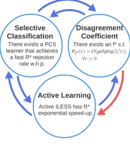
Our second and main contribution is to show a complete equivalence between (i) selective classification with a fast R∗ rejection rate, (ii) an AL algorithm, Active-ILESS, with an
R∗ exponential speedup, and (iii) the existence of an f∗ with a disagreement coefficient bounded by polylog(1/r). This is illustrated in Figure 1, where the blue errors indicate the equivalence relationships we prove in this paper, and the red arrow indicates a previously known result (Hsu, 2010; Hanneke, 2007), and can also be deduced from the other arrows.
2. Definitions
Figure 1: Main results
of labeled training examples Sm = ((x1, y1),(x2, y2), ...,(xm, ym)), such that ∀i,(xi, yi) ∈ X × Y, the empirical error of a hypothesis f over Sm is ˆR(f, Sm) , m1 Pmi=1`(f(xi), yi),
where`:Y × Y →R+is a loss function. In this paper, we focus mainly on the zero-one loss
function, `01(y, y0),1{y6=y0}. The true (zero-one) error off is R(f),EP[`01(f(x), y)]. An empirical risk minimizer hypothesis (henceforth, an ERM) is
ˆ
f(Sm),argmin f∈F
ˆ
R(f, Sm), (1)
and a true risk minimizer isf∗ ,argminf∈FR(f).3
We acquire the following definitions from Wiener and El-Yaniv (2015). For any hypoth-esis classF, hypothesisf ∈ F, distributionPX,Y, sampleSm, and real numberr >0, define
the true and empirical low-error sets,
V(f, r),f0 ∈ F :R(f0)≤R(f) +r (2)
and
ˆ
V(f, r),nf0 ∈ F : ˆR(f0, Sm)≤Rˆ(f, Sm) +r
o
. (3)
Let G ⊆ F. The disagreement set (Hanneke, 2007) and agreement set (El-Yaniv and Wiener, 2010) w.r.t. G are defined, respectively, as
DIS(G),{x∈ X :∃f1, f2∈G , f1(x)6=f2(x)} (4)
and AGR(G),{x∈ X :∀f1, f2∈G , f1(x) =f2(x)}. (5) In selective classification (El-Yaniv and Wiener, 2010), the learning algorithm receives Sm
and is required to output aselective classifier, defined to be a pair (f, g), where f ∈ F is a classifier, and g:X → {0,1} is aselection function, serving as a qualifier for f as follows. For any x ∈ X, (f, g)(x) = f(x) iff g(x) = 1. Otherwise, the classifier outputs “I don’t know”. For any selective classifier (f, g), we define its coverage to be
Φ(f, g), Pr
X∼PX
(g(X) = 1),
and its complement, 1−Φ, is called the abstain rate. For any f ∈ F and r > 0, define the set B(f, r) of all hypotheses that reside within a ball of radius r around f,
B(f, r),
f0 ∈ F : Pr
X∼PX
f0(X)6=f(X) ≤r
.
For anyG⊆ F, and distributionPX, we denote by ∆Gthe volume of the disagreement set of G(see (4)), ∆G,Pr{DIS(G)}.
Definition 2.1 (Disagreement Coefficient) Let r0 ≥0. Hanneke’s disagreement coef-ficient (Hanneke, 2007) of a classifier f ∈ F with respect to the target distribution PX is
θf(r0), sup r>r0
∆B(f, r)
r , (6)
and the general disagreement coefficientof the entire hypothesis class F is
θ(r0),sup
f∈F
θf(r0). (7)
Notice that this definition of the disagreement coefficient is independent of PY|X. An-other commonly used definition of the disagreement coefficient does depend on a true risk minimizerf∗, as follows:
θ0(r0) = sup
r>r0
∆B(f∗, r)
r . (8)
3. Convergence Bounds and LESS
We use a uniform convergence bound from Vapnik and Chervonenkis (1974); Dasgupta et al. (2007); Bousquet et al. (2003). Define convergence slacks σR−Rˆ(m, δ, d, R,Rˆ) and
σRˆ−R(m, δ, d, R,Rˆ), given in terms of the training sample, Sm, its size, m, the confidence parameter, δ, and the VC-dimensiondof the classF. For anyf ∈ F,
σR−Rˆ(m, δ, d, R,Rˆ),min
4dln(16dδme)
m +
s
4dln(16dδme)
m ·
ˆ
R
| {z }
ˆ
σR−Rˆ(m,δ,d,Rˆ)
,
s
4dln(16dδme)
m ·R
| {z }
¯
σR−Rˆ(m,δ,d,R)
(9) and
σRˆ−R(m, δ, d, R,Rˆ),min
4dln(16dδme)
m +
s
4dln(16dδme)
m ·R
| {z }
¯
σRˆ−R(m,δ,d,R)
,
s
4dln(16dδme)
m ·Rˆ
| {z }
ˆ
σRˆ−R(m,δ,d,Rˆ)
. (10)
To simplify the analysis, we further decompose the above slack terms into their empirical and non-empirical components. For (9), we thus have, respectively,
ˆ
σR−Rˆ(m, δ, d,Rˆ),
4dln(16dδme)
m +
s
4dln(16dδme)
m ·
ˆ
R (11)
and
ˆ
σRˆ−R(m, δ, d,Rˆ),
s
4dln(16dδme)
m ·R.ˆ (12)
Similarly, the non-empirical part in these minimums are denoted by ¯σR−Rˆ and ¯σRˆ−R. With this notation, we can write, for example,σR−Rˆ = min{σˆR−Rˆ,σ¯R−Rˆ}. Our Lemma 1 is taken from the work of Dasgupta et al. (2007, Lemma 1), which is based on Bousquet et al. (2003, Theorem 7)4.
Lemma 1 Let F be a hypothesis class with VC-dimension d. For any 0 < δ < 1, with probability of at least1−δ over the choice ofSm fromPm, any hypothesis f ∈ F satisfies
R(f)≤Rˆ(f) +σR−Rˆ
m, δ, d, R(f),Rˆ(f) (13)
ˆ
R(f)≤R(f) +σRˆ−R
m, δ, d, R(f),Rˆ(f). (14)
4. In the original lemma from Dasgupta et al. (2007),S(H, n), the growth function, is given. We insert Sauer’s Lemma,S(H, n)≤(em
d ) d
Strategy 1 is the LESS algorithm of Wiener and El-Yaniv (2015). LESS learns w.h.p. a pointwise-competitive selective classifier, (f, g), where f ∈ F and g : X → {0,1} is its selection function that determines whether to abstain or to classify. Apointwise-competitive selective classifier must satisfy the following condition: For each x with g(x) = 1, it must hold that f(x) = f∗(x) for all f∗ ∈ F. A PCS learning algorithm must output a PCS classifier w.h.p. for all PY|X; otherwise, one can consider a tailor-made trivial algorithm for each distribution, which simply returnsf∗.
Remark 2 The original definition of pointwise-competitiveness from Wiener and El-Yaniv (2015) requires a single f∗. We widen the definition to cases for which there are more than one f∗, and require that a pointwise-competitive selective classifier be equal to all f∗, wherever g= 1. This extrapolation seems a bit strict. Nevertheless, even if the requirement would have been relaxed to “any f∗”, any pointwise-competitive selective classifier would still have been forced to identify with all f∗, as it is impossible to determine whether a set of functions are all f∗, or one is better than the rest.
The main idea behind LESS is that, w.h.p., all f∗ lie within a ball around an ERM hypothesis with an error radius of 2σ(m, δ/4, d), where
σ(m, δ, d),2
s
2d ln2med + ln2δ
m (15)
is the slack term of a certain uniform convergence bound. Therefore, if all the functions in that ball agree over the labeling of any instancex, we know with high probability that allf∗
labelxthe same way as the ERM. This property ensures that LESS is pointwise-competitive w.h.p.
Strategy 1Agnostic Low-Error Selective Strategy (LESS) Input: Sample set of sizem,Sm,
Confidence levelδ
Hypothesis classF with VC dimensiond Output: A selective classifier (h, g)
1: Set ˆf=ERM(F, Sm), i.e., ˆf is any empirical risk minimizer fromF
2: SetG= ˆVf ,ˆ2σ(m, δ/4, d)
3: Constructgsuch thatg(x) = 1⇐⇒x∈ {X \DIS(G)} 4: f = ˆf
4. ILESS
We now introduce an improved version of LESS, called ILESS, which uses a radius of
the form d·polylog(m,1/δ)·
1
m +
q
R(f∗)
m
. Noting that the radius, 2σ(m, δ/4, d), used
by LESS to define G= ˆV, is of the formd·polylog(m,1/δ)/√m, we observe that in cases whereR(f∗)≈ C
m, this new radius behaves as
d·polylog(m,1/δ)
m . We later show that this radius
Strategy 2Improved Low-Error Selective Strategy (ILESS) Input: Sample set of sizem,Sm,
Confidence levelδ
Hypothesis classF with VC dimensiond Output: A selective classifier (h, g)
1: Set ˆf=ERM(F, Sm), i.e., ˆf is any empirical risk minimizer fromF
2: SetσILESS= ˆσR−Rˆ
m, δ, d,Rˆ( ˆf , Sm)
+ ¯σRˆ−R
m, δ, d,Rˆ( ˆf , Sm) + ˆσR−Rˆ(m, δ, d,Rˆ( ˆf , Sm))
3: SetG= ˆVf , σˆ ILESS
4: Constructgsuch thatg(x) = 1⇐⇒x∈ {X \DIS(G)} 5: h= ˆf
for which g(x) = 1, f(x) = f∗(x) for all f∗. The calculation of g appears to be very problematic, as for a specific x, a unanimous decision over an infinite number of functions must be ensured. This problem was shown to be reducible to finding an ERM under one constraint (Lemma 6.1 in El-Yaniv and Wiener, 2011, a.k.a. the disbelief principle). This is a difficult problem, nonetheless, albeit one that could be estimated with heuristics.
Definition 4.1 Let F be a hypothesis class with a finite VC dimension d, and PX,Y be an
unknown probability distribution. Given a sample setSm, drawn fromPX,Y, we denote by E
the event where both inequalities (13) and (14) of Lemma 1 simultaneously hold. We know from the lemma that E occurs with probability of at least1−δ.
Lemma 3 (ILESS is pointwise-competitive) Given that event E occurred (see Defini-tion 4.1), for all f∗ ∈ F, f∗ resides within G (from Strategy 2), and therefore, ILESS is pointwise-competitive w.h.p.
Proof From (14), it follows that ˆ
R(f∗, Sm) ≤ R(f∗) +σRˆ−R(m, δ, d, R(f
∗),Rˆ(f∗, S
m))
≤ R(f∗) + ¯σRˆ−R(m, δ, d, R(f
∗)). (16)
Additionally, by the definition of f∗, we know that it has the lowest true error, and using Inequality (13) from Lemma 1 we obtain,
R(f∗) ≤ R( ˆf)
≤ Rˆ( ˆf , Sm) +σR−Rˆ(m, δ, d, R( ˆf),Rˆ( ˆf , Sm))
≤ Rˆ( ˆf , Sm) + ˆσR−Rˆ(m, δ, d,Rˆ( ˆf , Sm)). (17) Finally, by applying (17) in (16), we have,
ˆ
R(f∗, Sm)≤Rˆ( ˆf , Sm) + ˆσR−Rˆ(m, δ, d,Rˆ( ˆf , Sm))
+ ¯σRˆ−R
m, δ, d,Rˆ( ˆf , Sm) + ˆσR−Rˆ(m, δ, d,Rˆ( ˆf , Sm))
,
Lemma 4 below bounds the radius σILESS of ILESS. The lemma uses the notation
A,4dln(16me
dδ ),
with which, by the definition of σILESS (see Strategy 2), we have,
σILESS = σˆR−Rˆ(m, δ, d,Rˆ( ˆf , Sm)) + ¯σRˆ−R
m, δ, d,Rˆ( ˆf , Sm) + ˆσR−Rˆ(m, δ, d,Rˆ( ˆf , Sm))
= A
m+
r
A
m ·Rˆ( ˆf , Sm) + A m +
v u u t
A m ·
"
ˆ
R( ˆf , Sm) + A m +
r
A
m ·Rˆ( ˆf , Sm)
#
.
(18)
Lemma 4 Given that event E (see Definition 4.1) occurred, the radius ofILESS satisfies
σILESS ≤6
A m + 3
r
A m ·R(f
∗) =O A
m +
r
A m ·R(f
∗)
!
, (19)
where A,4dln(16dδme).
Proof Under our assumption, inequalities (13) and (14) hold for every f ∈ F. We thus have
ˆ
R( ˆf , Sm)≤Rˆ(f∗, Sm)≤R(f∗) + A
m +
r
A m·R(f
Replacing the three occurrences of ˆR(f∗, Sm) in (18) with the R.H.S. of (20), and using the
basic inequalities√a+b≤√a+√b and√ab≤a/2 +b/2, we get,
σILESS ≤
A m + v u u t A
m · R(f
∗) + A
m +
r
A m ·R(f
∗) ! + A m + + v u u u t A m ·
R(f∗) +
2A
m +
r
A m ·R(f
∗) + v u u t A
m· R(f
∗) + A
m +
r
A m·R(f
∗)
!
≤ 2A
m +
s
A m ·
R(f∗) + A
m + A
2m+
1 2R(f
∗) + + v u u tA m · "
R(f∗) + 3A 2m +
1 2R(f
∗) + A
m+
s
A m ·
R(f∗) + 3A 2m +
1 2R(f
∗)
#
≤ 2A
m +
3A
2m +
3 2
r
A mR(f
∗) + v u u tA m · " 5A
2m +
3 2R(f
∗) + s A m · 3A
2m +
3 2R(f
∗)
#
≤ 7A 2m +
3 2
r
A m ·R(f
∗) + v u u t A m· " 5A
2m +
3 2R(f
∗) + 3A 2m +
r
3A
2m·R(f
∗)
#
≤ 7A 2m +
3 2
r
A m ·R(f
∗) + s A m· 5A
2m +
3 2R(f
∗) + 3A 2m +
3A
4m +
3 4R(f
∗)
≤ 7A 2m +
3 2
r
A m ·R(f
∗) + r 19 4 A m+ r A m · 9 4R(f
∗)
≤ 6A
m + 3
r
A m ·R(f
∗). (21)
In comparison, the radius of LESS is of order O(
q
A
m), which can be significantly larger
when R(f∗) is small. This potential radius advantage translates into a potential coverage advantage of ILESS, as stated in the following theorem.
Theorem 5 Let F be a hypothesis class with a finite VC dimension d, and let PX,Y be
an unknown probability distribution. Given that event E (see Definition 4.1) occurred, G defined in Strategy 2, holds that
G⊆B(f∗, R0),
where
R0 ,2·R(f∗) + 11·
A m + 6·
r
A m·R(f
∗),
and thus, for allf∗, the abstain rate is bounded by
This immediately implies (by definition) that
1−Φ(ILESS)≤θ(R0)·R0. Remark 6 Note that R0 =O R(f∗) +mA
due to
q
A
m ·R(f∗)≤
1 2(
A m +R(f
∗)).
Proof We start by showing thatG, defined in Strategy 2, resides within a ball around any specific f∗. To do so, we need to bound the true error of all functions in G.
f ∈G ⇒ Rˆ(f, Sm)≤Rˆ( ˆf , Sm) +σILESS (22) ⇒ Rˆ(f, Sm)≤R(f∗) +
A m+
r
A m ·R(f
∗) + 6A
m + 3
r
A m ·R(f
∗) (23)
⇒ Rˆ(f, Sm)≤R(f∗) + 7· A m+ 4·
r
A m ·R(f
∗), (24)
where Inequality (22) is explained by the definition of G, and inequality (23) follows from (20) and (21) (under event E). We then have,
R(f) ≤ Rˆ(f, Sm) + ˆσR−Rˆ(m, δ, d,Rˆ) (25) ≤ Rˆ(f, Sm) +
A m +
r
A
m ·Rˆ(f, Sm) (26)
≤ R(f∗) + 8· A
m + 4·
r
A m ·R(f
∗) + + v u u t A m· "
R(f∗) + 7· A
m + 4·
r
A m ·R(f
∗)
#
(27)
≤ R(f∗) + 8· A
m + 4·
r
A m ·R(f
∗) +
s
A m ·
3R(f∗) + 9· A
m
(28)
≤ R(f∗) + 11· A
m + 6·
r
A m ·R(f
∗), (29)
where inequality (25) is (13) (which holds given E), inequality (26) follows directly from the definition of ˆσR−Rˆ, inequality (27) is obtained using (24), Inequality (28) follows from √
ab≤a/2 +b/2, and (29) from √a+b≤√a+√b. Using (29), for all f ∈G, and any f∗, we have,
Pr
X∼PX
{f(X)6=f∗(X)} = Pr
X,Y∼PX,Y
{f(X)6=f∗(X)∧f∗(X) =Y}+
Pr
X,Y∼PX,Y
{f(X)6=f∗(X)∧f∗(X)6=Y}
≤ Pr
X,Y∼PX,Y
{f(X)6=f∗(X)∧f∗(X) =Y}+R(f∗)
≤ Pr
X,Y∼PX,Y
{f(X)6=Y}+R(f∗)
= R(f) +R(f∗)
≤ 2·R(f∗) + 11· A
m + 6·
r
A m·R(f
It follows that
f ∈B f∗,2·R(f∗) + 11· A
m + 6·
r
A m ·R(f
∗)
!
=B(f∗, R0),
and, in particular,
G⊆B(f∗, R0), so,
∆G≤∆B(f∗, R0).
The abstain rate of ILESS equals ∆G. We can now use the disagreement coefficient to bound the abstain rate from above,
∆G≤∆B(f∗, R0) = ∆B(f ∗, R0)
R0
·R0≤θ(R0)·R0, (31) which concludes the proof.
According to Theorem 5, assuming the disagreement coefficient isθ(r) =O(polylog(1/r)) for r ≥ R(f∗), the rejection mass of ILESS, defined as the probability that the classifier trained by ILESS will output “I don’t know” is bounded w.h.p. by
polylog1
1
R(f∗) + 1/m
·R(f∗) +d·polylog2(m,1/δ)
m . (32)
In many cases, the disagreement coefficient, θ(r), is bounded by a constant, or by
O(polylog(1/r)) for all r >0 (see Hanneke, 2014b). For example, it was shown in Wiener et al. (2015), that for linear separators under mixture of Gaussians, and for axis-aligned rectangles with probability mass bounded away from zero under product densities overRk, θ(r) is bounded by O(polylog(1/r)) for allr >0. For such cases, we know that (32) always holds, regardless of the size of R(f∗). The disagreement coefficient is only dependent on the marginal PX, the hypothesis class F, and the identity of the true risk minimizers, f∗ (which is not necessarily unique). This fact motivates the following definition of a rejection rate of a selective learning algorithm, which is only dependent on PX,F and f∗.
Definition 4.2 (Fast R∗ Rejection Rate) Given PX,F and f∗, if for all δ > 0, and
all PY|X for which f∗ is a true risk minimizer, the rejection mass of a selective classifier learning algorithm is bounded by (32) with probability of at least 1−δ, we say that the algorithm achieves afast R∗ rejection rate, withpolylog1 andpolylog2 as its parameters.
Corollary 7 Let F be a hypothesis class with a finite VC dimension d. Given PX and
f∗, if θf∗(r) is bounded by O(polylog(1/r)) for all r >0, then there exists a PCS learning
algorithm (ILESS) which achieves a fastR∗ rejection rate.
Proof The proof is immediate from Theorem 5.
As long as the number of training examples that ILESS receives is not “too large” relative to 1/R(f∗), i.e., m R(1f∗), the rejection mass of ILESS is
O
d·polylog(m,1/δ)
m
.
Whenmis large, andR(f∗) becomes more dominant thanm1, our coverage bound is dom-inated by R(f∗). This should not surprise us, as ILESS achievespointwise-competitiveness
w.h.p., and any strategy that achieves pointwise-competitiveness cannot ensure a better rejection mass thanR(f∗) without making more assumptions about the error or the distri-bution. This can be seen in the following example, in which θ(r)≤1 for allr >0, but the rejection mass of any pointwise-competitive strategy is always at leastR(f∗).
Example 1 Given any 0< <0.5, let X = [0,1], and F ={f1, f2} where
f1(x) =
(
1, x <
0, otherwise, f2(x) =
(
1, x >1−
0, otherwise.
LetPX be the uniform distribution over [0,1]. Assume that Y will always be zero. f1 and
f2 are bothf∗. Every pointwise-competitive classifier will have to outputg(x) = 0 for every
x in the disagreement set off1 andf2. R(f∗) =, and the rejection mass is 2(= 2R(f∗)).
5. From Selective Classification to the Disagreement Coefficient
We now turn to show a reduction from selective classification, to the disagreement coeffi-cient.
Theorem 8 Let F be a hypothesis class with a finite VC dimension d, and PX,Y be an
unknown distribution. Let PCS be an algorithm that returns a pointwise-competitive selec-tive classifier w.h.p. for all distributions whose marginal is PX. If for every m≤1/R(f∗), 0< δ, with probability of at least1−δ, the abstain rate1−Φof PCS(Sm, δ,F, d)is bounded by a monotonic5 polylog as follows:
1−Φ(PCS)≤ polylog0(m,1/δ)
m . (33)
Then for every f∗ (every true risk minimizer), for everyr ≥R(f∗),
θf∗(r)≤20 (polylog0(1/r,1/r) + 3).
Proof For any m ∈ {4,5, ...,b1/R(f∗)c}, denote by Sm a random training sample drawn from PX,Y. Let Z be a random variable representing a single random unlabeled example sampled fromPX, and let f∗ to be a specific true risk minimizer.
For Z ∈DIS B(f∗,m1)
, we use the following argument from Hanneke (2012, Lemma 47). We know that there exists a function hZ ∈ F s.t. hZ(Z) 6= f∗(Z) and P r(hZ(X) 6=
f∗(X))≤ m1. We denote by PX,Yz a new probability distribution, where the marginal, PX,
5. If the polylog is not monotonic, the following holds: θf∗(r) ≤ 16(polylog(b1/rc,b1/rc) + 3)·5
4 ; see
remains the same, butY becomesY ,hZ(x). Clearly,hZ is a true risk minimizer (f∗) for
such a distribution.
Denote by e1 the probability event where (33) holds (for a specific m ≤ 1/R(f∗)). Denote by e2 the event where PCS has succeeded in returning a pointwise-competitive selective classifier (fsm, gsm) underSm.
DefineSm0 to be a modifiedSmwhere, for every (x, y)∈Sms.t. hZ(x)6=y,yis modified
to becomey =hZ(x). Sm0 is a random training sample drawn fromPX,Yz. Denote by e3z
the event where PCS has succeeded in returning a pointwise-competitive selective classifier (fs0
m, gs0m) under S
0
m. hZ is only defined for cases in which Z ∈DIS B(f∗,m1)
, and thus we define that e3z will vacuously hold when Z /∈DIS B(f∗,m1)
.
Under our assumptions, Pr(e1),Pr(e2)≥1−δ. For everyZ ∈DIS(B(f∗,m1)), Pr(e3z|Z)≥
1−δ, and for everyZ /∈DIS(B(f∗,m1)), Pr(e3z|Z) = 1, which implies that Pr(e3z)≥1−δ.
We denote byhZ(Xm) =Ym the event wherehZ(x) =y for all (xi, yi)∈Sm. The
explana-tions for the following (in)equalities follow.
Pr
Z ∈DIS
B(f∗, 1 m)
∧hZ(Xm) =Ym
(34)
= Pr
Z ∈DIS
B(f∗, 1 m)
∧hZ(Xm) =Ym∧e1∧e2∧e3z
(35)
+ Pr
Z ∈DIS
B(f∗, 1 m)
∧hZ(Xm) =Ym | ¬(e1∧e2∧e3z)
·Pr(¬(e1∧e2∧e3z))
≤ Pr
Z ∈DIS
B(f∗, 1 m)
∧hZ(Xm) =Ym∧e1∧e2∧e3z
+ 3δ (36)
≤ Pr{gsm(Z) = 0∧e1∧e2∧e3z}+ 3δ (37)
≤ Pr{gsm(Z) = 0∧e1}+ 3δ
≤ Pr{gsm(Z) = 0 |e1}+ 3δ
≤ polylog0(m,1/δ)
m + 3δ. (38)
In (34), it is convenient to view the random experiment as if we drawzfirst, and thenSm.
IfZ ∈DIS B(f∗,m1), then considerhZ to be any function that holdshZ(Z)6=f∗(Z) and
P r(hZ(X) 6=f∗(X) ≤ m1). If Z /∈ DIS B(f∗,m1)
, then the event described in (34) does not occur, andhZis undefined. In (35), we use conditional probability, and in (36) we apply
the union bound. Inequality (37) is justified as follows. IfhZ(Xm) =Ym, then the algorithm received the same input under PX,Yz and PX,Y. Given that e2 and e3z occurred, we know
that the algorithm has successfully output a pointwise-competitive selective classifier for both probabilities, which means that whenever f∗ and hZ disagree, gsm has to output
zero; otherwise, it will not be pointwise-competitive for one of the distributions. By the definition ofhZ,hZ(Z)6=f∗(Z), which explains the inequality. Inequality (38) follows from
the definition of e1. Taking δ= m1, we get, Pr
Z ∈DIS
B(f∗, 1 m)
∧hZ(Xm) =Ym
≤ polylog0(m, m) + 3
m . (39)
B(f∗,m1), and thus the probability thatf∗ and hZ will have a different label for a specific
example is bounded by 1/m. The probability thatf∗ will mispredict is by definitionR(f∗), and thus, using the union bound, we get (41).
Pr
Z ∈DIS
B(f∗, 1 m)
∧hZ(Xm) =Ym
= Pr
hZ(Xm) =Ym |Z ∈DIS
B(f∗, 1 m)
·Pr
Z ∈DIS
B(f∗, 1 m)
≥ Pr
f∗(Xm) =Ym∧hZ(Xm) =f∗(Xm) |Z ∈DIS
B(f∗, 1 m)
· (40)
·Pr
Z ∈DIS
B(f∗, 1 m)
≥
1−R(f∗)− 1
m
m
·Pr
Z ∈DIS
B(f∗, 1 m)
(41)
≥
1− 1
m −
1
m
m
·Pr
Z ∈DIS
B(f∗, 1 m)
≥ 1 16 ·∆B
f∗, 1 m
. (42)
Combining (39) and (42), we get that for every m∈ {4,5, ...,b1/R(f∗)c},
∆B(f∗,1/m)
1/m ≤ 16 (polylog0(m, m) + 3). (43)
The following inequalities follow from (43), and from the fact that ∆B(f∗, x) and polylog0(·) are non-decreasing. For anyr in [R(f∗),51], and noting that b11/rc ≥r,
∆B(f∗, r)
r ≤
∆Bf∗,b11/rc
1 b1/rc
· 1
r· b1/rc
≤ 16(polylog0(b1/rc,b1/rc) + 3)· 1
r·(1/r−1)
≤ 16 (polylog0(b1/rc,b1/rc) + 3)· 1 1−r
≤ 16(polylog0(b1/rc,b1/rc) + 3)·5
4 (44)
≤ 20(polylog0(1/r,1/r) + 3) and for r in [15,1],
∆B(f∗, r)
r ≤
1
1/5 = 5, (45)
Corollary 9 Let F be a hypothesis class with a finite VC dimensiond, and letPX,Y be an
unknown distribution. If for every m≤ 1/R(f∗), 0< δ, with probability of at least 1−δ, the abstain rate 1−Φ of ILESS(Sm, δ,F) is bounded by a monotonic polylog as follows:
1−Φ(ILESS)≤ polylog0(m,1/δ)
m .
Then for every f∗ (every true risk minimizer), for everyr ≥R(f∗),
θf∗(r)≤20(polylog0(1/r,1/r) + 3).
Proof This is a direct result from Theorem 8, and from the fact that ILESS is PCS.
Given PX,F andf∗, if any PCS learning algorithm has a fastR∗ rejection rate, we can apply Theorem 8 with a deterministicPY|X distribution for whichY =f∗(X), and get that
R(f∗) = 0. Thus, by definition,
1−Φ(PCS)≤polylog1
1 R(f∗) + 1/m
·0 +d·polylog2(m,1/δ)
m .
We can now apply Theorem 8 with R(f∗) = 0, and get that the disagreement coefficient is bounded by polylog(1/r) for all r > 0. Thus, together with Corollary 7, we complete a two sided equivalence from PCS with a fastR∗ rejection rate to a disagreement coefficient bounded by polylog(1/r) for all r >0.
6. Active-ILESS
In this section in Strategy 3 we introduce an agnostic active learning algorithm called Active-ILESS. Active-ILESS is very similar to Agnostic CAL and to Oracular CAL (Das-gupta et al., 2007), which were inspired by A2 (Balcan et al., 2006). Both Agnostic CAL and Oracular CAL use a LEARNH(S, T) subroutine, which returns an ERM over a cer-tain set T with the constraint that a zero training error must be achieved over a set S
(see details in Hsu, 2010). Oracular CAL has an advantage over Agnostic CAL in that it only uses one such constraint while using the LEARNH subroutine. Nevertheless, as Hsu mentions, this weakens the label complexity analysis of Oracular CAL, and makes it depen-dent on the square of the disagreement coefficient. Similar to Oracular CAL, Active-ILESS can be implemented with an ERM computation under only one constraint (as seen from the disbelief principle in El-Yaniv and Wiener, 2011, already discussed in Section 4), but its proven label complexity is only dependent linearly on the disagreement coefficient. In this sense, Active-ILESS enjoys the best of both worlds. The label complexity analysis of Active-ILESS appears in Section 8.
As Agnostic CAL and Oracular CAL, Active-ILESS creates artificial labels (step 1), but unlike these other algorithms, Active-ILESS works in batches (inside each batch, the decision whether to query an example is made instantly and not at the end of the batch). This allows Active-ILESS to be a bit more conservative with its deltas. This also allows us to achieve a tighter label complexity.
Strategy 3Agnostic Low-Error Active Learning Strategy (Active-ILESS)
Input: and/ormdepending on the desired termination condition (error or labeling budget, respectively) Confidence levelδ
Hypothesis classF with VC dimensiond
An unlabeled input sequence sampled i.i.d fromPX,Y: x1, x2, x3, . . . Output: A classifier ˆf
Initialize:
Set ˆS=∅,G0=F,t= 1
Perform for each example xt received:
1: ifxt∈AGR(Gt−1): don’t request label forxt and setyt=f(xt) using anyf∈Gt−1
otherwise: request labelyt
2: Set ˆS= ˆS∪ {(xt, yt)}
3: Set ˆf= ˆf( ˆS) 4: if log2(t)∈N:
• SetσActive= ˆσR−Rˆ
t
2,
δ
2t, d,Rˆ( ˆf ,Sˆ)
+ ¯σRˆ−R
t
2,
δ
2t, d,Rˆ( ˆf ,Sˆ) + ˆσR−Rˆ(t2,2δt, d,Rˆ( ˆf ,Sˆ))
• Ifwas given as input andσActive< , terminate and return ˆf
• Ifmwas given as input andt > m/2, terminate and return ˆf
• SetGt= ˆV
ˆ
f , σActive
• Set ˆS=∅
otherwise:
• Gt=Gt−1
5: Set t = t +1
“Batch-ILESS”). The introduction of these new variants facilitates a straightforward proof of the equivalence relationship. This equivalence implies a novel relationship between selec-tive and acselec-tive classification in the agnostic setting.
We begin by analyzing Active-ILESS and showing that much like ILESS, f∗ ∈ Gt in
each iteration t. The low-error set G, maintained by ILESS, contains all the hypotheses that have an empirical error smaller than ˆR( ˆf) +σILESS. In Lemma 1 we showed that this condition implies that f∗ resides within the low-error set G of ILESS. A proof that
f∗∈Gt, after each iteration of Active-ILESS, cannot follow the same argument due to the
fact that Active-ILESS, shown in Strategy 3, labels by itself each example whose label is not requested from the teacher. Further, since we consider an agnostic setting, these self-labels can differ from the true labels.
Active-ILESS, as seen in Strategy 3, receives as a termination condition either > 0 and/or m, and terminates when the radius of its low-error set, Gt, is smaller than , or when it has processed m examples.
Active-ILESS changes its low-error set, Gt, only for tthat are natural powers of 2. For each change, Active-ILESS begins to create fake labels for xt ∈ AGR(Gt−1) that may or may not be equal to the real label of xt (under the original distribution). In fact, this Gt
defines a new distribution, PX,Y(Gt), and this distribution changes for every t that is a natural power of 2. With respect to a run of Active-ILESS, andt= 2i, i∈N, we denote by PX,Y(Gt), the new probability distribution implied byGt, and the fake labels created by the
algorithm. RPX,Y(Gt)(f) will be the true risk under the new distribution, while RPX,Y(f) is
Definition 6.1 Let F be a hypothesis class with a finite VC dimension d, and letPX,Y be
an unknown distribution. Given a run of Active-ILESS, we denote by K the event where both inequalities (46) and (47) hold simultaneously for every f ∈ F, for all iterations of Active-ILESS wheret= 2i, i∈N. Rˆ(f),Rˆ(f,Sˆ) for Sˆ before it was initialized:
RPX,Y(Gt)(f)≤Rˆ(f) +σR−Rˆ
t
2,
δ
2t, d, R(f),
ˆ
R(f)
(46)
ˆ
R(f)≤RPX,Y(Gt)(f) +σRˆ−R
t
2,
δ
2t, d, R(f),Rˆ(f)
(47)
Lemma 10 K occurs with probability of at least 1−δ.
Proof Gt changes only for iterations of the type 2i, i ∈ N. We know by Lemma 1 that
the probability that inequalities (46) and (47) do not hold is smaller than δ/(2t). By the union bound, the probability that one of these inequalities does not hold after any iteration is smaller than
X
t=2i,i∈ N
δ
2t ≤δ.
Lemma 11 Iff∗, a true risk minimizer under probability distribution PX,Y, resides within
Gt, then it is also a true risk minimizer under probability distribution PX,Y(Gt).
Proof
argmin
f∈F
RPX,Y(Gt)(f) = argmin f∈F
RPX,Y(f)
| {z }
A
+RPX,Y(Gt)(f)−RPX,Y(f)
| {z }
B
.
We know that f∗ minimizesA, and we note that every function that resides within Gt
minimizesB, because every difference in the labeling betweenPX,Y andPX,Y(Gt) was done according to the label given by the unanimous decision of functions in Gt. In other words, whenever x ∈ AGR(Gt), the labelling of x is done according to any function in Gt, for
instance,f∗. Thus,
RPX,Y(Gt)(f)−RPX,Y(f) = E[1[X ∈AGR(Gt)](1[f(X)6=f
∗(X)]−1[f(X)6=Y])]
= E
h
1[X ∈AGR(Gt)∧f∗(X)6=Y]·(−1)1(f(X)=f
∗(X))i
and we see that f∗ minimizes the last term. Hence,f∗ minimizesA+B.
The proofs of the following four lemmas appear in Appendix A. They all show basic good qualities of Active-ILESS.
Lemma 12 Given that event K (see Definition 6.1) occurred, each f∗ of the original
distribution PX,Y resides withinGt for all t. This implies that RPX,Y(Gt)(f
∗)≤R(f∗), for
Lemma 13 Given that event K (see Definition 6.1) occurred, and under the assumption that Active-ILESS terminated with thecondition, the hypothesis returned by Active-ILESS,
ˆ
f, holds:
RPX,Y( ˆf)≤RPX,Y(f
∗) +.
Lemma 14 Given that eventK(see Definition 6.1) occurred, the final radius of Active-ILESS satisfies
σActive=O B m +
r
B m ·R(f
∗)
!
, (48)
where B ,16dln(16dδm2e).
Lemma 15 Given that eventK (see Definition 6.1) occurred, the total number of examples that Active-ILESS() processed (without necessarily requesting labels) is
O
1
ln(
1
) + R(f∗)
2 ln(
R(f∗)
2 )
,
where we hide factors of d,ln(1/δ) under the O.
Definition 6.2 An active learner that generates a hypothesis whose true error is smaller than w.h.p., has passive example complexity, if it observes up to
O
1
ln(
1
) + R(f∗)
2 ln(
R(f∗)
2 )
examples (not necessarily labeled).
By Lemmas 13 and 15 we know that Active-ILESS has passive example complexity. The definition of a fastR∗ rejection rate for selective classification induces the following related definition for the exponential speedup of active learning algorithms.
Definition 6.3 (R∗ Exponential Speedup) Given PX,F and f∗, we say that an active
learner has an R∗ exponential speedup, withpolylog1 and polylog2 as its parameters, if for every PY|X for which f∗ is a true risk minimizer, and for every m >0, with probability of at least 1−δ, the number of labels requested by the active learner after observing m examples is not greater than
polylog1
1
R(f∗) + 1/m
·R(f∗)m+d·polylog2(m,1/δ).
Hsu (2010) introduced the agnostic CAL algorithm and showed (Theorem 4.3, page 41) that if the disagreement coefficient is bounded, then Agnostic CAL has an R∗ expo-nential speedup (under our new definition). Any active algorithm that has passive ex-ample complexity and achieves an R∗ exponential speedup requires w.h.p. no more than
O
polylog(R(f2∗))
R(f∗)2
2 + polylog(1)
labels to reach a true error smaller than. The proof
7. A Reduction from Active-iLess to Batch-ILESS
In Strategy 4 we define a selective classifier, called Batch-ILESS, which uses Active-ILESS as its engine. Given a labeled sample Sm, Batch-ILESS simulates the active algorithm, by applying it over Sm in a straightforward manner (i.e., it sequentially introduces to the
active algorithm an unlabeled example and reveals the label only if the active algorithm requests it). Upon termination, after the active algorithm has consumed all examples, our batch algorithm receives ˆf from the active algorithm and uses its last low-error set Gt to
define its selection function.
Lemma 12 implies that Batch-ILESS is pointwise-competitive. We note that Lemma 4, Theorem 5 and Theorem 9, which were proven for ILESS, can also be proven for Batch-ILESS. We chose to prove it for ILESS, as it is simpler than Batch-ILESS, and does not require an active algorithm as its engine. We state these ideas formally, and give sketches of their proofs, in Lemma 23 and Theorem 24 which appear in Appendix C.
Strategy 4Batch Improved Low-Error Selective Strategy (Batch-ILESS) Input: Sample set of sizem,Sm,
Confidence levelδ
Hypothesis classF with VC dimensiond Output: A selective classifier (h, g)
1: Simulate Active-ILESS withSmas its input stream; letGtbe the low-error set obtained by Active-ILESS
in its last round, and let ˆf be its resulting classifier. 2: Constructgsuch thatg(x) = 1⇐⇒x∈ {X \DIS(Gt)}
3: h= ˆf
Theorem 16 shows a deep connection between the speedup of Active-ILESS and the rejection mass of Batch-ILESS for specificPX,Y. An immediate corollary of this theorem is that if Active-ILESS hasR∗ exponential speedup (see Definition an 6.3), then Batch-ILESS has a fastR∗ rejection rate (see Definition 4.2).
Theorem 16 LetF be a hypothesis class with a finite VC dimensiond, and letPX,Y be an
unknown distribution. If for everym≤mmax, after observingm examples, with probability of at least 1−δ, the number of labels requested by Active-ILESS is not greater than
polylog1
1
R(f∗) + 1/m
·R(f∗)m+d·polylog2(m,1/δ), then the rejection mass of Batch-ILESS for every m≤ mmax
2 is bounded w.h.p. by
8·polylog1
1
R(f∗) + 1/m
·R(f∗) + 2
p
ln(2/δ) +pln(2/δ) + 2d·polylog2(2m,2/δ)
2
m .
Proof Consider an application of Active-ILESS with δ = δ0 over m0 , 2dlog(m+1)e ex-amples. Denote by Xi an indicator random variable for the labeling of its ith example, 1≤i≤m0. With probability of at least 1−δ0 over the choice of samples fromPX,Y,
m0
X
i=1
Xi ≤polylog1
1
R(f∗) + 1/m 0
We know by the definition of Active-ILESS (Strategy 3), that the last m0/2 examples had the exact same probability, ∆Gm0/2, of requiring a label, and that this is exactly the probability that Batch-ILESS will decide to abstain after receiving mexamples, according to Strategy 4.
We now estimate ∆Gm0/2 using the version of the Chernoff bound given by Canny (2012). For the sake of self-containment, Canny’s statement and proof of the bound are provided in Lemma 21 in Appendix B.
The statement of the lemma is as follows. Let Z1, Z2, . . . , Zn be independent Bernoulli
trials withP r[Zi= 1] =p, let Z ,Pin=1Zi, andµ=EZ. Then, for every α >0:
Pr (Z <(1−α)µ)≤exp(−µα2/2).
Applying the Chernoff bound with the indicator variables of the last m0/2 examples, we have X=Pm0
m0/2Xi,µ=p
m0
2 , and setp,∆Gm0/2. Selectα such that exp
−pm0
2 α
2/2=δ 2. Solving for α,
α=
s
4 ln(1/δ1)
m0p
.
We conclude that with probability of at least 1−δ1,
X ≥ 1−
s
4 ln(1/δ1)
m0p
!
·pm0
2
⇔ 0≥ pm0 2 −
p
pm0·ln(1/δ1)−X. (50)
Solving the quadratic equation (50) for √pm0, we get that √
pm0≤
p
ln(1/δ1) +pln(1/δ1) + 2X
⇒ p≤ (
p
ln(1/δ1) +pln(1/δ1) + 2X)2
m0
. (51)
Combining (49) and (51), from the union bound we get that with probability of at least 1−δ0−δ1,
∆Gm0/2 ≤
≤
q
ln(δ1 1) +
r
ln(δ1
1) + 2polylog1
1
R(f∗)+1/m
0
R(f∗)m0+ 2d·polylog2(m0,δ10)
2
m0
If we take δ0 = δ1 = δ/2, then, since m ≤ m0 ≤2m, we can use √
a+b ≤√a+√b and (a+b)2 ≤2a2+ 2b2, to obtain
∆Gm0/2 ≤
≤
q
ln(2δ) +
r
ln(2δ) + 4polylog1R(f∗)+11 /m
·R(f∗)m+ 2d·polylog
2(2m,2δ)
2
m
≤
q
ln(2δ) +
q
ln(2δ) + 2d·polylog2(2m,2δ) +
r
4polylog1R(f∗)+11 /m
R(f∗)m
2
m
≤ 2
q
ln(2δ) +
q
ln(2δ) + 2d·polylog2(2m,2δ)
2
m +
+ 2
r
4polylog1R(f∗)+11 /m
·R(f∗)m
2
m
= 2
q
ln(2δ) +
q
ln(2δ) + 2d·polylog2(2m,2δ)
2
m +
+8·R(f∗)·polylog1
1
R(f∗) + 1/m
Corollary 17 Let F be a hypothesis class with a finite VC dimension d, and let PX,Y be
an unknown distribution. If for everym≤2/R(f∗),0< δafter observingm examples, with probability of at least 1−δ, the number of labels requested by Active-ILESS is not greater than
polylog1
1
R(f∗) + 1/m
·R(f∗)m+d·polylog2(m,1/δ), then for every r≥R(f∗),
θf∗(r) ≤ 20
2pln(2/r) +pln(2/r) + 2d·polylog2(2/r,2/r)
2
+ 8·polylog1(1/r) + 3
= O(d·polylog(1/r)).
Proof The proof follows from Theorems 16 and 8. Applying Theorem 16, we know that form≤1/R(f∗), the rejection mass of Batch-ILESS is bounded w.h.p. by,
2
p
ln(2/δ) +pln(2/δ) + 2d·polylog2(2m,2/δ)
2
+ 8·polylog1(R(f∗)+11 /m)
We know by Lemma 12 that f∗ ∈Gt, and thus Batch-ILESS is PCS. We apply Theorem
8, and get that for everyr≥R(f∗),
θf∗(r) ≤ 20
2 r
ln(2
r) +
r
ln(2
r) + 2d·polylog2(
2
r,
2
r)
!2
+ 8·polylog1
1
R(f∗) +r
+ 3
≤ 20
2 r
ln(2
r) +
r
ln(2
r) + 2d·polylog2(
2
r,
2
r)
!2
+ 8·polylog1(1/r) + 3
.
8. From the Disagreement Coefficient to Active Learning
In this section we show that when θ0(r) is bounded by polylog1(1/r) for all r > R(f∗) for some specificPX,Y, then the label complexity of Active-ILESS under the same PX,Y is bounded by
polylog2
1
R(f∗) + 1/m
·R(f∗)m+d·polylog3(m,1/δ), (52) where the parameters of polylog2 and polylog3 are only dependent on polylog1(1/r). Thus, if θ0(r) ≤ polylog1(1/r) for all r > 0, we get that Active-ILESS has an R∗ exponential speedup. This direction has been shown before in Hsu (2010); Hanneke (2007) for Oracular CAL, Agnostic CAL andA2. For the sake of self-containment, we show it here for Active-ILESS. Due to the fact that Active-ILESS relies on ILESS, for which we already have bounds, the proof is straightforward.
As a preparation for Theorem 19, we present Lemma 18 (shown before in Hanneke, 2014b, Theorem 7.1), which introduces a small feature of the disagreement coefficient that will serve us later.
Lemma 18 Let F be a hypothesis class with a finite VC dimension d, and let PX,Y be an
unknown distribution. For everyf ∈ F and0< r≤1,θf(r)·ris a non-decreasing function.
Theorem 19 Let F be a hypothesis class with a finite VC dimension d, PX,Y be an
unknown distribution, and f∗, a true risk minimizer of PX,Y. The label complexity of
Active-ILESS(m, δ/2) is bounded w.h.p. by
θ0
5R(f∗) + 14A
m
·2e·mR(f∗) + log2(2/δ) + 56e·log2m·A·θ0
5R(f∗) + 14A
m
.
Proof Each run of Active-ILESS(m, δ/2) simulates dlog2me runs of ILESS. Denote byT
all f∗ of the original distribution PX,Y reside within GT for all T. This also implies that
all f∗ of the original distribution remain the true risk minimizers underPX,Y(GT), for all
T, as they always benefit from the creation of the artificial labels.
Because the marginal of the distribution does not change during the run of Active-ILESS, and because event E holds for each iteration of ILESS, we can apply Theorem 5 for all the runs of ILESS. We thus get that for every run of ILESS, which we denote by ILESST,
GT ⊆B(f∗, RT),
and thus, the rejection mass is bounded as follows
1−Φ(ILESST)≤∆B(f∗, RT)≤θ(RT)·RT,
where
RT ,2·R(f∗) + 11· A T + 6·
r
A T ·R(f
∗).
We denoted by R(f∗) the true error according to the original distribution, which might be larger than the true error implied by the fake label distributions that the algorithm induces. According to Lemma 18, enlarging RT can only weaken the bound, and thus, there is no
problem doing so. We additionally bound RT using√ab≤a/2 +b/2 to get
RT ≤5·R(f∗) + 14· A T.
and thus,
∆B(f∗, RT)≤θ0
5·R(f∗) + 14·A
T
·
5·R(f∗) + 14·A
T
.
In this proof we bound the sum Pm
t=1Xt, where Xt , 1[xt ∈ ∆Gt], as ∆Gt is by definition the probability that Active-ILESS requests a label. To do so, we will bound the sum Pm
t=1Pt where Pt , 1[xt ∈ ∆B(f∗, Rt)], as we know that when K holds, ∆Gt ⊆ ∆B(f∗, Rt).
According to the definition of Gt in Strategy 3, the probability distribution of the
artificial labeling done by Active-ILESS changes only whentis a natural power of 2. Thus,
Rt only changes when log2(t)∈N, and we get that
Pt≤θ0
5·R(f∗) + 14·A
T
·5R(f∗) +14A·θ
0 5·R(f∗) + 14·A T
T , (53)
whereT = 2blog2(t−1)c−1.
We now have a series of Poisson trials, P1, P2, . . . , Pm. We use a version of the Chernoff
bound (as shown by Canny, 2012) to bound the label complexity.6 The statement and a sketch of the proof of this bound are provided in Lemma 22 in Appendix B.
For independent Poisson variables P1, P2, . . . , Pm, whereP r[Pi = 1] =pi,P ,Pni=1Pi,
and µ=EP, for everyα >2e−1:
Pr(P >(1 +α)µ)≤2−µα.
To bound µ=EP from above, we use Inequality (53) and plug it into the definition ofµ.
µ = P1+P2+
m
X
i=3
Pt
≤ 2 +
dlog2me−1
X
k=1
2kP2k+1
≤ 2 +m·θ0
5R(f∗) + 14A
m
·R(f∗) +
dlog2me−1
X
k=1
2k14A·θ
0 5R(f∗) + 14A m
2k−1 ≤ 2 +m·θ0
5R(f∗) + 14A
m
·R(f∗) + 28 log2m·A·θ0
5R(f∗) + 14A
m
.
(54)
We need to choose an α that satisfies both 2−µα ≤ δ/2, and α > 2e−1. Clearly, α = log2(2/δ)
µ + 2e−1 suffices. Hence, we get that with probability of at least 1−δ/2,
P ≤ 1 +log2( 2
δ)
µ + 2e−1
!
µ
= log2(2
δ) + 2eµ.
Inequality (54) holds with probability of at least 1−δ/2, and using the union bound, we get that with probability of at least 1−δ,
P ≤ log2(2
δ) +
+2e
2 +m·θ0
5R(f∗) + 14A
m
·R(f∗) + 28 log2m·A·θ0
5R(f∗) + 14A
m
= θ0
5R(f∗) + 14A
m
2e·mR(f∗) + log2(2
δ) + 56e·log2m·A·θ
0
5R(f∗) + 14A
m
(55)
Corollary 20 Let F be a hypothesis class with a finite VC dimension d, PX,Y be an
un-known distribution, andf∗ a true risk minimizer of PX,Y. If for all r > R(f∗),
θ0(r)≤polylog1(1/r),
then the label complexity of Active-ILESS(m, δ/2) is bounded w.h.p. by
polylog1 1 5R(f∗) + 14mA
!
2e·mR(f∗)+log2(2/δ)+56e·log2m·A·polylog1 1 5R(f∗) + 14mA
!
,
Hsu (2010) calculated the label complexity of Agnostic CAL and Oracular CAL under the assumption that the disagreement coefficient is bounded by a constant,θ for all r >0. If we adopt this assumption and use it in our analysis, we get that the label complexity is bounded by
OθmR(f∗) + ln(1/δ) +θdlnmlnm
dδ
.
This result is nearly identical (up to some logarithmic factors) to the result shown by Hsu (2010, Theorem 4.3) for Agnostic CAL. Agnostic CAL, however, as mentioned before, requires calculation of ERM under several constraints. Oracular CAL only requires one constrained ERM calculation, and its label complexity depends on θ2ln3m (Hsu, 2010, Theorem 5.2). Our algorithm thus enjoys the good properties of both algorithms.
The dominant factor of Equation (55), if we ignore the logarithmic factors, is mR(f∗). Active-ILESS has passive example complexity (see Definition 6.2), which means that the total sample complexity is bounded by ˜O(1 +R(f2∗)), where ˜O(·) hides logarithmic factors. Plugging the sample complexity into m in (55), we get that the total label complexity is bounded by ˜O(R(f2∗)2), in cases for which ILESS has a fast R∗ rejection rate. K¨a¨ari¨ainen (2006, Theorem 3) showed that for every AL algorithm, under a specific (non-trivial) hy-pothesis classF, there exists a deterministic target functiong, and a marginal distribution PX, s.t. the label complexity is ˜Ω(R(f
∗)2
2 ) (where ˜Ω(·) hides logarithmic factors).
9. Concluding Remarks
In this paper we focused on disagreement-based methods. Namely, we always required that
f∗ remains inside a low-error subset of hypotheses w.h.p., and made decisions based on dis-agreement considerations. We have always chosen to abstain (in selective classification) or require a label (in AL) whenever there was no consensus in the low error set for a given ex-ample. However, this approach is not necessary when you have an epsilon budget for error. Zhang and Chaudhuri (2014) presented an AL algorithm that uses a confidence-rated pre-dictor to decide which labels to query. This prepre-dictor (see top of page 6 in their paper) uses LP to minimize the query probability under a constraint on the total error. They also pro-vided a new complexity measure, which is nicely presented in Hanneke (2016), and termed
ϕc. Up to certain constants,ϕcreplaces the disagreement coefficient in the error bounds of Equation (16) and Theorem 16 in that paper. ϕc is a potential improvement because it is
shown thatϕc(r)≤θf(r). Zhang and Chaudhuri show an example where this improvement
can be as large as√dfor linear classification under the log-concave distribution.
In our paper we focused only on consensus based decisions. This approach did not affect our results significantly as our main concern was the dependency on 1/(logarithmic or linear). Consensus was an important element in the proof of Theorem 8. Pointwise-competitive selective classifiers are based on consensus decisions, and thus the LP idea is not an appropriate AL equivalent for PCS. Nevertheless, our reduction from PCS to
θf∗(r) (Theorem 8), is immediately translated toϕc(r), asϕc(r)≤θf∗(r). It is interesting,
however, to define a selective classifier that is not PCS, has an error budget, and apply the LP technique. We leave this for future work.
that ILESS has sometimes significantly better rejection guarantees relative to the best known pointwise-competitive selective strategy of Wiener and El-Yaniv (2015). Moreover, the guarantees we provide for ILESS do not depend at all on the Bernstein assumption. For the general agnostic setting, we showed an equivalence relation between pointwise-competitive selective classification, active learning with Active-ILESS, and the disagreement coefficient (see Figure 1). This equivalence is formulated in terms of a fastR∗ rejection rate and an R∗ exponential speedup (Definitions 4.2 and 6.3).
Theorems 8 and 5 show that selective classification with a fast R∗ rejection rate is completely equivalent to having a disagreement coefficient bounded by polylog(1/r) for
r > 0. In Section 6, in Strategy 3, we define Active-ILESS using ILESS implicitly as its engine (see Statement 4 in Strategy 3). We can replace ILESS with another pointwise-competitive selective algorithm, and thus construct a new active learner, that queries a label whenever the selective classifier abstains, and create a fake label according to the decision of the classifier whenever it decides to predict. Because the selective predictor is pointwise-competitive, we know that the underlying distribution induced by its fake labels is equivalent to a distribution defined by a deterministic labeling according tof∗ and the same PX. The algorithm will terminate using the exact same termination condition as Active-ILESS (when σActive < ), and thus the total sample complexity (labeled and unlabeled examples) will remain the same. The change will only be in the labeling criterion. Lemmas 11, 12, 13, 14, and 15 can all be generalized to such an algorithm.
Going in the other direction to create a selective classifier from a general active learner is more challenging. If the active learner, however, follows the Active-ILESS paradigm, and in particular, uses a pointwise-competitive selective classifier to decide on label requests, then a new pointwise-competitive selective classifier can be created in the same way that Batch-ILESS was created. We can then restate Theorem 16, providing a reduction from an
R∗ exponential speedup of the active algorithm to a fastR∗ rejection rate of the selective classifier.
Disagreement-based decision making in active and selective learning leads to “defensive” algorithms. For example, in the active learning case, this means that a defensive algorithm will ask for more labels than a more aggressive algorithm. In selective classification, this defensiveness provides the power to be pointwise-competitive, but at a cost of an increased rejection rate. It would be interesting to consider more aggressive algorithms that could, for example, take into consideration an estimation ofPX in order to ignore examples that cause disagreement only between functions that are very similar to each other (in terms of the probability mass of their difference). Such algorithms can be seen in Dasgupta (2005); Freund et al. (1997); Gonen et al. (2013); Zhang and Chaudhuri (2014), for the realizable and the low-error scenarios. We believe that there is still work to be done for the agnostic scenario.