ISSN: 2333-6064 (Print), 2333-6072 (Online) Copyright © The Author(s). All Rights Reserved. Published by American Research Institute for Policy Development DOI: 10.15640/jfbm.v3n2a1 URL: http://dx.doi.org/10.15640/jfbm.v3n2a1
What’s Wrong with PEG?
Charles J. Higgins, PhD
1Abstract
PEG is a newer investment ratio measure of a security’s PE ratio divided by the firm’s growth rate as a percentage. It is examined and contrasted with other investment valuation measures. PEG is shown to be problematic in terms of its units of measure, in what it purports to appropriately determine, and it is non monotonic for relatively profitable firms and is only slightly indicative of correct security selection for relatively unprofitable firms.
Keywords: Cost of Capital, Foreign Direct Investment, Savings, Capital Asset Pricing Model, Weighted
Average Cost of Capital, Modigliani and Miller (M & M), Small and Medium Enterprises
A price earnings ratio is a measure of relative value of a security’s price divided by the same firm’s annual earnings or:
1) PE = P/E
where P is the security price and E is the firm’s earnings which may be the firm’s current earnings E0 or the firm’s
expected earnings E1. An interesting measure is to take the firm’s PE ratio and divide it by the firm’s growth rate as a
percentage or:
2) PEG = PE/100g
where g is the firm’s growth rate. It’s a relatively new investment measure:
The PEG ratio is considered to be a convenient approximation. It was originally developed by Mario Farina who wrote about it in his 1969 Book, A Beginner's Guide to Successful Investing in the Stock Market. It was later popularized by Peter Lynch, who wrote in his 1989 book One Up on Wall Street that "The P/E ratio of any company that's fairly priced will equal its growth rate", i.e., a fairly valued company will have its PEG equal to 1. (Wikipedia, “PEG Ratio”)
As basis for analysis, an earlier and more basic valuation is the (Myron) Gordon Growth Model (Review
of Economics and Statistics [1959]):
3) P0 = D1/(k-g)
where P0 is the current price of a firm’s security, D1 is next year’s dividend, k is the appropriate risk adjusted discount
rate, and g is the growth rate of the firm. It is at this point that I take the opportunity to demonstrate this valuation in a manner that is economic in development and provides an insight into a growth adjusted discount rate (see Craine 2005). Consider a perpetuity valuation of:
4) P0 = ∑ D/(1+k)t = D/k
for all identical dividends D discounted infinitely at a risk adjusted discount rate k. Now consider dividends growing infinitely at rate g:
5a) P0 = ∑ D0(1+g)t/(1+k)t let z be a growth adjusted discount rate:
5b) P0 = ∑ D/(1+z)t = D/z
and since 4) and 5a) are equivalent in valuation with D = D0 then 1/(1+z) equals (1+g)/(1+k) or (1+z) equals
(1+k)/(1+g) and thus:
6) z = (1+k)/(1+g) -1 = (1+k-1-g)/(1+g) = (k-g)/(1+g)
and thus z can be regarded as a growthadjusted discount rate substituted into 5b) which becomes the Gordon Growth Model (see Investing Answers):
7) P0 = D0(1+g)/(k-g).
Not obvious to many at first, the return to the holder of security will receive the discount rate k regardless of valuation. Consider net return R (or yield):
8a) R1 = (P1 – P0 + D1)/P0
8b) R1 = (D1[1+g]/[k-g] – D1/[k-g] + D1)/(D1/[k-g])
8c) R1 = ([1+g]/[k-g] – 1/[k-g] + 1)/(1/[k-g])
8d) R1 = ([1+g] – 1 + [k-g])
8e) R1 = k
Here are some various examples discounted at a 10 percent discount rate:
Growth Current Current Next Next
Rate Dividend Price Dividend Price Yield
0 2.00 20.00 2.00 20.00 10
4 1.00 17.33 1.04 18.03 10
6 4.00 106.00 4.24 112.36 10
8 1.00 54.00 1.08 58.32 10
Now consider that dividends come from a firm’s earnings, or:
9) D1 = E1(1-b) = A0r(1-b)
where E1 is the expected earnings to a firm, A0 is the book value of the firm’s assets, r is the return that the firm
achieves, and (1-b) is the firm’s payout ratio where b is the firm’s retention rate for reinvestment. If a firm achieves a return r greater (or less) than its risk adjusted discount rate k, then the firm will be valued at a premium (or at a discount) from the firm’s book valuation. For many firms, its growth rate g equals the firm’s achieved return r times the firm’s reinvestment rate b or g = br. Note that the firm’s retention rate b and its achieved rate of return r determine growth rate g and not the other way around (see Wikipedia “Dividend Discount Model”).
Now consider various retention rates, payout ratios, growth rates, and dividends for a firm with a book value asset valuation of 100, an achieved rate of return r equal to .12 and thus expected earnings of 12 in all of the following cases but where there are differing risk adjusted discount rates:
Security prices given various discount and retention rates
b 1-b g D1 k=.14 k=.12 k=.10
0 1 .00 12 85.7 100.0 120.0
¼ ¾ .03 9 81.8 100.0 128.6
½ ½ .06 6 75.0 100.0 150.0
As noted previously a higher (lower) achieved return increases (decreases) valuations, but now add that a valuation will further be increased when a firm chooses an optimal dividend payout and a correspondingly opposite retention growth policy that depends upon whether the firm achieves a higher return than its risk adjusted discount rate with lower dividends and more growth for over achieving firms and vice versa.
It was shown that the risk adjusted discount rate is reflected in the return to the holder of a security and not say the firm’s achieved return. However, there’s a risk of change in security valuation and the holder’s return given an unexpected change in parameters. For a bond, this called duration and is determined by its price elasticity:
10) e = ([V1 - V2]/{[V1 + V2]/2})/([k2 – k1]/{1+[k1+k2]/2})
where V is the valuation and the two k’s are the discount rates before and after a contemplated change therein. A duration may be used as a multiplier for each percentage point change in valuation for each percentage point change in discount rates with notable ones being nominally equal to the maturity date (hence the name duration) for any single payment instrument and equal to 1+1/k for perpetuities. Now consider a common stock valuation is given by V = D(1 + g)/(k – g) as before. Thus:
10a) e = {[D(1+g)/(k1–g) –D(1+g)/(k2–g)]/[D(1+g)/(k1–g) +D(1+g)/(k2–g)]/2}/{(k2 –k1)/[1 + (k1+k2)/2]}
10b) e = (k2 – k1)/[(k1–g) (k2–g)] /{(k2–g+k1–g)/[(k1–g)(k2–g)]/2} / {(k2 – k1) / [1 + (k1+k2)/2]}
10c) e = (k2 – k1)/[(k2+k1–2g)/2] / {(k2 – k1) / [1 + (k1+k2)/2]}.
10d) e = [1 + (k1+k2)/2]/[(k2+k1–2g)/2].
Recognizing that the mean k is (k1+k2)/2, then:
11) e = (1 + k) / (k – g) = 1 + (1 + g)/(k – g).
One should recognize that a stock’s duration becomes a mere substitution of the growth adjusted discount rate into the perpetuity duration. Further one should note that the duration is sensitive to lower risk adjusted discount rates with higher growth rates.
Here the reader may begin to wonder, where’s the PEG in all of this? And the response preliminarily is to show that there already are sufficient measures extant and that they’ll provide contrast to the PEG. Recall that a PEG measures PE/100g and a PE ratio is
12) PE = P/E = (1-b)/(k-g).
In equilibrium k equals r and thus a security price will equal its book value and the PE will equal the reciprocal of the going risk adjusted discount rate, or:
13) P = Ar(1-b)/(k-br) with k = r then P = A and
14) PE = (1-b)/(k-br) with k = r then PE = 1/k.
But PEG in equilibrium is:
15) PEG = (1-b)/([k-br][br]) with k = r then PEG = 1/(bk2)
which is very strange in terms of its units.
1-b 0.1 0.2 0.3 0.4 0.5 0.6 0.7 0.8 0.9
D 1.2 2.4 3.6 4.8 6 7.2 8.4 9.6 10.8
b 0.9 0.8 0.7 0.6 0.5 0.4 0.3 0.2 0.1
g=br 0.108 0.096 0.084 0.072 0.06 0.048 0.036 0.024 0.012
k P
0.08 600.00 300.00 225.00 190.91 171.43 158.82
0.09 600.00 266.67 200.00 171.43 155.56 145.45 138.46
0.10 600.00 225.00 171.43 150.00 138.46 131.25 126.32 122.73
0.11 600.00 171.43 138.46 126.32 120.00 116.13 113.51 111.63 110.20
0.12 100.00 100.00 100.00 100.00 100.00 100.00 100.00 100.00 100.00
0.13 54.55 70.59 78.26 82.76 85.71 87.80 89.36 90.57 91.53
0.14 37.50 54.55 64.29 70.59 75.00 78.26 80.77 82.76 84.38
0.15 28.57 44.44 54.55 61.54 66.67 70.59 73.68 76.19 78.26
0.16 23.08 37.50 47.37 54.55 60.00 64.29 67.74 70.59 72.97
PE
0.08 50.00 25.00 18.75 15.91 14.29 13.24
0.09 50.00 22.22 16.67 14.29 12.96 12.12 11.54
0.10 50.00 18.75 14.29 12.50 11.54 10.94 10.53 10.23
0.11 50.00 14.29 11.54 10.53 10.00 9.68 9.46 9.30 9.18
0.12 8.33 8.33 8.33 8.33 8.33 8.33 8.33 8.33 8.33
0.13 4.55 5.88 6.52 6.90 7.14 7.32 7.45 7.55 7.63
0.14 3.13 4.55 5.36 5.88 6.25 6.52 6.73 6.90 7.03
0.15 2.38 3.70 4.55 5.13 5.56 5.88 6.14 6.35 6.52
0.16 1.92 3.13 3.95 4.55 5.00 5.36 5.65 5.88 6.08
PEG
0.08 6.94 4.17 3.91 4.42 5.95 11.03
0.09 5.95 3.09 2.78 2.98 3.60 5.05 9.62
0.10 5.21 2.23 1.98 2.08 2.40 3.04 4.39 8.52
0.11 4.63 1.49 1.37 1.46 1.67 2.02 2.63 3.88 7.65
0.12 0.77 0.87 0.99 1.16 1.39 1.74 2.31 3.47 6.94
0.13 0.42 0.61 0.78 0.96 1.19 1.52 2.07 3.14 6.36
0.14 0.29 0.47 0.64 0.82 1.04 1.36 1.87 2.87 5.86
0.15 0.22 0.39 0.54 0.71 0.93 1.23 1.71 2.65 5.43
0.16 0.18 0.33 0.47 0.63 0.83 1.12 1.57 2.45 5.07
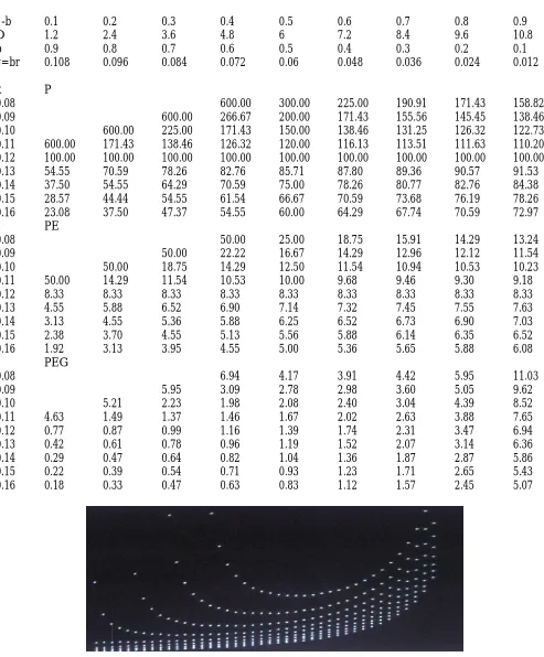
Fig. 1 Graphic of the PEG for discount rates .08 through .16
16) ∂PEG/∂b = (rb2 – 2rb +k)/(r3b4 – 2kr2b3+k2rb2) = 0
17) b2 – 2b +k/r = 0 and thus
18) b = (2 ± [4 – 4k/r]1/2)/2 = 1 ± (1-k/r)1/2
which indicates that a non monotonic minimum PEG per retention policy exists when k is less than r and which was observed. But is this appropriate policy for firms achieving returns greater than their discount rates? The users of the PEG cite its value as an optimum valuation when it is close to one. And to be fair, it does work poorly—but only for under performing firms but in no case is it is neither desirable nor feasible for over performing firms.
In contrast to the bizarre treatment that the PEG presents to the PE ratio, there exists a more straightforward one which is the payout ratio. It can be determined from available investment data. Consider generally found public data such as:
Company Div. Yield PE Vol. High Low Close Change
LMU 2.00 4.0 10 237 50.5 45.5 50.0 +.75
One could impute the firm’s earnings from the PE and the firm’s share price or here that the PE of 10 equals the price of 50 divided by earnings which here must be 5. Thus one could deduce that the payout ratio is D/E or here is 2/5 or 40 percent. But the PE ratio multiplied by the yield is a more direct approach noting that the PE times D/P cancels the price components or here 4.0 times 10 which equals again 40 percent. And the payout ratio is more indicative of a firm’s health in that low payout ratios are associated with riskier firms of both kinds—those that unhealthy per se and those which are more speculative in terms of being newer and/or more aggressive in regards to reinvestment policy. Likewise high payout ratios are more indicative of more staid firms albeit at the same time can portend a not so fortuitous future decline in dividends.Moreover, if one knows the PEG then one can determine the firm’s growth rate which here if the PEG was 1.67 then the growth rate must be 6 percent from g = PE/PEG. If one knows the firm’s growth rate, then one can infer the firm’s rate return to be achieved from g = br or here r = g/b. Thus, if one knew that the growth rate was 6 percent then since the payout ratio is 40 percent then the retention rate is 60 percent and therefore here the firm’s inferred rate of return expected to be achieved is 10 percent.
Independent of the payout ratio, one can also use the growth rate to determine the market’s risk adjusted discount rate for the firm from:
19) k = D/P + g
which here would be the yield of 4 percent plus the growth rate of 6 percent or 10 percent. And here since r equals k then this security is likely trading near book value which would involve a discussion of Modigliani-Miller proposition that dividends do not matter as shown in equation 13 (see Investopedia, Wikipedia, and Modigliani & Miller). Lest one think that this result is likely or invariable consider some other growth rates and other PEGs:
Price P 50 50 50
Dividends D 2 2 2
Yield D/P 4% 4% 4%
Price/Earnings PE 10 10 10
PEG PE/g 1.67 2 1
Earnings E = P/PE 5 5 5
Payout 1-b = D/E .4 .4 .4
= YieldxPE 40% 40% 40%
Retention b = 1-b 60% 60% 60%
Growth g = PE/PEG 6% 5% 10%
Return Achieved r = g/b 10% 8.3% 16.7%
Discount Rate k = D/P + g 10% 9% 14%
In conclusion, it seems that the PEG was an attempt to undo the growth component of the PE ratio which rises as growth increases. It would seem a more useful procedure to instead use the PE and PEG ratios in a more productive manner to directly determine the firm’s payout ratio and with the growth rate to infer the firm’s risk adjusted discount rate and the firm’s expected rate of return to be achieved.
References
Craine, Roger “Notes on Intrinsic Valuation Models” [2005]
http://eml.berkeley.edu/~craine/EconH195/Fall_14/webpage/Notes%20on%20the%20Gordon%20Valuation%20 Formula3.pdf
Farina, Mario A Beginner's Guide To Successful Investing In The Stock Market [1969]
Gordon, Myron "Dividends, Earnings and Stock Prices" Review of Economics and Statistics [1959] Investing Answers “How To Use the Gordon Growth Model”
http://www.investinganswers.com/education/stock-valuation/how-use-gordon-growth-model-2456 Investopedia “Modigliani-Miller Theorem – M&M”
http://www.investopedia.com/terms/m/modigliani-millertheorem.asp
Investopedia “Price/Earnings to Growth – PEG Ratio” http://www.investopedia.com/terms/p/pegratio.asp Lynch, Peter One Up on Wall Street [1989]
Modigliani, F.; Miller, M. [1958] "The Cost of Capital, Corporation Finance and the Theory of Investment"American
Economic Review48 (3), pp. 261–297.
Modigliani, F.; Miller, M. [1963] "Corporate income taxes and the cost of capital: a correction"American Economic
Review53 (3), pp. 433–443.
Wikipedia “Dividend Discount Model” http://en.wikipedia.org/wiki/Dividend_discount_model Wikipedia “Modligiani-Miller Theorem”