Int. J. Nonlinear Anal. Appl. 11 (2020) No. 1, 137-157 ISSN: 2008-6822 (electronic)
http://dx.doi.org/10.22075/ijnaa.2020.4245
Woodpecker Mating Algorithm (WMA): a
nature-inspired algorithm for solving optimization
problems
Morteza Karimzadeh Parizia, Farshid Keynia*b, Amid khatibi Bardsiria
a Department of Computer Engineering, Kerman Branch, Islamic Azad University, Kerman, Iran;
b Department of Energy Management and Optimization, Institute of Science and High Technology and Environmental
Sciences, Graduate University of Advanced Technology, Kerman, Iran;
(Communicated by J. Vahidi)
Abstract
Nature-inspired metaheuristic algorithms have been a topic of interest for researchers to solve op-timization problems in engineering designs and real-world applications, due to their simplicity and flexibility. This paper presents a new nature-inspired search algorithm called Woodpecker Mating Algorithm (WMA) and applies it to challenging problems in structural optimization. The WMA is a population-based metaheuristic algorithm that mimics the mating behavior of woodpeckers. It was inspired by the drumming sound intensity. In WMA, the population of woodpeckers is divided into male and female groups. The female woodpeckers approach the male woodpeckers based on the intensity of their drum sound. An efficiency comparison was drawn between the WMA algorithm and other metaheuristic algorithms by employing 19 benchmark functions(including unimodal, multi-modal and composite functions). Moreover, the performance of WMA is compared with 8 of the best meta-heuristic algorithms using 13 high dimensional multimodal and unimodal benchmark functions. The assessments and statistical results indicate that the WMA algorithm offers promising results and is capable of outperforming the most recent and popular algorithms proposed in the literature in most of the employed benchmark functions. Moreover, a statistically significant difference was observed compared to the other assessed algorithms. The proposed algorithm produced significant results for a non-convex, inseparable, and scalable problems.
∗Farshid Keynia
Email address: [email protected], [email protected], [email protected](Morteza Karimzadeh Parizia, Farshid Keynia*b, Amid khatibi Bardsiria)
138 Morteza Karimzadeh Parizi, Farshid Keynia, Amid khatibi Bardsiri
Keywords: Metaheuristic, Optimization, Woodpecker, Drumming, Sound intensity.
2010 MSC: 68T99,68W25,68T20.
1. Introduction
Optimization is the process of obtaining optimal values for the parameters of a specific system from all of the possible values to maximize or minimize its output. The optimization problem can be observed in all research fields because it has led to the development of optimization techniques and also the emergence of intriguing areas for researchers [1]. In the past two decades, there has been a growing interest in metaheuristic algorithms in order to solve the optimization problems[2]. Metaheuristic algorithms are popular because they regard a problem as a black box [1, 3]. They avoid the local optimum due to their random nature [2, 4]. Finally, they are easy to learn and implement [5, 6]. Since metaheuristic algorithms are mainly based on the regulations of natural organisms, they are
called nature inspired [7]. Depending on the nature of a simulated phenomenon, metaheuristic
algorithms can be categorized into four classes: evolutionary, physics-based, swarm intelligence and inspired by human behaviour [2].
The evolutionary algorithms (EA) are generally certain optimization algorithms inspired by the Darwinian principles of nature in relation to the abilities to live organisms to evolve and adapt to environmental conditions. For instance, Genetic Algorithm(GA) [8, 9], Differential Evolution (DE) [10], Evolutionary Programming (EP), Evolution Strategies (ES) [11], are evolutionary algorithms. The second class includes physics-based techniques. These optimization algorithms are usually the simulations of physical laws. For instance, they apply to motion, gravity, radiation, electromagnetic, weight, etc [5]. The instances are Multi-Verse Optimizer (MVO) [3], Simulated Annealing (SA) [12], Thermal Exchange Optimization (TEO) [13] and Orientation Search Algorithm (OSA) [14].
The third class of metaheuristic algorithms was inspired by human behaviour. The instances include Harmony Search (HS) [8, 15], Brain Storm Optimization Algorithm (BSOA) [16], Imperialist Com-petitive Algorithm (ICA) [17], Kidney-inspired algorithm (KA) [18], Interior Search Algorithm (ISA) [19], Single Seekers Society (SSS) [20], Sine Cosine Algorithm (SCA) [21], Poor and rich optimization algorithm (PRO) [22], group teaching optimization algorithm (GTOA) [23] and Teaching Learning Based Optimization (TLBO) [24].
The fourth class is called swarm intelligence (SI), which is a distributed intelligence model used to solve optimization problems. SI was inspired by the collective behaviour of a swarm of social insects and other animal swarms. SI is usually made up of a simple population of elements (an institution which is able to carry out certain operations) which operate with each other and the environment locally. With very limited capabilities, these institutions can cooperate to carry out very complicated tasks for survival [25]. Particle Swarm Optimization (PSO) [26, 27] , Artificial Bee Colony (ABC) [28], Ant Colony Optimization (ACO) [29], Satin Bowerbird Optimizer (SBO) [30], Dragonfly algorithm (DA) [31], Grey Wolf Optimizer (GWO) [5], Moth-flame Optimization (MFO) [32], Bat Algorithm (BA) [33], Firefly Algorithm (FA) [34], Cuckoo Search (CS) [35], Ant Lion Optimizer (ALO) [4], Whale Optimization Algorithm [2] ,Harris Hawks Optimizer (HHO) [36], Crow Search Algorithm (SCA) [37, 38], Donkey and Smuggler Optimization Algorithm (SDO) [39] and Artificial Acari Optimization (AAO) [40] are SI algorithms.
Woodpecker Mating Algorithm 11 (2020) No. 1, 137-157 139
It can be defined as the process of analyzing a promising area found in the exploration phase [2]. The exploitation phase emphasizes the local search, and the algorithm converges to the promising areas found in the exploration phase [3]. Exploration and exploitation are two opposite turning points. Promoting the results of one phase downgrades the results of the other. The proper balance between these two turning points can guarantee an accurate estimation of the global optimum by using population-based algorithms [32].
In this study, a novel nature-inspired metaheuristic algorithm was introduced based on the mating behavior of woodpeckers. Woodpeckers peck at trees (drumming) to attract the opposite sex. Pecking results in a sound wave. According to the physics laws, sound waves propagate in the environment so that other woodpeckers can hear them. Therefore, the physical quantity is defined as sound intensity, on which the amount of sound received by a listener depends. Such concepts provided the inspiration for the proposed algorithm.
The rest of this paper contains four sections. In Section 2, the woodpecker mating algorithm is
introduced. In Section3, mathematical benchmark functions are used to evaluate the proposed
algorithm. Finally, Section 4, presents the conclusion and suggestions for future studies.
2. Woodpecker Mating Algorithm (WMA)
Woodpeckers are wonderful birds. There are nearly 200 different species of them. Woodpeckers use a specific strategy for communication. It is called drumming or pecking the trunks of trees. Drumming gives provides woodpeckers with special opportunities. They make holes into the trunks of trees to build nests and feed on insects or resin. By doing so, they can also communicate with other woodpeckers, show their territories, and scare their enemies. However, the most important purpose of drumming is to attract mates in the mating season [43]. In fact, drumming is an intra-gender competition in the mating season. Male woodpeckers compete with each other to attract female birds by drumming. Before a female woodpecker selects a mate, it listens to multiple drumming sounds and analyzes them instinctively. Then it gets attracted to the sound with the highest quality and flies toward the source of drumming (the male woodpecker). The drumming rate differs in different species. It falls down in larger species, and they make louder phones instead. However, drumming is the main non-phonetic tool for long-distance communication. The WMA algorithm was inspired
by the mating behaviour of red-bellied woodpeckers (Melanerpes carolinus) [44]. In the proposed
algorithm, it is assumed that drumming is the only communication tool used by woodpeckers. At the beginning of the mating season, male woodpeckers start drumming. The quality of the sound produced by the male has a great effect on the attraction of female woodpeckers. Like other animals, woodpeckers try to attract and choose the best mate. Birds with the higher ability for drumming can produce stronger, higher quality drums and are regarded as ideal mates. Their drum can be heard farther away and attract more female woodpeckers. The female woodpeckers are then attracted to the source, because for them a more powerful sound connotes the male’s higher ability to find food, nest and reproduce, making them a better option as mate. As a result, the acoustic power
(sound intensity) of the male woodpecker’s drum indicates its ability to attract female birds. In other words, the size of a female woodpecker’s movement toward a male woodpecker depends on the quality of sound it hears. The stronger the sound, the closer the female woodpecker gets to the male bird producing it. It is worth noting that powerful or high quality sound means the physical quantity of ”sound intensity” as described below.
140 Morteza Karimzadeh Parizi, Farshid Keynia, Amid khatibi Bardsiri
these periodic drums attract the female bird step by step. This approach is similar to an evolutionary process, and by each iteration, the female woodpecker gets closer to the male. On the other hand, when a male woodpecker strikes a tree, the sound is transmitted to the environment and to the ears of other females, so they move toward the male bird. Since the basis of the movement is the position of the male bird, and the female woodpeckers move toward it based on the information obtained from processing the male bird’s drum, there is a process of communication and flow of information between the male and the female woodpeckers. So, this process is a swarm intelligence behavior.In the nature, at the beginning of the mating season, many male woodpeckers begin drumming to attract female woodpeckers as mates. As a result, at each time interval, a female woodpecker hears the drum sound of several males at the same time. As mentioned in the preceding paragraph, female woodpeckers look for the best males. But if another male (other than the best male) is closer to the female, the female bird will be attracted to this male because it will receive a better quality drum due to the shorter distance from the sound source.
2.1. Sound Intensity
In the physics of sound waves [45], the received sound depends on a quantity named the sound
intensity. The sound intensity (SI) of one level is the average energy changes reaching or exceeding
a level. It can be calculated through Equation (2.1):
SI = P
A (2.1)
In this equation, P is the sound power, and A is the area meeting the sound.
It is often complicated to determine how sound intensity changes over the distance from a real source of the sound. Some of the sources (such as speakers) may send out the sound only in one direction. The environment usually generates some echoes overlapping with the direct sound wave. However, the echoes can sometimes be ignored in some cases. It can be assumed that the source of sound is a point emitting the sound in an isotropic way, i.e. with the same intensity in all directions (This
assumption is true about woodpeckers.). In addition, the mechanical energy of sound waves (P) is
conserved when waves are spread from a source. If a sphere is assumed with a radius ofr around the
source, All the energy emitted by the source must pass through the surface of the sphere. Thus, the transfer rate of sound wave energy through the perimeter should be equal to the propagation rate of the source (PS). As a result, sound intensity (I) is defined as Equation (2.2):
SI = PS
4πr2 (2.2)
Here 4πr2is the area of the sphere. According to Equation (2.2), the sound intensity of an isotropic
point source decreases by the squared distance r2. Therefore, the intensity of the received sound
depends greatly on the distance between an object and the source. The shorter the distance is, the
higher and better the sound will be received. The Euclidean distance (r) can be calculated through
Equation (2.3):
r=kXS− X0k (2.3)
HereXSis the position of the sound-generating source, andX0 is the position of a listener.
So far, it has been assumed that female woodpeckers fly towards a male woodpecker based on sound
intensity(I). Other main factor is distance. Intensity of the received sound is depended on the
Woodpecker Mating Algorithm 11 (2020) No. 1, 137-157 141
2.2. The WMA algorithm assumptions
The WMA algorithm is inspired by the aforementioned concepts and based on the following assump-tions.
1. The only way of communication for the woodpeckers is the sound produced via drumming. 2. All female woodpeckers hear a percentage of the drum from most appropriate male per their distance and are attracted to it.
3. The fitness of a male woodpecker is calculated based on the objective function.
4. In the WMA algorithm, fitness is considered an attractiveness factor. Female woodpeckers are attracted to the more qualified male woodpeckers. The best woodpecker, also called the gpop. 5. The rate at which a female woodpecker is attracted to a male bird depends on the ”sound intensity” of the drum she hears. On the other hand, the rate of attraction, according to the laws of physics in terms of acoustic waves, decreases with increasing distance from the source. The smaller the distance, the greater the amount of attraction for a female woodpecker.
6. In the WMA, woodpecker populations are considered as male and female woodpeckers based on their level of fitness. The male woodpecker population is large at the beginning of exploration
(because at the beginning of the mating season the number of single males is high). But this
population decreases with the increase in the number of iterations of the algorithm (as the mating season advances, the number of single male birds declines, due to successful mating). This process leads to exploitation.
7. In early iterations (at the beginning of the mating season), female woodpeckers are attracted to the most appropriate and the least distant male woodpeckers. But in the later iterations, they are attracted only to the best woodpecker.
8. For the sake of simplification, it is assumed that, besides the gpop drum, each female woodpecker will hear only one other male woodpecker at any certain point of time, that is, the male which is the closest to the female bird, and therefore, has a higher drum sound intensity.
As mentioned above, WMA is a swarm intelligence algorithm that inspired on the mating behavior of woodpeckers. There are some similarities between the WMA and the Firefly Algorithm (FA) in scientific terms. But the two are very different from technical and operator aspects. In FA, the concept of light intensity is discussed as the amount of attraction of two fireflies, whereas in the WMA, the concept of sound intensity is used as a measure of the attraction of search agents. These two concepts are quite different in terms of physics laws and formulations. In FA, the population of fireflies are considered unisex, and each firefly can be attracted by a more fitting search agent. However, the woodpecker population in the WMA is considered as male and female woodpeckers. Each female woodpecker is attracted to the best (or the gpop) and the nearest male woodpecker. Unlike FA, the WMA algorithm has several operators for sequential and efficient implementation of exploration and exploitation phases that have a significant effect on WMA performance and its global and local search capability
2.3. Mathematical model and optimization algorithm
142 Morteza Karimzadeh Parizi, Farshid Keynia, Amid khatibi Bardsiri
fitness is selected as the best gpop. The gpop is the most attractive woodpecker, and all female woodpeckers hear a
percentage of its drum relative to their distance, and move toward it.
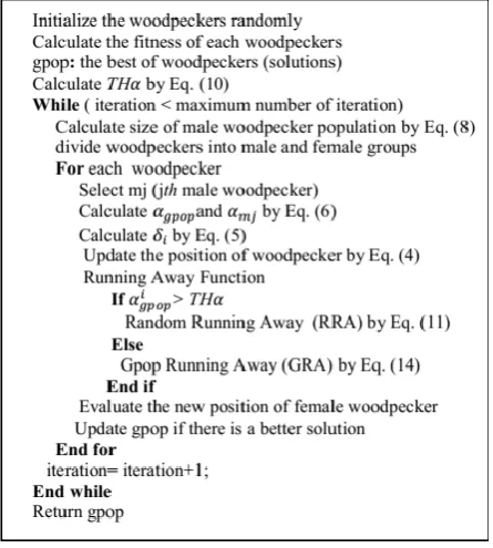
Fig. 1. Pseudo code of the WMA
2.3.3. Woodpeckers in Motion
In this step, every woodpecker updates its position through Equation (4).
(4) 𝑥𝑖𝑡+1= 𝑥𝑖𝑡+ 𝑟 ∗𝛿𝑖
𝑡∗(𝛼
𝑔𝑝𝑜𝑝∗(𝑥𝑔𝑝𝑜𝑝𝑡 −𝑥𝑖𝑡)+𝛼𝑚𝑗∗(𝑥𝑚𝑗𝑡 −𝑥𝑖𝑡))
2
Here 𝑥𝑖𝑡 indicates the previous position of the ith woodpecker, and 𝑥𝑔𝑝𝑜𝑝𝑡 shows the position of the best member (gpop, the
best male). Moreover, 𝑥𝑚𝑗𝑡 is the position of the jth male woodpecker, 𝑟 is a random number of a uniformly distribution
selected from [0, 1], 𝛿𝑖𝑡 shows the random coefficients for the i-th woodpecker in iteration t. The values of these coefficients
are calculated adaptively along the iteration cycle of the algorithm based on Equation (5). The 𝛼(𝛼𝑔𝑝𝑜𝑝, 𝛼𝑚𝑗 ) is a parameter
which can be determined through Equation (6(. In fact, 𝛼 indicates how much a woodpecker is attracted to a male
woodpecker (i.e. the target position) based on a ratio of the received sound intensity ( really 𝛼 determines the amount of
step).
As mentioned in the preceding section, a female woodpecker may, at each time slice of the mating season, be affected by and
attracted not only to the gpop but also to the drum sound of the closest male woodpecker. In equation (4) xmj is the indicator
of the position of this male. In fact, every female woodpecker updates its position based on gpop and a male woodpecker
selected as 𝑚𝑗. Regarding the selection of an𝑚𝑗from male birds, the Euclidean distance of a female woodpecker (i) from
every male bird is determined in each iteration through Equation (3). Then the male bird being on the shortest distance from
Figure 1: Pseudo code of the WMA
birds and update their position based on the location of male birds. If they find a better candidate solution, they will update the position of the male woodpecker.
2.3.1. Initialization
The WMA algorithm is a population-based algorithm. Here every woodpecker is considered a candi-date solution. Like other metaheuristic algorithms, the proposed algorithm initializes with a group of random woodpeckers ( random candidate solutions). In fact, woodpeckers are distributed uniformly
in the search space. Every woodpecker is an n-dimensional solution vector for the problem. Other
parameters of the algorithm such as maximum iteration, population size, RA probability, and sound wave power are adjusted in this step. Fig. 1 shows the pseudo code of the proposed WMA algorithm.
2.3.2. Evaluation and Divide Population of the Woodpeckers
Like other birds, woodpeckers tend to select the best mate. Thus, the better young woodpeckers can be born. In this step, the population of woodpeckers is evaluated by the objective function to determine their fitness values. Then the population of woodpeckers is divided into male and female groups. At the beginning of each iteration, the woodpecker population is sorted on the basis of the rate of fitness value according to the objective function, and proportional to the size of the male woodpecker population, the most qualified woodpeckers are considered to be male birds. In each iteration, male woodpeckers are search agents with the highest degree of fitness based on the objective function. The male with the highest degree of fitness is selected as the best gpop. The gpop is the most attractive woodpecker, and all female woodpeckers hear a percentage of its drum relative to their distance, and move toward it.
2.3.3. Woodpeckers in Motion
In this step, every woodpecker updates its position through Equation (2.4).
xti+1 =xti +r∗
δt i ∗
αgpop∗(xtgpop−xti) +αmj ∗(xtmj −xti)
Woodpecker Mating Algorithm 11 (2020) No. 1, 137-157 143
Here xti indicates the previous position of the ith woodpecker, and xtgpop shows the position of the
best member (gpop, the best male). Moreover,xt
mj is the position of the jth male woodpecker, ris a random number of a uniformly distribution selected from [0, 1], δt
i shows the random coefficients for
thei-th woodpecker in iterationt. The values of these coefficients are calculated adaptively along the iteration cycle of the algorithm based on Equation (2.5). The α(αgpop, αmj ) is a parameter which
can be determined through Equation (6(. In fact, α indicates how much a woodpecker is attracted
to a male woodpecker (i.e. the target position) based on a ratio of the received sound intensity (
really α determines the amount of step).
As mentioned in the preceding section, a female woodpecker may, at each time slice of the mating season, be affected by and attracted not only to the gpop but also to the drum sound of the closest
male woodpecker. In equation (2.4) xmj is the indicator of the position of this male. In fact,
every female woodpecker updates its position based on gpop and a male woodpecker selected as mj.
Regarding the selection of an mjfrom male birds, the Euclidean distance of a female woodpecker (i)
from every male bird is determined in each iteration through Equation (2.3). Then the male bird
being on the shortest distance from the female woodpecker will be selected as themj. In fact, gpop
shows the best male bird in the population. As a result, it generates the highest quality of drumming
sounds influencing the female woodpeckers. The male mj is near a female bird; thus, it pecks at
trees to influence the female bird and make it develop certain desires. Fig. 2 shows how a female
woodpecker updates its position according to gpop andmj in a 2D search space.
δti =r∗b (2.5)
In this equation, r is a random number from a uniform random distribution in [0, 3]. The value of
parameterb decreases from 0.77 to 0 during the iteration cycle of the algorithm. With this reduction,
the exploration and exploitation phases are respectively implemented efficiently. The value of b in
each iteration of the algorithm is calculated using equation (2.7).
δt
i has a random value in the range of [0, 3b] which decreases the value ofδti as well as its fluctuation range by decreasingb during the iteration cycle of the algorithm. If the value ofδitis in the range of [0, 1],the new position of a female woodpecker is placed at any random point between its current position and the target woodpecker’s position (gpop or mj). In other words, female woodpeckers converge and get closer to the target woodpecker. This practice emphasizes exploitation phase particularly on end iterations. In this case, search agents are required to search locally in promising areas around male woodpeckers in order to enhance the quality of the received solutions. On the other hand, if
δti>1, then female woodpeckers are required to far away the target woodpecker and diverge from it. This results in the exploration of new promising areas for better solutions. In this case, the WMA algorithm can search globally. In short, if δt
i ≤1, then the female woodpeckers have to converge to
the target woodpecker (Fig. 3a); otherwise, they have to diverge from it (Fig. 3b).
α= 1
1+SIij (2.6)
In this equation, α shows the probability (attraction) of male woodpecker j for woodpecker i
and SIij is the sound intensity of the target woodpecker (j), reaching female woodpecker i. In
fact, Parameter α are amount of the pace in relation to the attractiveness (sound intensity) of the
144 Morteza Karimzadeh Parizi, Farshid Keynia, Amid khatibi Bardsiri
the female woodpecker will be selected as the 𝑚𝑗. In fact, gpop shows the best male bird in the population. As a result, it
generates the highest quality of drumming sounds influencing the female woodpeckers. The male 𝑚𝑗 is near a female bird;
thus, it pecks at trees to influence the female bird and make it develop certain desires. Fig. 2 shows how a female woodpecker
updates its position according to gpop and 𝑚𝑗 in a 2D search space.
Fig. 2. Position updating in WMA Algorithm
(5) 𝛿𝑖𝑡= 𝑟 ∗ 𝑏
In this equation, r is a random number from a uniform random distribution in [0, 3]. The value of parameter b decreases from
0.77 to 0 during the iteration cycle of the algorithm. With this reduction, the exploration and exploitation phases are
respectively implemented efficiently. The value of b in each iteration of the algorithm is calculated using equation (7).
𝛿𝑖𝑡has a random value in the range of [0, 3b] which decreases the value of 𝛿𝑖𝑡 as well as its fluctuation range by decreasing b
during the iteration cycle of the algorithm. If the value of 𝛿𝑖𝑡 is in the range of [0, 1],the new position of a female woodpecker
is placed at any random point between its current position and the target woodpecker's position (gpop or mj). In other words,
Woodpecker Mating Algorithm 11 (2020) No. 1, 137-157 145
female woodpeckers converge and get closer to the target woodpecker. This practice emphasizes exploitation phase
particularly on end iterations. In this case, search agents are required to search locally in promising areas around male
woodpeckers in order to enhance the quality of the received solutions. On the other hand, if 𝛿𝑖𝑡>1, then female woodpeckers
are required to far away the target woodpecker and diverge from it. This results in the exploration of new promising areas for
better solutions. In this case, the WMA algorithm can search globally. In short, if 𝛿𝑖𝑡≤ 1, then the female woodpeckers have
to converge to the target woodpecker (Fig. 3a); otherwise, they have to diverge from it (Fig. 3b).
Fig. 3. illustrates the influence of the parameter 𝛿𝑖𝑡 on the next position of the female woodpecker.
(6) 𝛼 = 1
1+𝑆𝐼𝑗𝑖
In this equation, 𝛼 shows the probability (attraction) of male woodpecker j for woodpecker i and 𝑆𝐼𝑗𝑖 is the sound intensity of
the target woodpecker (j), reaching female woodpecker i. In fact, Parameter 𝛼 are amount of the pace in relation to the
attractiveness (sound intensity) of the selected male woodpecker. In fact, the pace is inversely related to the sound intensity.
In other words, the higher the sound intensity of a destination woodpecker is for female woodpecker, the greater the
denominator will be. Therefore, the pace will reduce. The pace is selected from (0, 1]. The greatest value is obtained when
the attractiveness of the destination woodpecker approaches zero (the received sound intensity is too low). The smaller the
pace is, the more accurately a woodpecker moves towards the destination. A woodpecker moves around the centralized
target, something which increases exploitation and results in a more accurate estimated optimal solution. Therefore,
parameter 𝛼 has an effect on the exploitation of the algorithm.
(7) 𝑏 = 𝑇𝑎𝑛𝑠𝑖𝑔 (1 − 𝑡
𝑡𝑚𝑎𝑥)
Figure 3: illustrates the influence of the parameterδt
i on the next position of the female woodpecker.
zero (the received sound intensity is too low). The smaller the pace is, the more accurately a
woodpecker moves towards the destination. A woodpecker moves around the centralized target, something which increases exploitation and results in a more accurate estimated optimal solution.
Therefore, parameter α has an effect on the exploitation of the algorithm.
b=T ansig
1− t
tmax
(2.7)
HereT ansig is the tangent sigmoid function, in which t is the current iteration number, andtmax is the maximum number of iterations.
The population of male woodpeckers decreases during the algorithm iteration cycle adaptively. In the final iterations, only one male woodpecker will remain. The large number of male woodpeckers can increase exploration in the initial iterations. Moreover, the algorithm is prevented from being trapped in local optimums. In the final iterations, decreasing the number of male birds increases
exploitation and accuracy of solutions. Equation (8(can be used for determining the number of male
woodpeckers in each iteration.
M alenu=
Round
N
2 ∗
1− t
tmax
+ 1
(2.8)
Here M alenu is the number of male woodpeckers in each iteration, and t is the current iteration
number. Moreover, tmax shows the maximum number of iterations, when N indicate the maximum
number of woodpeckers population.
As mentioned earlier, the population of male woodpeckers in the iteration cycle of the algorithm decreases linearly with increase of iterations. The minimum population for male woodpeckers is one woodpecker and that is the gpop. In this case, equation (2.4) is simplified as equation (2.9).
xti+1 =xti+r∗(δti∗(xtgpop−xti)∗αgpop) (2.9)
2.3.4. Running Away Function
146 Morteza Karimzadeh Parizi, Farshid Keynia, Amid khatibi Bardsiri
and deviates. On the other hand, a woodpecker might be attacked by other woodpeckers or hunting birds on the path. It may also make random changes to the path due to feeling danger. Such random changes are stimulated as Running Away (RA) function. In other words, path changes are regarded as random changes in the solutions. How the female woodpecker escapes can vary depending on the sound intensity it receives from the best member (gpop) of the population. In this section, two types of movement are considered as escape of woodpeckers. The criterion for selecting the type of
movement is based on the sound intensity threshold received from the gpop (THα). The value of
Hα is calculated by equation (2.11). Based on what was stated in the previous section, the value of
Hαis inversely related to the sound intensity. The larger the value ofαi
gpop, the greater the distance between the woodpecker and the gpop and the lower the quality of the drum. If αigpop> Hα, it is assumed that the woodpecker is far from the gpop and that the drum will be received with a very low sound intensity. In this case, the female woodpecker is at an inappropriate point relative to the gpop position, so it flies quite randomly based on the equation (2.10) to another point of search space (forest). This movement is called Random Running Away (RRA).
T Hα= 0.8∗
Pn−1
1 αigpop
n−1 (2.10)
in which Hα is the threshold for the gpop sound intensity that is calculated in the first iteration, n is size of the woodpeckers depart from, andαi
gpopis calculated proportional to the sound intensity of the woodpecker i, whose value is calculated using equation (2.6).
xiRRA=lb−(lb−ub)∗r (2.11)
In this equation,xi
RRAis the position of a new element obtained from RRA on theith woodpecker,
ris a random number of a uniformly continuous distribution selected from [0, 1]. lband ub are lower
and upper boundaries of variables Respectively. If αi
gpop< Hα, then the woodpecker has heard the sound of the gpop drums with acceptable sound
intensity. Therefore, it is in an appropriate position. In this situation, the woodpecker escapes to the gpop. This escape to gpop is called GRA (Gpop Running Away). The GRA rate is controlled
by the RA probability (PGRA).The values of PGRA decrease adaptively from γ to 0 in the algorithm
iteration cycle through Equation (2.12).
PGRA =γ∗( 1−
t tmax
) (2.12)
Here t is the current iteration number. Moreover, tmax shows the maximum number of iterations,
when γ indicate is RA coefficient.
In the proposed algorithm, GRA is performed with two parents. GRAbit is a vector as long as the
problem dimensions, the elements of which are obtained through Equation (2.13).
GRAbit =
1 if r ≤ PGRA
0 else (2.13)
In this equation, r is the jth element of the vector (as long as the problem dimensions). Every
element is a random number of uniform distribution, selected from [0, 1]. In the WMA algorithm, GRA is done according to Equation (2.14).
In the GRA operator, the female woodpecker escapes to the gpop. Another influential factor here
is the location of the random woodpecker (xr). This woodpecker is randomly selected from the
Woodpecker Mating Algorithm 11 (2020) No. 1, 137-157 147
fact, the female woodpecker escapes to the best male (gpop) and the position of a random woodpecker. The new position of the female woodpecker sits at any random point between the gpop positions and the random woodpecker.
xiGRA =xti+GRAbit∗
xtgpop−xr
∗R (2.14)
In this equation,xi
GRA is the position of a new element obtained from RA on theith woodpecker, and
xr is the position of a random woodpecker. Moreover, xtgpop shows the position of the best member
(gpop, the best male) int iteration. xti is the new position of theith woodpecker in iterationt, It was
obtained by moving in the search space in the previous step. R is a random number of a uniformly
distribution selected from [-1, 1]. t is the current iteration number. Every element of GRAbit vector with a value of one changes in the second expression of Equation (2.14).
At the end of this operator (Running away function), the fitness of xi
GRA or xiRRA is calculated by using the objective function. If the fitness value is better than xt
i, then it is replaces. Otherwise, the element that were generated by the RA operator will be ignored.
Given theHα value and the values larger thanα in the initial iterations in the WMA algorithm life
cycle, the RRA occurrence rate is higher in these iterations. Since in the RRA, female woodpeckers fly quite randomly around the search space, it results in exploration. As the algorithm cycle is repeated more and more, due to the approach of female woodpeckers to the gpop, as well as the declining
rate of α, the RRA rate decreases, and the GRA rate increases. At GRA operator, the random
movement of female woodpeckers around the gpop and another random woodpecker also increases
exploration. Although this random motion decreases with decreasingPGRAduring the iteration cycle
of the algorithm, it can still avoid stagnation in local optimality in the end iterations. By reducing
PGRA, due to the need to exploitation on the end iterations, the female woodpecker becomes more
concentrated on its position, leading to exploitation. In summary, the Running Away function has a great effect on the implementation of exploration in the initial iterations and in preventing recession in the local optimal.
2.3.5. Evaluating the new position and checking terminating conditions
In this step, the new position of the ith woodpecker is compared with the previous position and
the position of the best woodpecker. If the position is better than one, it will get replaced. If the termination condition of the algorithm is met, the best solution will be selected as the optimal solution to the problem. Otherwise, steps 3-5 are repeated.
3. Evaluation WMA algorithm by Benchmark Functions
148 Morteza Karimzadeh Parizi, Farshid Keynia, Amid khatibi Bardsiri
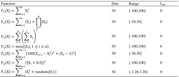
Table 1: Unimodal benchmark functions
very complicated because there are many local optimums, and different areas of the search space are in different forms. In
such functions, an optimization algorithm should strike an efficient balance between exploration and exploitation so that it
can move towards the global optimum. Thus, the main task of these functions is to evaluate exploration and exploitation
simultaneously [4, 46].
Table 1 Unimodal benchmark functions
fmin Range Dim Function 0 [-100,100] 30
F1(X) = ∑ Xi2 n
i=1
0 [-10,10]
30
F2(X) = ∑ |Xi| n i=1 + ∏|Xi| n i=1 0 [-100,100] 30
F3(X) = ∑ (∑ Xj i j−1 ) 2 n i=1 0 [-100,100] 30
F4(X) = max{|Xi|, 1 ≤ i ≤ n}
0 [-30,30]
30
F5(X) = ∑ [100(Xi+1− Xi2)2+ (Xi− 1)2] n−1
i=1
0 [-100,100]
30
F6(X) = ∑n ([Xi+ 0.5])2 i=1
0 [-1.28,1.28] 30
F7(X) = ∑ iXi4 n
i=1
+ random[0,1)
Table 2 Multimodal benchmark functions
fmin Range Dim Function -418*Dim [-500,500] 30
F8(X) = ∑ −Xi n
i=1 sin (√|Xi |)
0 [-5.12,5.12] 30
F9(X) = ∑n [Xi2− 10 cos(2πXi) + 10] i=1
0 [-32,32]
30
F10(X) = −20exp (−0.2√1 n∑ Xi2
n
i=1
) − exp (1
n∑ cos(2πXi) n
i=1
) + 20 + e
0 [-600,600] 30
F11(x) = 1
4000∑ Xi2 n
i=1
− ∏ cosXi √i n i=1 + 1 0 [-50,50] 30
F12(X) =π
n{10 sin(πy1) + ∑ (yi− 1)
2[1 + 10sin2(πyi+1)] n−1
i=1
+ (yn− 1)2} + ∑n u(Xi, 10,100,4) i=1
yi= 1 +Xi+ 1 4
u(Xi, a, k, m) = {
k(Xi− a)m xi> 𝑎 0 − a < xi< 𝑎
k(−Xi− a)mxi< 𝑎
0 [-50,50]
30
F13(x) = 0.1 {sin2(3πx1) + ∑n (xi− 1)2 i=1
[1 + sin2(3πxi+ 1)] + (xn− 1)2[1 + sin2(2πxn)]}
+ ∑ u(Xi, 5,100,4) n
i=1
.
The proposed algorithm was compared to a group of new and well-known metaheuristic algorithms such as Genetic
Algorithm (GA), Particle Swarm Optimization (PSO), Firefly Algorithm (FA) [8], Satin Bowerbird Optimizer (SBO) [30],
Artificial Bee Colony (ABC) [47], Wolf Optimizer (GWO) [5], Multi-Verse Optimizer (MVO) [3] and Bat Algorithm (BA)
[33].
All of the tests were run in MATLAB 2017a. Every benchmark function was run 30 times by the optimization algorithms.
The best results of 30 executions were calculated to compare the average (Ave) and standard deviation (Std). Then the
Wilcoxon signed rank test was employed to analyze the significance difference between the WMA and other algorithms. The
output was the statistical p_value. In this study, the significance level was considered 0.05; therefore, if the results of two
algorithms are lower than 0.05, they are statistically different. In all algorithms, the size of the initial population was 50, and
Table 2: Multimodal benchmark functions
very complicated because there are many local optimums, and different areas of the search space are in different forms. In
such functions, an optimization algorithm should strike an efficient balance between exploration and exploitation so that it
can move towards the global optimum. Thus, the main task of these functions is to evaluate exploration and exploitation
simultaneously [4, 46].
Table 1 Unimodal benchmark functions
fmin Range Dim Function 0 [-100,100] 30
F1(X) = ∑ Xi2 n
i=1
0 [-10,10]
30
F2(X) = ∑ |Xi| n
i=1
+ ∏|Xi| n
i=1
0 [-100,100] 30
F3(X) = ∑ (∑ Xj i j−1 ) 2 n i=1 0 [-100,100] 30
F4(X) = max{|Xi|, 1 ≤ i ≤ n}
0 [-30,30]
30
F5(X) = ∑ [100(Xi+1− Xi2)2+ (Xi− 1)2] n−1
i=1
0 [-100,100] 30
F6(X) = ∑ ([Xi+ 0.5])2 n
i=1
0 [-1.28,1.28] 30
F7(X) = ∑ iXi4 n
i=1
+ random[0,1)
Table 2 Multimodal benchmark functions
fmin Range Dim Function -418*Dim [-500,500] 30
F8(X) = ∑ −Xi n
i=1
sin (√|Xi|)
0 [-5.12,5.12] 30
F9(X) = ∑ [Xi2− 10 cos(2πXi) + 10] n
i=1
0 [-32,32] 30
F10(X) = −20exp (−0.2√ 1 n∑ Xi
2 n
i=1
) − exp (1
n∑ cos(2πXi) n
i=1
) + 20 + e
0 [-600,600] 30
F11(x) = 1 4000∑ Xi2
n
i=1 − ∏ cos Xi √i n
i=1 + 1
0 [-50,50] 30
F12(X) = π
n{10 sin(πy1) + ∑ (yi− 1)2[1 + 10sin2(πyi+1)] n−1
i=1
+ (yn− 1)2} + ∑ u(Xi, 10,100,4) n
i=1 yi= 1 +
Xi+ 1 4
u(Xi, a, k, m) = {
k(Xi− a)m xi> 𝑎 0 − a < xi< 𝑎
k(−Xi− a)mxi< 𝑎
0 [-50,50] 30
F13(x) = 0.1 {sin2(3πx1) + ∑ (xi− 1)2 n
i=1 [1 + sin
2(3πx
i+ 1)] + (xn− 1)2[1 + sin2(2πxn)]}
+ ∑ u(Xi, 5,100,4) n
i=1 .
The proposed algorithm was compared to a group of new and well-known metaheuristic algorithms such as Genetic
Algorithm (GA), Particle Swarm Optimization (PSO), Firefly Algorithm (FA) [8], Satin Bowerbird Optimizer (SBO) [30],
Artificial Bee Colony (ABC) [47], Wolf Optimizer (GWO) [5], Multi-Verse Optimizer (MVO) [3] and Bat Algorithm (BA)
[33].
All of the tests were run in MATLAB 2017a. Every benchmark function was run 30 times by the optimization algorithms.
The best results of 30 executions were calculated to compare the average (Ave) and standard deviation (Std). Then the
Wilcoxon signed rank test was employed to analyze the significance difference between the WMA and other algorithms. The
output was the statistical p_value. In this study, the significance level was considered 0.05; therefore, if the results of two
algorithms are lower than 0.05, they are statistically different. In all algorithms, the size of the initial population was 50, and between exploration and exploitation so that it can move towards the global optimum. Thus, the main task of these functions is to evaluate exploration and exploitation simultaneously [4, 46]. The proposed algorithm was compared to a group of new and well-known metaheuristic algorithms such as Genetic Algorithm (GA), Particle Swarm Optimization (PSO), Firefly Algorithm (FA) [8], Satin Bowerbird Optimizer (SBO) [30], Artificial Bee Colony (ABC) [47], Wolf Optimizer (GWO) [5], Multi-Verse Optimizer (MVO) [3] and Bat Algorithm (BA) [33].
All of the tests were run in MATLAB 2017a. Every benchmark function was run 30 times by the optimization algorithms. The best results of 30 executions were calculated to compare the average (Ave) and standard deviation (Std). Then the Wilcoxon signed rank test was employed to analyze the significance difference between the WMA and other algorithms. The output was the statistical p value. In this study, the significance level was considered 0.05; therefore, if the results of two algorithms are lower than 0.05, they are statistically different. In all algorithms, the size of the initial population was 50, and the maximum iteration was 500. The dimension of the problem (the number of decision-making variables) was 30. Table 4 shows the other parameters setting for each algorithm.
3.1. Evaluation of exploitation capability (functions F1-F7)
Woodpecker Mating Algorithm 11 (2020) No. 1, 137-157 149
Table 3: Composite benchmark functions
the maximum iteration was 500. The dimension of the problem (the number of decision-making variables) was 30. Table 4
shows the other parameters setting for each algorithm.
Table 3 Composite benchmark functions
fmin Range Dim Function 0 [-5,5] 10
F14(CF1)
𝑓1, 𝑓2, 𝑓3, … , 𝑓10= 𝑆𝑝ℎ𝑒𝑟𝑒𝐹𝑢𝑛𝑐𝑡𝑖𝑜𝑛
[ Ϭ1, Ϭ2, Ϭ3, … , Ϭ10] = [1, 1, 1, … , 1]
[ 𝜆1, 𝜆2, 𝜆3, … , 𝜆10] = [5/100, 5/100, 5/100, … , 5/100]
0 [-5,5] 10
F15(CF2)
𝑓1, 𝑓2, 𝑓3, … , 𝑓10= 𝐺𝑟𝑖𝑒𝑤𝑎𝑛𝑘′𝑠𝐹𝑢𝑛𝑐𝑡𝑖𝑜𝑛
[ Ϭ1, Ϭ2, Ϭ3, … , Ϭ10] = [1, 1, 1, … , 1]
[ 𝜆1, 𝜆2, 𝜆3, … , 𝜆10] = [5/100, 5/100, 5/100, … , 5/100]
0 [-5,5] 10
F16(CF3)
𝑓1, 𝑓2, 𝑓3, … , 𝑓10= 𝐺𝑟𝑖𝑒𝑤𝑎𝑛𝑘′𝑠𝐹𝑢𝑛𝑐𝑡𝑖𝑜𝑛
[ Ϭ1, Ϭ2, Ϭ3, … , Ϭ10] = [1, 1, 1, … , 1]
[ 𝜆1, 𝜆2, 𝜆3, … , 𝜆10] = [1, 1, 1, … , 1]
0 [-5,5] 10
F17(CF4)
𝑓1, 𝑓2= 𝑅𝑎𝑠𝑡𝑟𝑖𝑔𝑖𝑛′𝑠𝐹𝑢𝑛𝑐𝑡𝑖𝑜𝑛, 𝑓3, 𝑓4= 𝑊𝑒𝑖𝑒𝑟𝑠𝑡𝑟𝑎𝑠𝑠𝐹𝑢𝑛𝑐𝑡𝑖𝑜𝑛, 𝑓5, 𝑓6= 𝐺𝑟𝑖𝑒𝑤𝑎𝑛𝑘′𝑠𝐹𝑢𝑛𝑐𝑡𝑖𝑜𝑛
𝑓7, 𝑓8= Ackley′s Function, 𝑓9, 𝑓10= 𝑆𝑝ℎ𝑒𝑟𝑒𝐹𝑢𝑛𝑐𝑡𝑖𝑜𝑛
[ Ϭ1, Ϭ2, Ϭ3, … , Ϭ10] = [1, 1, 1, … , 1]
[ λ1,λ2,λ3, …,λ10]=[5/32, 5/32, 1, 1, 5/0.5, 5/0.5, 5/100, 5/100, 5/100, 5/100 ]
0 [-5,5] 10
F18(CF5)
𝑓1, 𝑓2= 𝑅𝑎𝑠𝑡𝑟𝑖𝑔𝑖𝑛′𝑠𝐹𝑢𝑛𝑐𝑡𝑖𝑜𝑛, 𝑓3, 𝑓4= 𝑊𝑒𝑖𝑒𝑟𝑠𝑡𝑟𝑎𝑠𝑠𝐹𝑢𝑛𝑐𝑡𝑖𝑜𝑛, 𝑓5, 𝑓6= 𝐺𝑟𝑖𝑒𝑤𝑎𝑛𝑘′𝑠𝐹𝑢𝑛𝑐𝑡𝑖𝑜𝑛
𝑓7, 𝑓8= Ackley′s Function, 𝑓9, 𝑓10= 𝑆𝑝ℎ𝑒𝑟𝑒𝐹𝑢𝑛𝑐𝑡𝑖𝑜𝑛
[ Ϭ1, Ϭ2, Ϭ3, … , Ϭ10] = [1, 1, 1, … , 1]
[ λ1,λ2,λ3, …,λ10]=[1/5, 1/5, 5/0.5, 5/0.5, 5/100, 5/100, 5/32, 5/32, 5/100, 5/100 ]
0 [-5,5] 10
F19(CF6)
𝑓1, 𝑓2= 𝑅𝑎𝑠𝑡𝑟𝑖𝑔𝑖𝑛′𝑠𝐹𝑢𝑛𝑐𝑡𝑖𝑜𝑛, 𝑓3, 𝑓4= 𝑊𝑒𝑖𝑒𝑟𝑠𝑡𝑟𝑎𝑠𝑠𝐹𝑢𝑛𝑐𝑡𝑖𝑜𝑛, 𝑓5, 𝑓6= 𝐺𝑟𝑖𝑒𝑤𝑎𝑛𝑘′𝑠𝐹𝑢𝑛𝑐𝑡𝑖𝑜𝑛
𝑓7, 𝑓8= Ackley′s Function, 𝑓9, 𝑓10= 𝑆𝑝ℎ𝑒𝑟𝑒𝐹𝑢𝑛𝑐𝑡𝑖𝑜𝑛
[ Ϭ1, Ϭ2, Ϭ3, … , Ϭ10]=[0.1, 0.2, 0.3, 0.4, 0.5, 0.6, 0.7, 0.8, 0.9, 1 ]
[ λ1,λ2,λ3, …,λ10]=[0.1 * 1/5, 0.2 * 1/5, 0.3 * 5/0.5, 0.4 * 5/0.5, 0.5 * 5/100,
0.6 * 5/100, 0.7 * 5/32, 0.8 * 5/32, 0.9 * 5/100, 1 * 5/100]
Table 4 Algorithm Parameters setting Parameters
Algorithm
Limit=100 ABC
roulette wheel selection, single point crossover with a crossover probability of 0.9, mutation probability of 0.01
GA
=0.94, z=0.02, mutation probability= 0.05
SBO
0=1, [0,1], =1 FA
c1=2, c2=2, ω=1
PSO
A=1, r=0.5, 𝑄𝑚𝑖𝑛=0, 𝑄𝑚𝑎𝑥=2, =0.99 , =0.01
BA
Ps=1, 𝛾 = 0.2
WMA
3.1. Evaluation of exploitation capability (functions F1-F7)
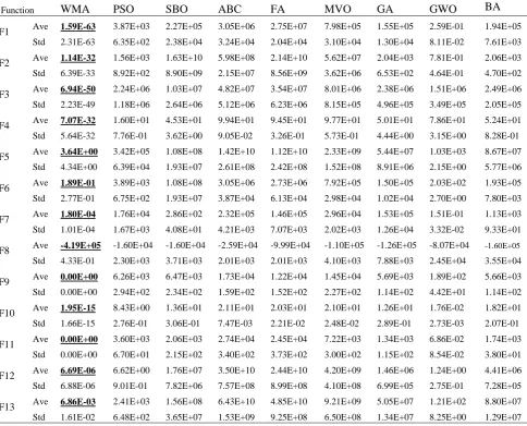
Table 5 shows the results of executing unimodal benchmark functions in optimization algorithms. Accordingly, the WMA
algorithm showed a better performance in 6 out of 7 unimodal functions than other algorithms. Given the features of these
functions, the results indicate the ability to highly exploit the proposed algorithm. Fig. 4 shows the convergence curve of
optimization algorithms in the unimodal functions. According to Fig. 4, the WMA performed the convergence process faster
than other algorithms in addition to a higher exploitability. The P-values of the Wilcoxon signed rank test can be seen in
Table 6. Accordingly, all of the p-values were smaller than 0.05. Therefore, there was a significant difference between the
WMA algorithm and other algorithms.
Table 4: Algorithm Parameters setting
the maximum iteration was 500. The dimension of the problem (the number of decision-making variables) was 30. Table 4
shows the other parameters setting for each algorithm.
Table 3 Composite benchmark functions
fmin Range Dim Function 0 [-5,5] 10
F24(CF1)
𝑓1, 𝑓2, 𝑓3, … , 𝑓10= 𝑆𝑝ℎ𝑒𝑟𝑒𝐹𝑢𝑛𝑐𝑡𝑖𝑜𝑛
[ Ϭ1, Ϭ2, Ϭ3, … , Ϭ10] = [1, 1, 1, … , 1]
[ 𝜆1, 𝜆2, 𝜆3, … , 𝜆10] = [5/100, 5/100, 5/100, … , 5/100]
0 [-5,5] 10
F25(CF2)
𝑓1, 𝑓2, 𝑓3, … , 𝑓10= 𝐺𝑟𝑖𝑒𝑤𝑎𝑛𝑘′𝑠𝐹𝑢𝑛𝑐𝑡𝑖𝑜𝑛
[ Ϭ1, Ϭ2, Ϭ3, … , Ϭ10] = [1, 1, 1, … , 1]
[ 𝜆1, 𝜆2, 𝜆3, … , 𝜆10] = [5/100, 5/100, 5/100, … , 5/100]
0 [-5,5] 10
F26(CF3)
𝑓1, 𝑓2, 𝑓3, … , 𝑓10= 𝐺𝑟𝑖𝑒𝑤𝑎𝑛𝑘′𝑠𝐹𝑢𝑛𝑐𝑡𝑖𝑜𝑛
[ Ϭ1, Ϭ2, Ϭ3, … , Ϭ10] = [1, 1, 1, … , 1]
[ 𝜆1, 𝜆2, 𝜆3, … , 𝜆10] = [1, 1, 1, … , 1]
0 [-5,5] 10
F27(CF4)
𝑓1, 𝑓2= 𝑅𝑎𝑠𝑡𝑟𝑖𝑔𝑖𝑛′𝑠𝐹𝑢𝑛𝑐𝑡𝑖𝑜𝑛, 𝑓3, 𝑓4= 𝑊𝑒𝑖𝑒𝑟𝑠𝑡𝑟𝑎𝑠𝑠𝐹𝑢𝑛𝑐𝑡𝑖𝑜𝑛, 𝑓5, 𝑓6= 𝐺𝑟𝑖𝑒𝑤𝑎𝑛𝑘′𝑠𝐹𝑢𝑛𝑐𝑡𝑖𝑜𝑛
𝑓7, 𝑓8= Ackley′s Function, 𝑓9, 𝑓10= 𝑆𝑝ℎ𝑒𝑟𝑒𝐹𝑢𝑛𝑐𝑡𝑖𝑜𝑛
[ Ϭ1, Ϭ2, Ϭ3, … , Ϭ10] = [1, 1, 1, … , 1]
[ λ1,λ2,λ3, …,λ10]=[5/32, 5/32, 1, 1, 5/0.5, 5/0.5, 5/100, 5/100, 5/100, 5/100 ]
0 [-5,5] 10
F28(CF5)
𝑓1, 𝑓2= 𝑅𝑎𝑠𝑡𝑟𝑖𝑔𝑖𝑛′𝑠𝐹𝑢𝑛𝑐𝑡𝑖𝑜𝑛, 𝑓3, 𝑓4= 𝑊𝑒𝑖𝑒𝑟𝑠𝑡𝑟𝑎𝑠𝑠𝐹𝑢𝑛𝑐𝑡𝑖𝑜𝑛, 𝑓5, 𝑓6= 𝐺𝑟𝑖𝑒𝑤𝑎𝑛𝑘′𝑠𝐹𝑢𝑛𝑐𝑡𝑖𝑜𝑛
𝑓7, 𝑓8= Ackley′s Function, 𝑓9, 𝑓10= 𝑆𝑝ℎ𝑒𝑟𝑒𝐹𝑢𝑛𝑐𝑡𝑖𝑜𝑛
[ Ϭ1, Ϭ2, Ϭ3, … , Ϭ10] = [1, 1, 1, … , 1]
[ λ1,λ2,λ3, …,λ10]=[1/5, 1/5, 5/0.5, 5/0.5, 5/100, 5/100, 5/32, 5/32, 5/100, 5/100 ]
0 [-5,5] 10
F29(CF6)
𝑓1, 𝑓2= 𝑅𝑎𝑠𝑡𝑟𝑖𝑔𝑖𝑛′𝑠𝐹𝑢𝑛𝑐𝑡𝑖𝑜𝑛, 𝑓3, 𝑓4= 𝑊𝑒𝑖𝑒𝑟𝑠𝑡𝑟𝑎𝑠𝑠𝐹𝑢𝑛𝑐𝑡𝑖𝑜𝑛, 𝑓5, 𝑓6= 𝐺𝑟𝑖𝑒𝑤𝑎𝑛𝑘′𝑠𝐹𝑢𝑛𝑐𝑡𝑖𝑜𝑛
𝑓7, 𝑓8= Ackley′s Function, 𝑓9, 𝑓10= 𝑆𝑝ℎ𝑒𝑟𝑒𝐹𝑢𝑛𝑐𝑡𝑖𝑜𝑛
[ Ϭ1, Ϭ2, Ϭ3, … , Ϭ10]=[0.1, 0.2, 0.3, 0.4, 0.5, 0.6, 0.7, 0.8, 0.9, 1 ]
[ λ1,λ2,λ3, …,λ10]=[0.1 * 1/5, 0.2 * 1/5, 0.3 * 5/0.5, 0.4 * 5/0.5, 0.5 * 5/100, 0.6 * 5/100, 0.7 * 5/32, 0.8 * 5/32, 0.9 * 5/100, 1 * 5/100]
Table 4 Algorithm Parameters setting Parameters
Algorithm
Limit=100 ABC
roulette wheel selection, single point crossover with a crossover probability of 0.9, mutation probability of 0.01
GA
=0.94, z=0.02, mutation probability= 0.05
SBO
0=1, [0,1], =1 FA
c1=2, c2=2, ω=1
PSO
A=1, r=0.5, 𝑄𝑚𝑖𝑛=0, 𝑄𝑚𝑎𝑥=2, =0.99 , =0.01
BA
Ps=1, 𝛾 = 0.2
WMA
3.1. Evaluation of exploitation capability (functions F1-F7)
Table 5 shows the results of executing unimodal benchmark functions in optimization algorithms. Accordingly, the WMA
algorithm showed a better performance in 6 out of 7 unimodal functions than other algorithms. Given the features of these
functions, the results indicate the ability to highly exploit the proposed algorithm. Fig. 4 shows the convergence curve of
optimization algorithms in the unimodal functions. According to Fig. 4, the WMA performed the convergence process faster
than other algorithms in addition to a higher exploitability. The P-values of the Wilcoxon signed rank test can be seen in
Table 6. Accordingly, all of the p-values were smaller than 0.05. Therefore, there was a significant difference between the
150 Morteza Karimzadeh Parizi, Farshid Keynia, Amid khatibi Bardsiri
Table 5: Results of unimodal benchmark functions
Table 5 Results of unimodal benchmark functions
Function WMA PSO SBO ABC FA MVO GA GWO BA
F1 Ave 1.75E-67 5.43E-06 8.43E-02 5.90E+03 1.61E+04 1.23E+00 2.48E+00 1.07E-27 3.46E+03
Std 2.35E-67 2.59E-05 2.88E-02 1.01E+03 3.79E+03 3.76E-01 1.16E+00 1.56E-27 9.62E+02
F2 Ave 1.03E-34 4.91E-03 1.08E-01 6.42E+01 1.23E+02 3.92E+00 3.43E-01 9.20E-17 8.41E+05
Std 6.91E-35 5.13E-03 2.47E-02 5.47E+00 9.52E+01 1.63E+01 8.23E-02 7.08E-17 3.08E+06
F3 Ave 4.26E-59 6.53E+02 9.57E+02 4.17E+04 2.37E+04 2.07E+02 4.35E+03 5.81E-06 9.89E+03
Std 1.41E-58 1.12E+03 2.85E+02 4.74E+03 6.98E+03 7.65E+01 1.72E+03 7.35E-06 3.44E+03
F4 Ave 5.52E-34 4.17E-01 1.73E+00 7.04E+01 8.55E+06 2.37E+00 7.61E+00 7.27E-07 2.41E+01
Std 4.72E-34 1.54E-01 1.07E+00 4.81E+00 3.64E+06 1.08E+00 1.33E+00 7.27E-07 5.53E+00
F5 Ave 3.87E+00 3.57E+01 2.58E+02 1.56E+07 8.55E+06 3.80E+02 2.73E+02 2.69E+01 5.63E+05
Std 9.51E+00 2.53E+01 3.50E+02 2.59E+06 3.64E+06 6.25E+02 1.42E+02 8.64E-01 3.16E+05
F6 Ave 5.46E-03 3.81E-07 9.73E-02 6.25E+03 1.64E+04 1.36E+00 2.35E+00 7.78E-01 3.42E+03
Std 3.91E-03 5.71E-07 3.37E-02 9.87E+02 3.33E+03 3.71E-01 8.43E-01 3.33E-01 1.42E+03
F7 Ave 8.96E-05 8.90E-02 1.57E-01 7.32E+00 2.52E+00 3.46E-02 1.08E-01 2.06E-03 5.91E-01
Std 7.58E-05 2.84E-02 3.66E-02 1.65E+00 8.50E-01 1.46E-02 4.19E-02 8.29E-04 3.73E-01
Table 6 P-values obtained from unimodal benchmark functions
Function PSO SBO ABC FA MVO GA GWO BA
F1 1.73E-06 1.73E-06 1.73E-06 1.73E-06 1.73E-06 1.73E-06 1.73E-06 1.73E-06
F2 1.73E-06 1.73E-06 1.73E-06 1.73E-06 1.73E-06 1.73E-06 1.73E-06 1.73E-06
F3 1.73E-06 1.73E-06 1.73E-06 1.73E-06 1.73E-06 1.73E-06 1.73E-06 1.73E-06
F4 1.73E-06 1.73E-06 1.73E-06 1.73E-06 1.73E-06 1.73E-06 1.73E-06 1.73E-06
F5 1.73E-06 1.73E-06 1.73E-06 1.73E-06 1.73E-06 1.73E-06 4.45E-05 1.73E-06
F6 1.73E-06 1.73E-06 1.73E-06 1.73E-06 1.73E-06 1.73E-06 1.73E-06 1.73E-06
F7 1.73E-06 1.73E-06 1.73E-06 1.73E-06 1.73E-06 1.73E-06 1.73E-06 1.73E-06
Fig. 4. Convergence of algorithms on unimodal benchmark function
3.2. Evaluation of exploration capability (functions F8-F13)
Table 7 shows the results of executing 6 multimodal functions in optimization algorithms. Accordingly, in multimodal
functions the WMA algorithm showed the best performance on the all of the test cases. Also Table 8 shows a comparison on
Table 6: P-values obtained from unimodal benchmark functions
Table 5 Results of unimodal benchmark functions
Function WMA PSO SBO ABC FA MVO GA GWO BA
F1 Ave 1.75E-67 5.43E-06 8.43E-02 5.90E+03 1.61E+04 1.23E+00 2.48E+00 1.07E-27 3.46E+03
Std 2.35E-67 2.59E-05 2.88E-02 1.01E+03 3.79E+03 3.76E-01 1.16E+00 1.56E-27 9.62E+02
F2 Ave 1.03E-34 4.91E-03 1.08E-01 6.42E+01 1.23E+02 3.92E+00 3.43E-01 9.20E-17 8.41E+05
Std 6.91E-35 5.13E-03 2.47E-02 5.47E+00 9.52E+01 1.63E+01 8.23E-02 7.08E-17 3.08E+06
F3 Ave 4.26E-59 6.53E+02 9.57E+02 4.17E+04 2.37E+04 2.07E+02 4.35E+03 5.81E-06 9.89E+03
Std 1.41E-58 1.12E+03 2.85E+02 4.74E+03 6.98E+03 7.65E+01 1.72E+03 7.35E-06 3.44E+03
F4 Ave 5.52E-34 4.17E-01 1.73E+00 7.04E+01 8.55E+06 2.37E+00 7.61E+00 7.27E-07 2.41E+01
Std 4.72E-34 1.54E-01 1.07E+00 4.81E+00 3.64E+06 1.08E+00 1.33E+00 7.27E-07 5.53E+00
F5 Ave 3.87E+00 3.57E+01 2.58E+02 1.56E+07 8.55E+06 3.80E+02 2.73E+02 2.69E+01 5.63E+05
Std 9.51E+00 2.53E+01 3.50E+02 2.59E+06 3.64E+06 6.25E+02 1.42E+02 8.64E-01 3.16E+05
F6 Ave 5.46E-03 3.81E-07 9.73E-02 6.25E+03 1.64E+04 1.36E+00 2.35E+00 7.78E-01 3.42E+03
Std 3.91E-03 5.71E-07 3.37E-02 9.87E+02 3.33E+03 3.71E-01 8.43E-01 3.33E-01 1.42E+03
F7 Ave 8.96E-05 8.90E-02 1.57E-01 7.32E+00 2.52E+00 3.46E-02 1.08E-01 2.06E-03 5.91E-01
Std 7.58E-05 2.84E-02 3.66E-02 1.65E+00 8.50E-01 1.46E-02 4.19E-02 8.29E-04 3.73E-01
Table 6 P-values obtained from unimodal benchmark functions
Function PSO SBO ABC FA MVO GA GWO BA
F1 1.73E-06 1.73E-06 1.73E-06 1.73E-06 1.73E-06 1.73E-06 1.73E-06 1.73E-06
F2 1.73E-06 1.73E-06 1.73E-06 1.73E-06 1.73E-06 1.73E-06 1.73E-06 1.73E-06
F3 1.73E-06 1.73E-06 1.73E-06 1.73E-06 1.73E-06 1.73E-06 1.73E-06 1.73E-06
F4 1.73E-06 1.73E-06 1.73E-06 1.73E-06 1.73E-06 1.73E-06 1.73E-06 1.73E-06
F5 1.73E-06 1.73E-06 1.73E-06 1.73E-06 1.73E-06 1.73E-06 4.45E-05 1.73E-06
F6 1.73E-06 1.73E-06 1.73E-06 1.73E-06 1.73E-06 1.73E-06 1.73E-06 1.73E-06
F7 1.73E-06 1.73E-06 1.73E-06 1.73E-06 1.73E-06 1.73E-06 1.73E-06 1.73E-06
Fig. 4. Convergence of algorithms on unimodal benchmark function
3.2. Evaluation of exploration capability (functions F8-F13)
Table 7 shows the results of executing 6 multimodal functions in optimization algorithms. Accordingly, in multimodal
functions the WMA algorithm showed the best performance on the all of the test cases. Also Table 8 shows a comparison on
than other algorithms. Given the features of these functions, the results indicate the ability to highly exploit the proposed algorithm. Fig. 4 shows the convergence curve of optimization algorithms in the unimodal functions. According to Fig. 4, the WMA performed the convergence process faster than other algorithms in addition to a higher exploitability. The P-values of the Wilcoxon signed rank test can be seen in Table 6. Accordingly, all of the p-values were smaller than 0.05. Therefore, there was a significant difference between the WMA algorithm and other algorithms.
3.2. Evaluation of exploration capability (functions F8-F13)
Woodpecker Mating Algorithm 11 (2020) No. 1, 137-157 151
Table 5 Results of unimodal benchmark functions
Function WMA PSO SBO ABC FA MVO GA GWO BA
F1 Ave 1.75E-67 5.43E-06 8.43E-02 5.90E+03 1.61E+04 1.23E+00 2.48E+00 1.07E-27 3.46E+03
Std 2.35E-67 2.59E-05 2.88E-02 1.01E+03 3.79E+03 3.76E-01 1.16E+00 1.56E-27 9.62E+02
F2 Ave 1.03E-34 4.91E-03 1.08E-01 6.42E+01 1.23E+02 3.92E+00 3.43E-01 9.20E-17 8.41E+05
Std 6.91E-35 5.13E-03 2.47E-02 5.47E+00 9.52E+01 1.63E+01 8.23E-02 7.08E-17 3.08E+06
F3 Ave 4.26E-59 6.53E+02 9.57E+02 4.17E+04 2.37E+04 2.07E+02 4.35E+03 5.81E-06 9.89E+03
Std 1.41E-58 1.12E+03 2.85E+02 4.74E+03 6.98E+03 7.65E+01 1.72E+03 7.35E-06 3.44E+03
F4 Ave 5.52E-34 4.17E-01 1.73E+00 7.04E+01 8.55E+06 2.37E+00 7.61E+00 7.27E-07 2.41E+01
Std 4.72E-34 1.54E-01 1.07E+00 4.81E+00 3.64E+06 1.08E+00 1.33E+00 7.27E-07 5.53E+00
F5 Ave 3.87E+00 3.57E+01 2.58E+02 1.56E+07 8.55E+06 3.80E+02 2.73E+02 2.69E+01 5.63E+05
Std 9.51E+00 2.53E+01 3.50E+02 2.59E+06 3.64E+06 6.25E+02 1.42E+02 8.64E-01 3.16E+05
F6 Ave 5.46E-03 3.81E-07 9.73E-02 6.25E+03 1.64E+04 1.36E+00 2.35E+00 7.78E-01 3.42E+03
Std 3.91E-03 5.71E-07 3.37E-02 9.87E+02 3.33E+03 3.71E-01 8.43E-01 3.33E-01 1.42E+03
F7 Ave 8.96E-05 8.90E-02 1.57E-01 7.32E+00 2.52E+00 3.46E-02 1.08E-01 2.06E-03 5.91E-01
Std 7.58E-05 2.84E-02 3.66E-02 1.65E+00 8.50E-01 1.46E-02 4.19E-02 8.29E-04 3.73E-01
Table 6 P-values obtained from unimodal benchmark functions
Function PSO SBO ABC FA MVO GA GWO BA
F1 1.73E-06 1.73E-06 1.73E-06 1.73E-06 1.73E-06 1.73E-06 1.73E-06 1.73E-06
F2 1.73E-06 1.73E-06 1.73E-06 1.73E-06 1.73E-06 1.73E-06 1.73E-06 1.73E-06
F3 1.73E-06 1.73E-06 1.73E-06 1.73E-06 1.73E-06 1.73E-06 1.73E-06 1.73E-06
F4 1.73E-06 1.73E-06 1.73E-06 1.73E-06 1.73E-06 1.73E-06 1.73E-06 1.73E-06
F5 1.73E-06 1.73E-06 1.73E-06 1.73E-06 1.73E-06 1.73E-06 4.45E-05 1.73E-06
F6 1.73E-06 1.73E-06 1.73E-06 1.73E-06 1.73E-06 1.73E-06 1.73E-06 1.73E-06
F7 1.73E-06 1.73E-06 1.73E-06 1.73E-06 1.73E-06 1.73E-06 1.73E-06 1.73E-06
Fig. 4. Convergence of algorithms on unimodal benchmark function
3.2. Evaluation of exploration capability (functions F8-F13)
Table 7 shows the results of executing 6 multimodal functions in optimization algorithms. Accordingly, in multimodal
functions the WMA algorithm showed the best performance on the all of the test cases. Also Table 8 shows a comparison on
Figure 4: Convergence of algorithms on unimodal benchmark function
Table 7: Results of multimodal benchmark functions
optimization algorithms in the Wilcoxon signed rank test. Accordingly, the p-value was smaller than 0.05 in all cases except
for one function (F13 in the PSO). Therefore, there was a significant difference between the WMA and other algorithms. Fig.
5 shows the convergence diagram of optimization algorithms in multimodal multimodal functions respectively . The WMA
algorithm converged than other methods because of the high exploration ability and local optimum avoidance as a result of
moving towards the global optimum.
Table 7 Results of multimodal benchmark functions
Function WMA PSO SBO ABC FA MVO GA GWO BA
F8 Ave -1.26E+04 -2.78E+03 -5.91E+03 -4.42E+03 -7.26E+03 -7.69E+03 -1.10E+04 -5.91E+03 -2.82E+03
Std 6.75E-03 4.24E+02 9.75E+02 2.52E+02 5.64E+02 8.37E+02 2.99E+02 7.76E+02 7.17E+02
F9 Ave 0.00E+00 3.88E+01 5.51E+01 2.73E+02 1.90E+02 1.17E+02 4.61E+00 2.47E+00 1.15E+02
Std 0.00E+00 1.03E+01 1.33E+01 1.18E+01 3.07E+01 3.10E+01 2.00E+00 4.14E+00 6.24E+01
F10 Ave 1.01E-15 7.94E-01 1.55E-01 1.40E+01 1.90E+01 1.85E+00 5.50E-01 1.03E-13 1.06E+01
Std 6.49E-16 1.26E+00 9.81E-02 5.72E-01 1.24E-01 4.54E-01 1.82E-01 2.25E-14 2.03E+00
F11 Ave 0.00E+00 8.33E+01 4.57E-01 5.80E+01 1.54E+02 8.59E-01 9.97E-01 4.26E-03 3.55E+01
Std 0.00E+00 7.34E+00 2.13E-01 9.43E+00 3.08E+01 6.64E-02 7.41E-02 9.99E-03 7.92E+00
F12 Ave 9.65E-05 1.45E-01 1.36E+00 2.65E+07 2.04E+06 2.33E+00 1.83E-01 4.26E-02 5.01E+03
Std 8.41E-05 1.99E-01 1.95E+00 8.60E+06 2.00E+06 1.29E+00 1.57E-01 2.20E-02 1.69E+04
F13 Ave 1.12E-03 5.80E-02 9.23E-03 6.51E+07 2.06E+07 1.81E-01 1.74E-01 6.30E-01 4.07E+05
Std 8.66E-04 2.31E-01 4.54E-03 2.26E+07 1.30E+07 9.75E-02 6.12E-02 1.92E-01 4.33E+05
Table 8 P-values obtained from multimodal benchmark functions
Function PSO SBO ABC FA MVO GA GWO BA
F8 1.92E-06 1.73E-06 1.73E-06 3.88E-06 1.13E-05 1.73E-06 1.73E-06 1.70E-06
F9 1.73E-06 1.73E-06 1.73E-06 1.73E-06 1.73E-06 1.66E-06 1.66E-06 1.73E-06
F10 1.73E-06 1.73E-06 1.73E-06 1.73E-06 1.73E-06 1.70E-06 1.70E-06 1.73E-06
F11 1.73E-06 1.73E-06 1.73E-06 1.73E-06 1.73E-06 1.70E-06 1.70E-06 1.73E-06
F12 8.73E-03 1.73E-06 1.73E-06 1.73E-06 1.73E-06 1.73E-06 1.73E-06 1.73E-06
F13 0.643517 1.73E-06 1.73E-06 1.73E-06 1.73E-06 1.73E-06 1.73E-06 1.73E-06
Fig. 5. Convergence of algorithms on multimodal benchmark functions
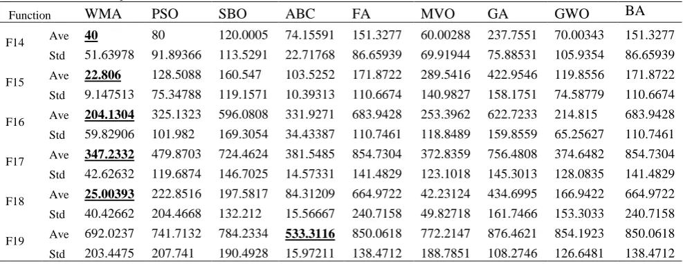
3.3. Ability to escape from local minima (functions F14–F19)
In composite functions, an optimization algorithm should strike an efficient balance between exploration and exploitation
allows local optima to be avoided. Table 9 shows the results of executing 6 composite functions in optimization algorithms.
Table 8: P-values obtained from multimodal benchmark functions
optimization algorithms in the Wilcoxon signed rank test. Accordingly, the p-value was smaller than 0.05 in all cases except
for one function (F13 in the PSO). Therefore, there was a significant difference between the WMA and other algorithms. Fig.
5 shows the convergence diagram of optimization algorithms in multimodal multimodal functions respectively . The WMA
algorithm converged than other methods because of the high exploration ability and local optimum avoidance as a result of
moving towards the global optimum.
Table 7 Results of multimodal benchmark functions
Function WMA PSO SBO ABC FA MVO GA GWO BA
F8 Ave -1.26E+04 -2.78E+03 -5.91E+03 -4.42E+03 -7.26E+03 -7.69E+03 -1.10E+04 -5.91E+03 -2.82E+03
Std 6.75E-03 4.24E+02 9.75E+02 2.52E+02 5.64E+02 8.37E+02 2.99E+02 7.76E+02 7.17E+02
F9 Ave 0.00E+00 3.88E+01 5.51E+01 2.73E+02 1.90E+02 1.17E+02 4.61E+00 2.47E+00 1.15E+02
Std 0.00E+00 1.03E+01 1.33E+01 1.18E+01 3.07E+01 3.10E+01 2.00E+00 4.14E+00 6.24E+01
F10 Ave 1.01E-15 7.94E-01 1.55E-01 1.40E+01 1.90E+01 1.85E+00 5.50E-01 1.03E-13 1.06E+01
Std 6.49E-16 1.26E+00 9.81E-02 5.72E-01 1.24E-01 4.54E-01 1.82E-01 2.25E-14 2.03E+00
F11 Ave 0.00E+00 8.33E+01 4.57E-01 5.80E+01 1.54E+02 8.59E-01 9.97E-01 4.26E-03 3.55E+01
Std 0.00E+00 7.34E+00 2.13E-01 9.43E+00 3.08E+01 6.64E-02 7.41E-02 9.99E-03 7.92E+00
F12 Ave 9.65E-05 1.45E-01 1.36E+00 2.65E+07 2.04E+06 2.33E+00 1.83E-01 4.26E-02 5.01E+03
Std 8.41E-05 1.99E-01 1.95E+00 8.60E+06 2.00E+06 1.29E+00 1.57E-01 2.20E-02 1.69E+04
F13 Ave 1.12E-03 5.80E-02 9.23E-03 6.51E+07 2.06E+07 1.81E-01 1.74E-01 6.30E-01 4.07E+05
Std 8.66E-04 2.31E-01 4.54E-03 2.26E+07 1.30E+07 9.75E-02 6.12E-02 1.92E-01 4.33E+05
Table 8 P-values obtained from multimodal benchmark functions
Function PSO SBO ABC FA MVO GA GWO BA
F8 1.92E-06 1.73E-06 1.73E-06 3.88E-06 1.13E-05 1.73E-06 1.73E-06 1.70E-06
F9 1.73E-06 1.73E-06 1.73E-06 1.73E-06 1.73E-06 1.66E-06 1.66E-06 1.73E-06
F10 1.73E-06 1.73E-06 1.73E-06 1.73E-06 1.73E-06 1.70E-06 1.70E-06 1.73E-06
F11 1.73E-06 1.73E-06 1.73E-06 1.73E-06 1.73E-06 1.70E-06 1.70E-06 1.73E-06
F12 8.73E-03 1.73E-06 1.73E-06 1.73E-06 1.73E-06 1.73E-06 1.73E-06 1.73E-06
F13 0.643517 1.73E-06 1.73E-06 1.73E-06 1.73E-06 1.73E-06 1.73E-06 1.73E-06
Fig. 5. Convergence of algorithms on multimodal benchmark functions
3.3. Ability to escape from local minima (functions F14–F19)
In composite functions, an optimization algorithm should strike an efficient balance between exploration and exploitation