ON THE SOLUTION APPROACHES OF THE BAND COLLOCATION PROBLEM
H. KUTUCU1, A. GURSOY2, M. KURT3, U. NURIYEV4,§
Abstract. This paper introduces the first genetic algorithm approach for solving the Band Collocation Problem (BCP) which is a combinatorial optimization problem that aims to reduce the hardware costs on fiber optic networks. This problem consists of finding an optimal permutation of rows of a given binary rectangular matrix representing a communication network so that the total cost of covering all 1’s by Bands is minimum. We present computational results which indicate that we can obtain almost optimal solutions of moderately large size instances (up to 96 rows and 28 columns) of the BCP within a few seconds.
Keywords: Band Collocation Problem, Dense Wavelength Division Multiplexing, Meta-heuristic Algorithms
AMS Subject Classification: 90C05, 90C09, 90B18, 93A30, 90C27, 90C59
1. Introduction
We consider a communication network in which a service provider or a source transmits data stream including m data packages to n sinks. Modern optic cable using Dense Wavelength Division Multiplexing (DWDM) technology can carry data stream coded in a givenmdifferent wavelengths [5, 17]. DWDM uses amultiplexer at the service provider to join the several signals (data) together, and ademultiplexer at the sink to split them apart. Add/Drop Multiplexers (ADM) installed at sinks facilitate flows on some wavelengths to exit the cable according to their paths.
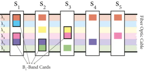
In Figure 1, a service provider transmits a data stream at different wavelengths of light simultaneously. Sink stations have special cards to control these wavelengths. Sink s1 requests the data carried on wavelengths λ1, λ2, λ4 and λ5; sink s2 requests the data carried on wavelengthsλ1,λ3,λ5 andλ6; sinks3 requests the data carried on wavelengths
1 Department of Computer Engineering, Karabuk University, Karabuk, Turkey. e-mail: [email protected]; ORCID: http://orcid.org/0000-0001-7144-7246. 2
Corresponding Author, Department of Mathematics, Ege University, Izmir, Turkey. e-mail: [email protected]; ORCID: http://orcid.org/0000-0002-0747-9806. 3
Faculty of Engineering and Natural Sciences, Bahcesehir University, Istanbul, Turkey. Izmir Bahcesehir Science and Technology High School, Izmir, Turkey.
e-mail: [email protected]; ORCID: http://orcid.org/0000-0002-7308-5661. 4 Department of Mathematics, Ege University, Izmir, Turkey.
e-mail: [email protected]; ORCID: http://orcid.org/0000-0002-3337-5859.
§ Manuscript received: December 11, 2017; accepted: March 22, 2018.
TWMS Journal of Applied and Engineering Mathematics, Vol.9, No.4 cI¸sık University, Department of Mathematics 2019; all rights reserved.
λ1,λ3,λ5 and λ6; sinks4 requests the data carried on wavelengthsλ1 and λ5 and finally sinks5 requests the data carried on wavelengths λ1 and λ4. This is described by a binary matrixA=aij: if data carried on wavelength i= 1, ..., mis requested by sink j= 1, ..., n thenaij = 1 otherwise aij = 0.
Figure 1. Cards in ADMs needed for each wavelength.
Let c0 be the cost of one card controlling only one wavelength. In this case, the total cost of the cards is 15×c0 since 15 cards are used in the above network.
In DWDM networks, there are some cards that are able to control a group of consecutive (adjacent) wavelengths as well as there are cards controlling only one single wavelength. We call this group Band. For instance, there are cards controlling two, four or eight wavelengths, that is, cards controlling Bands of length two, four or eight. The length of these Bands are generally power of two. We represent the length 2k of cards asBk-Band. Naturally,ck denotes the cost ofBk-Band.
Network hardware vendors generally price the cards so that a card cannot be more expensive than two cards in a lower level. In this regard, the following condition always holds:
2×ck> ck+1. (1)
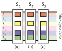
We may handle the communication from the source to five sinks in Figure 2 using cards of different lengths instead of using 15 cards of length one. If we use four cards forB1-Band and seven cards forB0-Band shown in Figure 2, then the total cost would be 4×c1+7×c0. By the condition (1), 4×c1+ 7×c0<15×c0.
Figure 2. The positions ofB0-Band andB1-Band cards.
in the ADMs. If we reorder the wavelengths as in Figure 3, then two B2-Bands and four
B1-Bands can be used to group of consecutive wavelengths. The cost of this configuration is 2×c2+ 4×c1 which is less than 4×c1+ 7×c0 by the condition (1).
Figure 3. New Bk-Bands after reordering wavelengths in Figure 1.
The Band Collocation Problem is defined formally as follows: LetA= (aij) be a binary matrix of dimensionm×nwhich represents a communication traffic wheremis the number of wavelengths and n is the number of sinks. Let 2k be the length of Bk-Band and ck be the cost of Bk-Band, where (k = 0,1, . . . ,blog2mc). Each one in a column have to be included (or covered) in (or by) exactly one band. The BCP consists of finding an optimal permutation of rows of the matrix A that minimizes the total cost of Bk-Bands in all columns.
The BCP is indeed an extended version of the Bandpass Problem (BP) introduced and formulated mathematically by Babayev et al. in 2009 [1]. The BCP was first proposed and modeled combinatorially by Nuriyev et al. in 2015 [14]. Then, Nuriyev et al. gave a mathematical formulation of the BCP as a binary integer nonlinear programming model [13]. Recent changes in ADM technology made the BP ineffective. In the BP, the length of consecutive wavelengths which are controlled by special cards are defined as a fixed number B. However, the bandpasses may be in different sizes. Furthermore, in the BP, each wavelength existing in a bandpassB corresponding to a fixedBk-Band has to carry a data for a sink. But, the technology allows an ADM to drop a wavelength even if it does not carry any information. In the BCP, a band may contain zero elements. Besides, the BP ignores costs of the programmable cards. For the state of the art techniques, the reader can refer to [14], [6] and [13].
The BP is studied by several researcher during the last decade. Li and Lin showed that the three-column BP is solvable in linear time [12].
Chen and Wang improved an approximation algorithm for the BP when B = 2 using two maximum weight matchings [2]. Their algorithm achieves a performance ratio of 220
117 ≈ 1.8805. Afterwards, Huang et al. proposed an improvement to partition a 4-matching into a number of candidate sub-4-matchings, each of which can be used to extend the first maximum weight matching. This last improved approximation algorithm in the literature has a worst-case performance ratio of 128
70−√2 ≈1.8663 [8].
The paper is organized as follows: In Section 2, we first analyze how to solve the BCP. We present a dynamic programming algorithm to find the cost of the current configuration of the wavelengths ordering. This will be used as the fitness function of genetic algorithm. In Section 3, we present some computational results for the problem and finally, give some concluding remarks in Section 4.
2. Solution Analysis of the BCP
Solving the BCP includes two stages. The first one is finding the minimum total cost to cover all 1’s in all columns using bands in the current permutation of the matrix. Covering 1’s in a column is independent from the other columns. Therefore, the numbers of B k-bands used and their coordinates would be determined for each column separately. Let us consider the second column of the matrix representing a network traffic in Figure 4.
Figure 4. A binary matrix representing the network traffic.
In what follows, there are just three of the alternatives to cover 1’s in this column:
• using four B0 item in Figure 5(a),
• using two B0 and one B1 in Figure 5(b),
• using one B0 and one B2 in Figure 5(c).
We note that a zero element can be included by any Bk-Band.
Figure 5. Some combinations of Bk-Bands used in column 2.
The costs of Bk bands used in (a), (b) and (c) are 4×c0, 2×c0 +c1 and c0 +c2 respectively. Naturally, we choose the one yielding the minimum cost.
When the number of rows and Bk-Bands increase, the number of combinations will increase exponentially. A brute-force technique is not reasonable. In [16], Nuriyeva im-prove a dynamic programming algorithm to find the coordinates ofBk-Bands and also the minimum cost to cover all 1’s of the underlying matrix. We use this algorithm given in Section 2.1 for the first stage.
2.1. The Subproblem of the BCP and Its Exact Solution. We consider each column of the traffic matrix as a sequence. The subproblem as the first stage for solving the BCP is defined as follows:
Let Q[m] be a sequence with m elements such that Q(i) ∈ {0,1}, i = 1,2, . . . , m. Let Bk-Band be a cover with 2k elements and ck be the cost of Bk-Band , where k = 0,1, ...,blog2mc.
The cost function f[Bk(Q(j), Q(j −1), . . . , Q(j −2k + 1))] to cover the elements of
Bk:Q(j), Q(j−1), ..., Q(j−2k+ 1), wherej = 1,2, ..., m, is defined as follows:
f[Bk(Q(j), . . . , Q(j−2k+1))] =
0, if the elements covered byBk are equal to 0, i.e.,
Q(j) =Q(j−1) =. . .=Q(j−2k+ 1) = 0
ck, otherwise.
The aim is to cover all nonzero elements in Q[m] with a minimum cost. Algorithm 1 finds the set of covered elements of Bk-Bands with a minimum cost. This dynamic programming algorithm runs inO(mnlog2m) time, wherem is the number of rows and n is the number of columns [16].
Algorithm 1: Dynamic Algorithm finds the minimum cost for a given traffic matrix.
Data: A binary matrixA[m, n] and costsckofBk-Bands fork= 0,1, ...,blog2mc
Result: The coordinates ofBk-Bands in each column and the total cost 1: forcolumn= 1ton do
2: forj= 1tomdo
3: Q[j] =A[j, column] 4: end for
5: R0= 0,E0=∅ 6: R1=f[B0(Q(1))] +R0 7: if Q(1) = 0then
8: E1=∅ 9: else
10: E1={1} 11: end if
12: forj= 2tom do
13: k=blog2jc
14: Rj=min{f[B0(Q(j))] +Rj−20, f[B1(Q(j), Q(j−1))] +Rj−21,
. . . , f[Bk(Q(j), Q(j−1), . . . , Q(j−2k+ 1))] +R j−2k}
15: Ej= argminelementsRj{the covered elements which gives the minimum value forRj}
16: end for
Coordinates[column]=Em 17: T otal Cost=T otal Cost+Rm 18: end for
selection methods from the union of old and new individuals until a termination criterion is satisfied.
In our GA, individuals (solutions) are represented as permutations of rows (integers) of the traffic matrix A. The general scheme of the GA is presented in pseudocode in Algorithm 2. The fitting value of an individual is the minimum band cost calculated in line 3 by Algorithm 1. Two parents are chosen using Binary Tournament Selection in line 6 at each generation. The crossover and mutation operators are applied to the individuals in lines 8 and 9, respectively, with specified probabilities. Finally, the offspring is/are inserted into the population (line 11) only if its/their fitness value is smaller than that of any parent in the current population (elitist replacement). The algorithm stops when a priori predetermined maximum number of generations is reached.
Algorithm 2:Pseudocode of the genetic algorithm for the BCP.
Data: A binary matrix A[m, n], costs ck of Bk-Bands fork= 0,1, ...,blog2mcand genetic algorithm parameters.
Result: An optimal permutation of rows of the matrix that minimizes the total cost of Bk-Bands.
1: Set iteration numbert= 1;
2: Initialize the populationP randomly;
3: Evaluate the population according to fitness value f(P);
4: Sort the population in increasing order of fitnes;
5: while termination condition is not metdo
6: t=t+ 1;
7: Select parents from the current population by binary tournament selection;
8: Crossover the selected chromosomes according tocr;
9: Mutate the selected chromosomes according tomr;
10: Evaluate new individuals;
11: Insert offspring into the population by the Elitism strategy;
12: end while
13: Return the row order having the best fitness value;
We use two crossover operators Partialy-mapped crossover (PMX) and Order crossover (OX) [4]. In examples of Figure 6 and Figure 7, all parents and offspring have 9-gene length. The examples in Figure 6 show how PMX and OX construct two offspring from two parents (chromosomes). In this figure, P i and Oi (i = 1,2) are called parents and offspring, respectively. The mutation consists in applying three different mutation methods that are Insertion, Swap and Inverse [4]. They are illustrated in Figure 7.
3. Computational Experiments
Our genetic algorithm has been implemented in C++ and tested on i7-5600U machine with a 2.60 GHz processor and 8GB RAM with a test suite composed by instances of the BCPLib [15]. 72 problem instances with known optimal solutions are chosen. We performed 10 independent runs to get reliable statistical results. We listed in Table 1 the parameters used in Algorithm 2 in all our tests. We implemented the genetic algorithm according to six combinations of two crossover and three mutation operators discussed before.
Figure 6. An example of two crossover operators.
Figure 7. An example of three mutation operators.
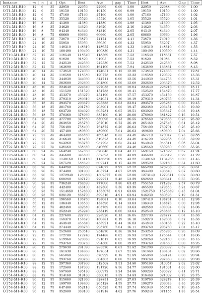
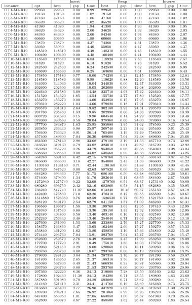
PMX crossover methods. The results of the other mutation operators (insertion and swap) can be accessed athttp://fen.ege.edu.tr/~arifgursoy/bps/BCP_Large_Tables.pdf. In Table 2, m is the number of rows, n is the number of columns, d is the density of non-zero elements of the matrix in %, Opt is the optimal value of the problem instance (matrix),Best is the best value obtained over 10 runs,Avgis the average value obtained over 10 runs, Gap is the relative error (in %) between the optimal value and the best value,T ime is the average CPU time in seconds.
The computational results which are presented in Table 3 show that the solutions ob-tained using PMX crossover are better than using OX crossover for the inverse mutation operator. We compare three mutation operators using PMX operator in Table 3. The in-verse mutation operator outperforms insertion and swap operators. The genetic algorithm with the inverse operator and PMX crossover has solved to optimality 30 instances out of 72 and CPU time varies from 1 second to 61 seconds.
Table 1. Parameters used in the GA.
Population size 200 Individuals
Selection of parents Binary Tournament Selection
Crossover PMX, OX
Mutation Insertion, Swap, Inverse
Probability of crossover (cr) 0.9 Probability of mutation (mr) 0.3
Table 2. Computational results with inverse mutation and OX, PMX
crossover methods.
OX PMX
Instance m n d Opt Best Ave gap Time Best Ave Gap Time
OT1-M1-R10 12 6 35 22950 22950 22969 0.00 1.00 22950 22988 0.00 1.00
OT1-M1-R30 12 6 35 19150 19150 19150 0.00 0.99 19150 19150 0.00 1.00
OT3-M1-R10 12 6 75 47160 47160 47160 0.00 1.00 47160 47160 0.00 1.02
OT3-M1-R30 12 6 75 35520 35520 35520 0.00 1.05 35520 35520 0.00 1.01
OT4-M1-R10 16 8 35 41380 41380 41380 0.00 1.98 41380 41390 0.00 1.95
OT4-M1-R30 16 8 35 34620 34620 34620 0.00 2.16 34620 34650 0.00 2.03
OT6-M1-R10 16 8 75 84340 84340 84340 0.00 2.05 84340 84340 0.00 2.07
OT6-M1-R30 16 8 75 60660 60660 60660 0.00 2.05 60660 60660 0.00 1.96
OT7-M1-R10 24 10 35 73870 73870 74174 0.00 4.41 73870 74019 0.00 4.36
OT7-M1-R30 24 10 35 55950 55950 56050 0.00 4.32 55950 56297 0.00 4.37
OT9-M1-R10 24 10 75 148310 148310 148652 0.00 4.33 148310 148310 0.00 4.55
OT9-M1-R30 24 10 75 100490 100490 100830 0.00 4.31 100490 100590 0.00 4.44
OT10-M1-R10 32 12 35 118540 118540 118569 0.00 7.52 118540 118651 0.00 7.57
OT10-M1-R30 32 12 35 91820 91820 91905 0.00 7.52 91820 91986 0.00 8.52
OT12-M1-R10 32 12 75 242530 242530 242530 0.00 7.53 242530 242530 0.00 8.98
OT12-M1-R30 32 12 75 163690 163690 164100 0.00 7.94 163690 163861 0.00 8.43
OT13-M1-R10 40 14 35 173850 174050 174651 0.12 12.28 173850 174665 0.00 12.81
OT13-M1-R30 40 14 35 118580 118580 120778 0.00 12.22 118580 120592 0.00 13.56
OT15-M1-R10 40 14 75 344030 344030 344711 0.00 12.56 344030 344753 0.00 13.31
OT15-M1-R30 40 14 75 202600 202600 204800 0.00 12.68 202600 203370 0.00 12.52
OT16-M1-R10 48 16 35 224640 224640 227038 0.00 18.04 224640 228216 0.00 18.11
OT16-M1-R30 48 16 35 151520 151520 154788 0.00 18.41 152520 154870 0.66 17.77
OT18-M1-R10 48 16 75 453270 453270 454190 0.00 17.57 453270 454159 0.00 16.87
OT18-M1-R30 48 16 75 279310 280310 284051 0.36 18.19 279310 280765 0.00 14.34
OT19-M1-R10 56 18 35 293570 293670 295388 0.03 23.04 293570 295283 0.00 19.45
OT19-M1-R30 56 18 35 201780 201780 203901 0.00 19.47 202380 203451 0.30 19.39
OT21-M1-R10 56 18 75 603720 604020 605281 0.05 19.51 603920 605347 0.03 19.48
OT21-M1-R30 56 18 75 378360 378960 385100 0.16 20.00 378960 381822 0.16 19.54
OT22-M1-R10 64 20 35 377700 378550 380096 0.23 26.55 378560 379333 0.23 25.39
OT22-M1-R30 64 20 35 263850 265760 267010 0.72 26.49 265460 267546 0.61 25.42
OT24-M1-R10 64 20 75 756400 758400 764872 0.26 26.63 758400 769791 0.26 25.49
OT24-M1-R30 64 20 75 457400 489600 489600 7.04 26.63 489600 489600 7.04 25.66
OT25-M1-R10 72 22 35 464300 466860 469943 0.55 34.38 467710 470047 0.73 32.88
OT25-M1-R30 72 22 35 316630 316730 319823 0.03 34.38 316720 322238 0.03 32.92
OT27-M1-R10 72 22 75 953260 953760 957295 0.05 34.43 954040 955311 0.08 33.04
OT27-M1-R30 72 22 75 538560 538560 540660 0.00 34.48 538560 539260 0.00 33.25
OT28-M1-R10 80 24 35 564240 567850 570848 0.64 43.11 569150 571622 0.87 41.24
OT28-M1-R30 80 24 35 345600 345600 357523 0.00 43.09 346600 353812 0.29 41.22
OT30-M1-R10 80 24 75 1130160 1131160 1136370 0.09 43.22 1130160 1134258 0.00 41.45
OT30-M1-R30 80 24 75 587520 588520 602741 0.17 43.28 589520 592160 0.34 41.60
OT31-M1-R10 88 26 35 644280 669560 674677 3.92 52.72 665290 678238 3.26 50.61
OT31-M1-R30 88 26 35 374400 391900 405774 4.67 52.89 384400 403840 2.67 50.60
OT33-M1-R10 88 26 75 1272940 1283860 1302577 0.86 52.88 1273140 1279511 0.02 50.80
OT33-M1-R30 88 26 75 680280 697170 722271 2.48 53.29 682680 693641 0.35 50.95
OT34-M1-R10 96 28 35 736240 764690 777006 3.86 63.42 755150 771282 2.57 60.79
OT34-M1-R30 96 28 35 442400 466100 482306 5.36 63.38 465590 479853 5.24 60.67
OT36-M1-R10 96 28 75 1514880 1528600 1535075 0.91 63.68 1521750 1525689 0.45 61.04
OT36-M1-R30 96 28 75 828120 868790 899516 4.91 63.94 846230 860593 2.19 61.31
OT37-M1-R10 56 12 35 196560 196760 198081 0.10 13.64 197410 198731 0.43 12.98
OT37-M1-R30 56 12 35 136340 136530 138596 0.14 13.63 136340 138873 0.00 12.98
OT39-M1-R10 56 12 75 402480 402680 403769 0.05 13.63 402580 403094 0.02 13.06
OT39-M1-R30 56 12 75 252240 252240 258419 0.00 13.64 252540 253836 0.12 13.10
OT40-M1-R10 64 12 35 227600 227900 228926 0.13 16.05 227700 228777 0.04 15.33
OT40-M1-R30 64 12 35 158370 158670 160881 0.19 16.10 159270 162308 0.57 15.33
OT42-M1-R10 64 12 75 453840 455840 458921 0.44 16.03 454840 460168 0.22 15.40
OT42-M1-R30 64 12 75 274440 293760 293760 7.04 16.11 293760 293760 7.04 15.47
OT43-M1-R10 72 12 35 252600 253510 254870 0.36 18.94 253250 255286 0.26 18.09
OT43-M1-R30 72 12 35 172700 172740 174488 0.02 18.93 173750 175644 0.61 18.06
OT45-M1-R10 72 12 75 519960 520060 521617 0.02 18.99 520260 522150 0.06 18.15
OT45-M1-R30 72 12 75 293760 293760 294560 0.00 19.02 293760 294560 0.00 18.25
OT46-M1-R10 80 12 35 279630 281390 283370 0.63 21.82 281290 283382 0.59 20.87
OT46-M1-R30 80 12 35 181830 184860 187654 1.67 21.88 181860 188434 0.02 20.86
OT48-M1-R10 80 12 75 565080 566080 570999 0.18 21.89 565080 569174 0.00 20.94
OT48-M1-R30 80 12 75 293760 293760 304363 0.00 21.89 293760 297850 0.00 20.98
OT49-M1-R10 88 12 35 297360 307800 312568 3.51 24.80 305160 313057 2.62 23.62
OT49-M1-R30 88 12 35 172800 187600 191720 8.56 24.77 180800 191631 4.63 23.60
OT51-M1-R10 88 12 75 587880 595180 600972 1.24 24.86 590280 593622 0.41 23.71
OT51-M1-R30 88 12 75 314160 319160 336013 1.59 24.83 316460 321002 0.73 23.75
OT52-M1-R10 96 12 35 315660 321960 328831 2.00 27.63 319760 328278 1.30 26.39
OT52-M1-R30 96 12 35 189700 198400 205128 4.59 27.73 196270 203043 3.46 26.26
OT54-M1-R10 96 12 75 647400 652110 656523 0.73 27.74 651940 653574 0.70 26.45
Table 3. Computational results for PMX crossover and three mutation operators.
Insert Swap Inverse
instance opt best gap time best gap time best gap time
OT1-M1-R10 22950 22950 0.00 0.99 22950 0.00 1.00 22950 0.00 1.00
OT1-M1-R30 19150 19150 0.00 1.02 19150 0.00 1.00 19150 0.00 1.00
OT3-M1-R10 47160 47160 0.00 1.06 47160 0.00 1.00 47160 0.00 1.02
OT3-M1-R30 35520 35520 0.00 1.02 35520 0.00 1.00 35520 0.00 1.01
OT4-M1-R10 41380 41380 0.00 1.94 41380 0.00 1.93 41380 0.00 1.95
OT4-M1-R30 34620 34620 0.00 2.00 34620 0.00 1.92 34620 0.00 2.03
OT6-M1-R10 84340 84340 0.00 2.00 84340 0.00 1.94 84340 0.00 2.07
OT6-M1-R30 60660 60660 0.00 1.99 60660 0.00 1.95 60660 0.00 1.96
OT7-M1-R10 73870 73870 0.00 4.37 74260 0.53 4.31 73870 0.00 4.36
OT7-M1-R30 55950 55950 0.00 4.40 55950 0.00 4.47 55950 0.00 4.37
OT9-M1-R10 148310 148310 0.00 4.49 148310 0.00 4.45 148310 0.00 4.55
OT9-M1-R30 100490 100490 0.00 4.48 100490 0.00 4.41 100490 0.00 4.44
OT10-M1-R10 118540 118540 0.00 6.83 118920 0.32 7.83 118540 0.00 7.57
OT10-M1-R30 91820 91820 0.00 6.13 91820 0.00 7.73 91820 0.00 8.52
OT12-M1-R10 242530 242530 0.00 6.24 242530 0.00 7.62 242530 0.00 8.98
OT12-M1-R30 163690 163690 0.00 6.25 163690 0.00 7.61 163690 0.00 8.43
4. Conclusion
In this paper, we presented a genetic algorithm by applying two crossover operators PMX, OX and three mutation operators Insertion, Inverse and Swap for solving the Band Collocation Problem. We tested all implementations of the GA using the problem instances with known optimal solutions taken from the BCPLib. We observed that the GA using PMX and inverse operators gave better results. In the literature, there is no any relevant work solving the BCP instances with known optimal solutions to compare our results. However, computational experiments show that the proposed GA is satisfactory.
As a future work, it may be interesting to test the behaviour of the GA with some local search methods such as 2-Opt, 3-Opt and λ-interchange. Our future plan is to develop other metaheuristic algorithm mentioned in Section 2.2.
Acknowledgement
The authors would like to thank the anonymous referees for their valuable comments that considerably improved the presentation of the paper. This paper is supported by the Scientific and Technological Research Council of Turkey-TUBiTAK 3001 Project (Project No:114F073).
References
[1] Babayev, D. A., Bell, G. I. and Nuriyev, U. G., (2009), The Bandpass Problem: Combinatorial Optimization and Library of Problems, Journal of Combinatorial Optimization, 18, pp. 151-172. [2] Chen, Z. Z. and Wang, L., (2012), An improved approximation algorithm for the bandpass-2
prob-lem, In Proceedings of the 6th Annual International Conference on Combinatorial Optimization and Applications (COCOA 2012), LNCS, 7402, 185-196.
[3] Dorigo, M., (1992), Optimization, Learning and Natural Algorithms, PhD thesis, Politecnico di Mi-lano.
[4] Gen M., (2006), Genetic Algorithms and Their Applications, in Springer Handbook of Engineering Statistics (eds. P. Hoang), pp. 749-773.
[5] Goralski, W. J., (1997), SONET, a Guide to Synchronous Optical Networks, McGraw-Hill, New York. [6] Gursoy, A., Tekin, A., Keserlioglu, S., Kutucu, H., Kurt M. and Nuriyev, U., (2017), An improved binary integer programming model of the Band Collocation problem, Journal of Modern Technology and Engineering, 2(1), pp. 34-42.
[7] Holland, J. H., (1975), Adaptation in Natural and Artificial Systems, University of Michigan Press. [8] Huang, L., Tong, W., Goebel, R., Liu, T. and Lin, G., (2015), A 0.5358-Approximation for Bandpass-2,
Journal of Combinatorial Optimization, 30, pp. 612-626.
[9] Kennedy, J. and Eberhart, R. C., (1985), Particle swarm optimization. In Proceedings of the IEEE International Conference on Neural Networks, 4, pp. 1942-1948.
[10] Kirkpatrick, S., Gelatt Jr, C.D. and Vecchi, M.P., (1983), Optimization by Simulated Annealing, Science, 220, pp. 671-680.
[11] Laguna, M., Sanchez-Oro, J., Marti, R. and Duarte, A., (2015), Scatter Search for the Bandpass Problem, 27th European Conference on Operational Research, July.
[12] Li, Z. and Lin, G., (2011), The Three Column Bandpass Problem is Solvable in Linear Time, Theor. Comput. Sci., 412, pp. 281-299.
[13] Nuriyev, U., Kutucu, H., Kurt, M. and Gursoy, A., (2015), The Band Collocation Problem in Telecom-munication Networks, Book of Abstracts of the 5th International Conference on Control and Opti-mization with Industrial Applications, pp. 362-365, Baku, Azerbaijan, August 27-29.
[14] Nuriyev, U., Kurt, M., Kutucu, H. and Gursoy A., (2015), The Band Collocation Problem and Its Combinatorial Model, Abstract Book of the International Conference Matematical and Computational Modelling in Science and Technology, pp. 140-142, Izmir, Turkey, August 02-07.
[15] Nuriyev U., Kurt M., Kutucu, H. and Gursoy, A., (2015), Band Collocation Problem Online Library (BCPLib): http://fen.ege.edu.tr/ arifgursoy/bps/, (2015) (LAD: December 6, 2017).
[17] Ramaswami, R., Sivarajan, K. and Sasaki, G., (1998), Optical Networks: A Practical Perspective. Morgan Kaufmann, San Francisco.
[18] Tong, W., Goebel, R., Liu, T. and Lin, G., (2014) Approximation Algorithms for the Maximum Multiple RNA Interaction Problem, Theoretical Computer Science, 556, pp. 63–70.
Hakan Kutucu received one of his master degree from International Computer Institute in 2004 and the other from the Department of Mathematics at Ege University in 2008. He completed his doctoral programme in the Department of Mathematics at Ege University in 2011. At present, he is focusing on network design problems, combinatorial optimization and mathematical modelling. He has been working in the Department of Computer Engineering at Karabuk University as an Assistant Professor since 2013.
Arif Gursoy received his master degree from the Department of Mathematics at Ege University in 2009. He also completed his doctoral programme in the same Department at Ege University in 2012. He is inteested in combinatorial optimization, mathematical modelling and soft computing. He has been working in the Department of Mathematics at Ege University as an Assistant Professor since 2013.
Mehmet Kurt received his master degree from the Department of Mathematics at Ege University in 2004. He also completed his doctoral programme in the same department at Ege University in 2010. He is inteested in combinatorial optimization, mathematical modelling, graph theory and its applications.