VOLUME 40, ARTICLE 18, PAGES 463
,
502
PUBLISHED 6 MARCH 2019
https://www.demographic-research.org/Volumes/Vol40/18/ DOI: 10.4054/DemRes.2019.40.18
Research Article
Estimating multiregional survivorship
probabilities for sparse data: An application to
immigrant populations in Australia, 1981–2011
Bernard Baffour
James Raymer
© 2019 Bernard Baffour & James Raymer.
This open-access work is published under the terms of the Creative Commons Attribution 3.0 Germany (CC BY 3.0 DE), which permits use, reproduction, and distribution in any medium, provided the original author(s) and source are given credit.
1 Introduction 464
2 Data and methodology 466
2.1 Population data 466
2.2 Mortality rates 468
2.3 Conditional survivorship proportions of interregional migration 470
2.4 Multiregional life tables 471
3 Indirect estimation of mortality and internal migration 472
3.1 Estimating age schedules of mortality 472
3.2 Log-linear smoothing of internal migration 474
3.3 Adaptation of multiregional transition probability 475
4 Illustrative example 476
4.1 Step 1: National age schedules of mortality 476
4.2 Step 2: Imposing and smoothing regional mortality schedules 477 4.3 Step 3: Log-linear modelling of origin–destination migration flow
tables
480
4.4 Step 4: Multiregional life tables 485
5 Results 485
5.1 The changing pattern of migration structures 485
5.2 Multiregional retention expectancies 489
6 Conclusion and discussion 494
7 Acknowledgements 496
Estimating multiregional survivorship probabilities for sparse data:
An application to immigrant populations in Australia, 1981–2011
Bernard Baffour1
James Raymer2
Abstract
BACKGROUND
Over 28% of the Australian population is born overseas. Understanding where immigrants have settled, and the relative attractiveness of these places in relation to others, is important for understanding the contributions of immigration to society and subnational population growth. However, subsequent demographic analyses of immigration to Australia is complicated because (1) the population is highly urbanised with over 80% living along the coast on an area roughly 3% of the country’s land mass and (2) the diversity of immigration streams results in many immigrant populations with small population numbers.
OBJECTIVE
The objective of this research is to develop methods for overcoming irregularities in sparse data on age-specific mortality and internal migration to estimate small area multiregional life tables. These life tables are useful for studying the duration of time spent, expressed in years lived, by populations living in specific geographic areas. METHODS
Multiregional life tables are calculated for different immigrant groups from 1981 to 2011 in Australia. To overcome sparse data, indirect estimation techniques are used to smooth, impose and infer age-specific probabilities of mortality and internal migration. RESULTS
We find that the country or region of birthplace is an important factor in determining both settlement and subsequent internal migration.
1 School of Demography, Australian National University, Acton, Australia. Email:[email protected].
CONCLUSIONS
Overcoming sparse data on mortality and internal migration allow for the study of the relative attractiveness of places over time for different immigrant populations in Australia. This information provides useful evidence for assessing the effectiveness of policies designed to encourage regional and rural settlement.
1. Introduction
Immigration underpins many aspects of population and societal change in Australia. According to the most recent census, over 28% of the population was born overseas (Australian Bureau of Statistics 2017). It is necessary to understand the long-term consequences of this immigration in order to determine the contributions to population change, and also to assess the Australian Government’s Department of Home Affairs (2018) policies, aimed at distributing persons to specific areas that are considered in need of immigrant labour. These include, for example, skill regional visas, pathways to permanent residence, and the regional sponsored migration scheme. They are designed to address skill shortages and encourage settlement outside state capital cities.
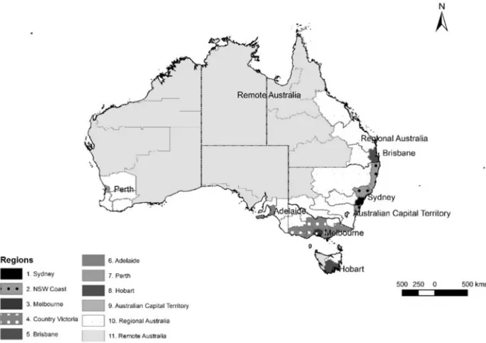
Australia is one of the least densely populated countries in the world and one of the most urbanised. This urban population is located predominantly along the south-eastern coastline from Adelaide to Brisbane. Approximately four-fifths of the population live in this narrow coastal strip of land on an area that covers roughly 3% of the country’s land mass. When considering how to subdivide the country into geographic areas this produces methodological challenges, especially when the population sizes of local authorities vary from 1,000 to 125,000 residents with an average number of around 12,000 residents (Wilson 2016).
In comparison to persons born in Australia, immigrants have been more likely to settle in major urban areas (i.e., a metropolis or a major city with at least 100,000 residents). In 2011, 64% of Australian-born people lived in a major urban area, whereas it was 85% for those born overseas. The extent to which immigrants settled in urban areas, however, differed by their country of birth. For example, 97% of the Chinese-born population and 93% of the Indian-Chinese-born population lived in urban areas but, by contrast, for the populations born in New Zealand and the United Kingdom it was 78% and 74%, respectively.
changing over time. This information is needed for understanding, for example, population redistribution, social cohesion, and the effectiveness of policies designed to attract immigrant populations to specific areas. One way to study retention is through the calculation and analysis of multiregional life tables (Rogers 1975, 1995; Willekens and Rogers 1978). The inputs required for these tables include age- and sex-specific probabilities of mortality and interregional migration. The outputs allow the study of duration expressed in expected number of life years spent in each region of the country. Although not explored in this paper, it would also be useful to compare the underlying factors that cause certain areas to exhibit high retention in relation to those that exhibit low retention.
In constructing multiregional life tables for immigrant populations in Australia, we encounter two methodological problems. First, there is sparse data, where some populations, especially in regional and remote areas, are too small to provide reliable probabilities of age-specific mortality or internal migration. This problem increases the further one goes back in time, especially for the more recently arrived immigrant populations, e.g., those born in China or India. Second, due to privacy and confidentiality concerns, the disaggregated data by age, sex, area, and country of birth have had random perturbations added to them by the Australian Bureau of Statistics (ABS) before release. Perturbation is a technique which has been developed to randomly adjust count values. When the technique is applied, all counts and totals are adjusted to prevent any identifiable information being disclosed (Chipperfield and O’Keefe 2014). These perturbations do not decrease the tabular information but the resulting adjustments can decrease the analytical utility of the data (Shlomo and Skinner 2010). The methodological approach proposed combines empirical regularities from the observed data with other auxiliary information to deal with the sparse and perturbed data.
2. Data and methodology
2.1 Population data
The population data collected for this research is derived from the quinquennial (five yearly) Australian censuses between 1981 and 2011, representing six inter-censual periods. The data contains information from 19 birthplace-specific populations comprised of 18 overseas-born population groups and the Australian-born. The birthplace categories of the overseas-born population represent a mixture of countries and world regions. In 2011 the total size of the overseas-born population was 5.8 million persons and of the Australian-born population 16.5 million persons. Each of the 18 immigrant birthplaces accounts for a relatively large proportion of the total overseas-born population in Australia, ranging from 1% for the Indonesian-overseas-born population to 21% for the United Kingdom-born population. For illustration and space reasons, this research focuses on the four largest immigrant populations, born in the United Kingdom, New Zealand, China, and India, which comprise 21%, 9%, 6%, and 6% of the overseas-born population, respectively.
The birthplace-specific data was commissioned from the Australian Bureau of Statistics, which provided information based on the Statistical Division geography from Australian Standard Geographical Classification. The geographic boundaries of this data are not consistent over time (Australian Bureau of Statistics 2011). For any given year, there are around 60 Statistical Divisions. For example, there were 58 Statistical Divisions in 1981 and 62 in 2011. To produce a consistent geography over time, we used simple rules that either assumed the boundary changes were insubstantial (i.e., if the boundary change resulted in only a small amount of population change) or merged multiple geographic areas into single (larger) ones (see Guan (2018) for details on the construction of the 47 harmonised geographic areas). These rules produced a meaningful geography for studying subsequent migration of immigrant populations across 47 areas and over six time periods. The only geographic area that required additional input was Darwin in the Northern Territory. Here, the population size was altered to correspond to the geographic area change.
the 47 geographical areas. Even at this geographic level, there are considerable sparse data issues that have to be addressed.
Figure 1: Map of the eleven geographic areas for Australia
15% in remote areas, and 49% in very remote areas (Australian Bureau of Statistics 2013).
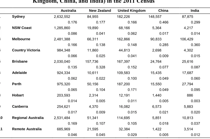
Table 1: Regional population counts (with column proportions) in Australia for selected countries of birth (Australia, New Zealand, United Kingdom, China, and India) in the 2011 Census
Australia New Zealand United Kingdom China India 1 Sydney 2,632,552 84,955 182,226 148,557 87,875
0.176 0.177 0.166 0.466 0.299
2 NSW Coast 1,285,860 19,890 68,166 5,364 4,217
0.086 0.041 0.062 0.017 0.014
3 Melbourne 2,481,388 66,311 162,866 90,833 106,429
0.166 0.138 0.148 0.285 0.360
4 Country Victoria 984,348 11,860 44,813 2,698 4,302
0.066 0.025 0.041 0.009 0.015
5 Brisbane 2,030,040 157,736 167,397 24,764 25,616
0.135 0.328 0.152 0.077 0.087
6 Adelaide 924,334 10,611 109,583 15,435 17,687
0.062 0.022 0.100 0.049 0.060
7 Perth 975,320 50,156 187,200 15,550 27,794
0.065 0.104 0.171 0.049 0.095
8 Hobart 203,593 2,314 12,191 1,440 886
0.014 0.005 0.011 0.005 0.003
9 Canberra 254,621 4,370 16,082 6,573 5,883
0.017 0.009 0.015 0.021 0.020
10 Regional Australia 2,531,484 51,341 114,695 5,851 10,813
0.169 0.107 0.105 0.018 0.037
11 Remote Australia 685,969 21,595 32,384 1,422 3,514
0.046 0.045 0.029 0.005 0.012
2.2 Mortality rates
Consider the age-specific mortality rates for persons living in Australia and born in the United Kingdom, China, India, and Australia presented in Figure 2 for the two periods 1981–1986 and 2006–2011. The lines in the figures generally reflect the typical mortality curve for a developed country, i.e., a rapidly decreasing rate of mortality in the early years of life, followed by a sharp increase in mortality during the teenage years, then a plateau for young adults, subsequently followed by a steady increase from around 30 years of age. While this pattern is apparent for the Australian-born population, the observed mortality rates of the immigrant groups are subject to more fluctuations and, in some instances, zero values, e.g., Chinese-born population during the 1981–1986 period at very young ages. The reason why this population may have zero deaths is likely due to its young population age structure with few children present, or missing death counts.
Figure 2: Male age-specific mortality rates (logged) for the populations born in Australia, United Kingdom, New Zealand, China, and India: 1981– 1986 and 2006–2011
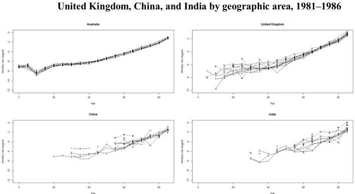
Figure 3: Age-specific mortality rates (logged) for males born in Australia, the United Kingdom, China, and India by geographic area, 1981–1986
Note: □ Sydney, o Melbourne, ∆ Brisbane, + Adelaide, x Perth, ◊ Australian Capital Territory,∇ New South Wales Coast,∎ Country Victoria, * Greater Hobart, % Regional Australia, # Remote Australia.
2.3 Conditional survivorship proportions of interregional migration
The conditional survivorship proportion of migration represents the number of persons in a particular age group who migrated out of a region during a time interval, divided by the total number of persons in that age group who lived in the region at the beginning of the time interval. As data on ‘where were you living five years ago?’ is collected at the end of the time interval, the persons must have survived in order to be counted in the census. Conditional survivorship proportions provide the inputs to calculate multiregional life tables under the ‘Option 2’ method in Rogers (1995).
produce irregular conditional survivorship proportions when disaggregated by origin, destination, sex, and age group.
2.4 Multiregional life tables
Multiregional demography (Rogers 1975, 1995; Willekens and Rogers 1978) offers unique insights into components of change by considering subpopulations that are interconnected by origin–destination migration flows. A particularly useful way of understanding demographic change of subpopulations is to examine them through a multiregional life table. A useful statistic provided by a multiregional life table is the average expectation of life beyond age in each region. This is calculated by applying age-specific probabilities of survival to hypothetical cohorts of babies, and then observing at each age and current region of residence their average expected length of remaining life years to be spent in each of the regions in the population system (Rogers 1973; Willekens and Rogers 1978).
In Table 2 we present the multiregional life expectancies for Australian-born males at age zero based on the 2006–2011 period data for age-specific mortality and conditional survivorship proportions of interregional migration. Here we see substantial differences in life expectancy depending on the area where they were residing at age zero. For instance, a baby boy born in Sydney is expected to live to an average age of 78.1 years, of which around 60% will be spent residing in the same region. However, if he were to be born in Canberra his expected life expectancy would increase to 78.3 years, but only around 40% of his years would be spent residing in the same area. For Remote Australia, life expectancy drops to 76.4 years with only 30% of years being spent in the same (large) area.
Table 2: Multi-regional life tables: expectations of life at birth, by region of residence: Males born in Australia (2006–2011)
Destination S y d n e y N S W C o a s t M e lb o u rn e C o u n tr y V ic to ri a B ri s b a n e A d e la id e P e rt h G re a te r H o b a rt C a n b e rr a R e g io n a l A u s tr a li a R e m o te A u s tr a li a T o ta ls U n ir e g io n a l Origin
Sydney 49.2 7.3 3.2 1.2 5.6 1.1 1.5 0.4 1.1 6.5 1.3 78.1 78.4
NSW Coast 9.5 38.6 3.2 1.5 8.8 1.2 1.7 0.4 1.2 9.6 2.0 77.7 77.5
Melbourne 2.3 1.4 53.4 8.6 3.5 1.2 1.5 0.4 0.6 4.5 1.2 78.5 79.0
Country Vic. 1.9 1.9 16.6 39.6 4.3 1.5 1.9 0.4 0.6 7.4 1.9 77.8 77.6
Brisbane 3.7 4.0 4.0 1.9 45.2 1.5 1.9 0.6 0.8 11.5 2.7 77.8 78.3
Adelaide 2.4 1.8 3.9 1.7 4.4 49.7 2.0 0.5 0.8 8.1 3.2 78.1 78.6
Perth 2.6 2.0 4.4 1.8 4.2 1.7 43.6 0.5 0.7 11.2 5.1 77.8 78.3
Hobart 3.1 2.3 6.4 2.4 5.8 1.6 2.4 41.8 1.0 7.7 2.9 77.3 76.8
Canberra 7.0 5.0 6.1 2.2 8.5 2.3 2.4 0.5 28.9 13.4 1.9 78.3 79.8
Regional Aus. 4.6 4.9 4.8 3.1 9.8 3.2 4.4 0.7 1.5 36.6 3.8 77.4 76.9
Remote Aus. 2.8 3.2 3.8 2.4 8.1 4.8 7.5 1.1 0.8 15.6 26.3 76.4 73.9
3. Indirect estimation of mortality and internal migration
3.1 Estimating age schedules of mortality
Recognising that age schedules of mortality, fertility, and migration follow remarkably persistent patterns over time and across space, demographers have summarized and codified these regularities through parameterised model schedules (Booth and Tickle 2008; Rogers and Raymer 1999). The most developed are models of age-specific mortality, which can be represented by a variety of functions, such as the Gompertz or Makeham mathematical models, Brass’ (1971) relational model, or Heligman and Pollard’s (1980) parameterized model. Lee and Carter (1992) developed a widely used forecasting method that makes use of the regularity typically found in age patterns and trends over time, but it makes strong assumptions about the functional form of mortality and is dependent on the availability of good historical time series data.
on historical and theoretical considerations. However, these models require long historical time series data to overcome the various model constraints and data inadequacies (Hyndman, Booth, and Yasmeen 2013).
Bayesian models have also been developed which estimate the small-area mortality rates and life expectancies through borrowing strength across ages, sexes, times, and locations (Alexander, Zagheni, and Barbieri 2017). However, these models can be complex and contain high levels of dimensionality and large numbers of parameters to be estimated (Congdon 2009, 2014). Furthermore, in cases where the data is of poor quality, relational methods rely on having an accurate ‘standard’ mortality schedule for benchmarking and producing accurate estimates. In our application, where the interest is in the differences between both small areas and immigrant groups, the choice of a standard schedule is not clear. Furthermore, the birthplace-age-area specific mortality rates can be subject to instability and, as such, relational model parameters may not accurately describe and capture the age pattern of mortality experienced by the immigrant populations in the local areas (De Beer 2012).
Statistical parametric and non-parametric models may be used for estimating demographic components using regression and time series methods (see, e.g., Bijak and Wiśniowski 2010; Gerland et al. 2014; Hyndman and Ullah 2007; Hyndman, Booth, and Yasmeen 2013; Raftery et al. 2012; Renshaw 1991; Haberman and Renshaw 1996). However, these approaches often require higher-order polynomial and complex interaction terms, which may lead to issues around model fitting. Here, splines may be employed to improve the model fit through smoothing (Currie, Durban, and Eilers 2004; Dodd et al. 2018); for example, by using P-splines (Currie and Durban 2002; Eilers and Marx 1996). The optimal smoothing parameters are chosen subject to a trade-off between model fit and model complexity, i.e., through using the Akaike Information Criterion, AIC (Akaike 1973). Spline-based methods help the mortality functions to be ‘well-behaved’ while relying on the generalised linear modelling framework (Currie, Durban, and Eilers 2006a; Dodd et al. 2018). In addition, since mortality displays regular patterns, these smoothing approaches are considered more natural for representing mortality changes than imposing a fairly rigid model structure (Carmada 2012; Currie, Durban, and Eilers 2004, 2006a, 2006b).
permanent residence visa status and some temporary visa statuses. This policy is designed to (1) ensure that immigrants are free from any diseases considered to be a threat to Australian society, and (2) prevent significant healthcare costs to Australian taxpayers. Thus, the overseas-born population is expected to have commonalities across their age-specific mortality patterns. Moreover, this approach provides estimates of the age schedules of mortality with sufficient variation to discern differences in total immigrant mortality over time and across space.
Our approach is specified as follows. First, consider the counts of deaths by age group. For a given population in age group in region , the total number of deaths Di(x) follows a Poisson distribution: Di(x)~Poisson[Ei(x)*μi(x)], where the hazard (or force of mortality) is μi(x) and the exposure (at-risk) population is 5/2[Ei1(x)+ Ei2(x)].
Ei1(x) andEi2(x) denote the population sizes at the beginning and end of the five-year
interval, respectively. The age-specific death rates are thusmi(x) =Di(x) / {5/2[Ei1(x)+
Ei2(x)]}. In instances when the age-specific death rates,mi(x), cannot be computed (due
to either no deaths or no populations, or both, we initially replace themi(x) with the corresponding national rates for the specified immigrant population, and the total overseas-born rates for cases when the national age-specific rates are unavailable. Second, the computation of the spline smoothing was undertaken in R using the MortalitySmooth package (Carmada 2012). The smoothing of the Poisson death rates was undertaken using the ‘Mort1DSmooth’ function. While the Poisson distribution provides a suitable model for analysing count data, the requirement that the mean and variance should be equal is generally restrictive and impractical. This is because demographic data is often over-dispersed and displays extra variation. As such, we specify the option ‘overdispersion=TRUE’, which allows the spline-based smoothing to accommodate overdispersion. After computing the mortality rates, they are transformed into age-specific mortality probabilities, ( ), for use in the multiregional life table calculations.
3.2 Log-linear smoothing of internal migration
Log-linear models are useful for describing and discerning patterns that underlie spatial data presented in the form of contingency tables. Through considering the regularities in the age, spatial, and temporal patterns of the migration flows, smoothed estimates of interregional migration can be obtained by fitting unsaturated log-linear models (Raymer and Rogers 2007; Rogers, Raymer, and Little 2010).
and sex, respectively. We specify the full (saturated) log-linear model for analysing migration flow tables over space as:
log = + + + + + ( , , , )
+ ( , , , ) + ℎ( , , , ) + ( , , , )
where ( , , , ), ( , , , ),ℎ( , , , ), ( , , , )represent sets of two-way interactions, three-way interactions, and the four-way interaction between origin, destination, age, and sex, respectively. This model can be contrasted with various unsaturated models which assume, for example, that the internal migration flows are distributed according to the marginal totals across origin, age, and sex, specified as:
log = + + + + .
The appropriateness of the reduced model is determined by fitting the predicted flows to the observed flows and by using the likelihood ratio statistic or Chi-square statistic to evaluate the goodness of fit. If the reduced form fits the observed data well, then the model may be considered appropriate for estimating the flows.
3.3 Adaptation of multiregional transition probability
Key to the multiregional life table estimation is the conditional survivorship proportion of interregional migration, denoted as pij(x), which is the probability that a person in regioni at exact agexwill reside in regionj at exact agex+5, with pii(x) denoting the probability of staying. The life table functions of the hypothetical population are computed by combining age-specific probabilities of dying and out-migrating to the different component regions in the multiregional population system.
We first obtain the appropriate set of mortality probabilities,qi(x), which give the probability of dying at each age for each of the eleven regions. We can then derive the matrix of probabilities of out-migration as:
P(x)=
p11(x) ⋯ p1K(x)
⋮ ⋱ ⋮
pK1(x) ⋯ pKK(x) , i= 1, …,K;j= 1, ...,K.
out-migration probability can be computed as pij(x) = Nij(x) / Ni+(x), where Nij(x) is the number of people who start off in region i at agex and move to region j at x+5, and Ni+(x) is the total number of people agedx in region i. Following Rogers (1975), we make the assumption that an individual makes one move during that time period. Similarly,pii(x) =Nii(x) /Ni+(x)= 1 –∑ ( ) − ( ), whereNii(x) is the number of non-movers or persons remaining and ( ) is the probability of an individual in region i dying between ages x and x +5. However, due to inaccuracies in the at-risk age-specific populations and statistical perturbations for disclosure control, there are a number of inconsistencies in the computations. We therefore apply an adjustment and re-scaling procedure, wherepij(x) =Nij(x) / ∑i,jNij(x) (adjustment) andp*ij(x) = [pij(x) / ∑i,jpij(x)][1–qi(x)] (rescaling). The adjustment corrects for the inconsistent populations at risk, while the rescaling ensures that regional age-specific differences in mortality are taken into account, and always sum to one.
4. Illustrative example
In this section we demonstrate the various steps to repair and smooth the sparse regional mortality and migration data. For illustration, the methodology is implemented for the Australian-born population and the immigrant populations born in the United Kingdom, New Zealand, China, and India. To show how these populations have changed over time, we focus on two periods: 1981–1986 and 2006–2011. The age patterns of Chinese-born mortality and interregional migration exhibit irregularities and, in some instances, observed zeros. Both situations complicate the construction of realistic probabilities. At the regional level there are even more instances of ‘jagged’ mortality schedules and zero values, especially at younger ages (e.g., there are no reported deaths for persons under 25 years of age for some regions in Australia). Regional mortality rates for the Australian-born population, on the other hand, have much larger numbers and exhibit the expected age patterns of mortality. Immigrants born in the United Kingdom exhibit mortality patterns similar to the Australian-born, due to their longer history of migration to Australia and larger population size. However, for smaller capital city regions and regional and remote areas there are some irregularities present in the age profiles as a result of their relatively small population sizes.
4.1 Step 1: National age schedules of mortality
The total overseas-born age schedules are used as a basis for overcoming zero values and irregular patterns in the birthplace-specific immigrant mortality data, with males and females treated separately. That is, when ‘zero’ mortality counts are present in the data, the age-specific mortality rates of the total overseas-born population are imposed. One thing to note is that the mortality schedules of the total overseas-born population exhibit somewhat irregular patterns in comparison to the Australian-born population. This occurrence is due to the smaller counts in the data and the concentration of young and healthy adults in the immigration flows (Kennedy et al. 2014; Newbold and Danforth 2003; Singh and Siahpush 2002).
Figure 4: Observed age-specific male mortality rates (logged) for the Australian-born and overseas-born populations: 1981–1986 and 2006–2011
4.2 Step 2: Imposing and smoothing regional mortality schedules
deaths, or having no reported resident populations. There are also some instances where every person in a certain age group dies. These are all undesirable features due to the sparse data. To overcome these issues, we replace any zero values with the total overseas-born male or female mortality rates and then smooth the data using splines. Figure 5: Age-specific mortality rates (logged) for male populations born in
Australia, China, and the United Kingdom and located in Sydney, Adelaide, and Remote Australia: 1981–1986 and 2006–2011
Figure 5: (Continued)
b) United Kingdom
Note: o = reported; + = after smoothing.
lack of reliable information on the age-specific mortality patterns across areas for the different immigrant populations. Similar patterns are observed for the period 2006– 2011, except that the reported age patterns are closer to the smoothed patterns, which can be attributed to higher levels of migration.
4.3 Step 3: Log-linear modelling of origin–destination migration flow tables
In the third step we address irregular patterns in the interregional migration data by categorising it into three groups, based on data availability: (a) good quality data (b) irregular data with discernible patterns, and (c) poor quality data with no discernible patterns. For group (a) no smoothing is required and the observed data is analysed as is. For (b), unsaturated log-linear models are used to smooth the age-specific flow data. For (c) the age and migration patterns from other populations are imposed.
Understanding that there are two different processes influencing the distribution of stayers and movers, we fit different log-linear models for movers and stayers (i.e., those that remain in their area of residence during the five-year time period). This is standard practice in the analysis of migration tables, where the stayers are represented as the diagonal elements (Agresti 2002: 423–428). The final ‘best fitting’ model was based on investigating which model captures the spatial structure of migration, while maximizing the model fit through reducing the number of model parameters. As such, the final model chosen for movers contained two-way interactions between origin and destination and between age and sex. The final model for stayers was similar but had two-way interactions between age and sex and between origin and sex. We investigated adding more interactions for both the stayer and migrant models, but these were found to be problematic because of the large number of zeros.
Since the United Kingdom-born immigrant population is considerably larger than the other immigrant populations, we were able to fit a more complex model. For movers, this model contained additional two-way interactions between origin and age, destination and age, origin and sex, and destination and sex, whereas for stayers there was an additional origin and age interaction. The quality of the Australian-born migration data was considered good and, as such, there was no need to smooth the internal migration flows.
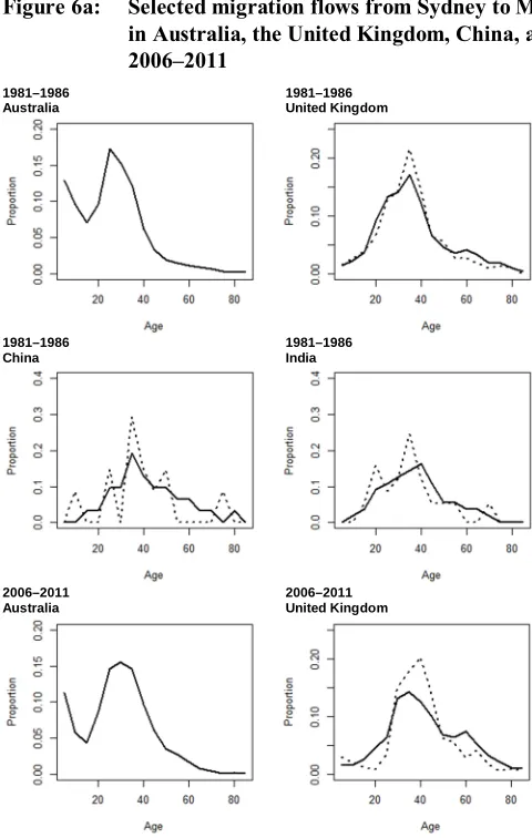
Kingdom, China, and India. In each plot the age profile of migration is presented before and after log-linear smoothing, except for the Australian-born population where no smoothing was applied. These plots provide an indication of the effect of randomness on the age and spatial patterns of migration due to variation in the size of the immigrant populations, which is especially noticeable in the smaller flows.
Figure 6a: Selected migration flows from Sydney to Melbourne for persons born in Australia, the United Kingdom, China, and India: 1981–1986 and 2006–2011
1981–1986 1981–1986
Australia United Kingdom
1981–1986 1981–1986
China India
2006–2011 2006–2011
Figure 6a: (Continued)
2006–2011 2006–2011
China India
Note: Dashed line = reported; Solid line = after log-linear smoothing.
Figure 6b: Selected migration flows from Sydney to Adelaide for persons born in Australia, the United Kingdom, China, and India: 1981–1986 and 2006–2011
1981–1986 1981–1986
Australia United Kingdom
1981–1986 1981–1986
Figure 6b: (Continued)
2006–2011 2006–2011
Australia United Kingdom
2006–2011 2006–2011
China India
Note: Dashed line = reported; Solid line = after log-linear smoothing.
Figure 6c: Selected migration flows from Sydney to Remote Australia for persons born in Australia, the United Kingdom, China, and India: 1981–1986 and 2006–2011
1981–1986 1981–1986
Figure 6c: (Continued)
1981–1986 1981–1986
China India
2006–2011 2006–2011
Australia United Kingdom
2006–2011 2006–2011
China India
Note: Dashed line = reported; Solid line = after log-linear smoothing.
3.2). Figure 6c presents the age profiles of ‘small’ flows from Sydney to Remote Australia, for the four sub-populations: Australian-born, United Kingdom-born, China-born and India-China-born. All reported flows for both periods, except for the Australian-China-born population, contain irregularities, likely due to the small cell size of the flows. Here, the smoothing appears to work well, whilst also capturing the different shapes of interregional migration.
4.4 Step 4: Multiregional life tables
The final stage involved calculating both the uniregional and multiregional life tables for each of the Australian-born and overseas-born populations. We focus on the multiregional life expectancies at age 25 years to capture the peak ages of recent immigrants. Regional retention is determined by analysing the diagonals of the multiregional life tables (i.e., stayers). Regional attractiveness is determined by analysing the off-diagonal elements of the multiregional life table. The full set of multiregional life tables calculated for all 19 birthplace groups by sex and all six time periods are presented in thesupplementary material.
5. Results
The previous sections have set out the methodological approach for understanding the dynamics of interregional migration in Australia, by place of birth, over the period 1981 to 2011. We now illustrate the resulting multiregional life tables, accounting for sparsity and inadequate mortality and migration data, for two time periods (1981–1986 and 2006–2011) and the top-five largest countries of birth (Australia, New Zealand, United Kingdom, China, and India).
5.1 The changing pattern of migration structures
eleven states, and the survivorship curves reflect the time spent in each of these regions, depending on the region of origin (i.e., Sydney, Melbourne, Adelaide, and Remote Australia). The white area under each survivorship curve captures the proportion of the cohort that remains in the same region (i.e., non-movers).
The results in Figure 7 show that the Australian-born and Chinese-born populations experience very different survivorships. For the Australian-born population that live in Sydney, Melbourne, and Adelaide, there is considerable retention across age groups in contrast to those that live in Remote Australia. These patterns are different for the Chinese-born population. For this population, the survivorship curves for those who live in Sydney and Melbourne exhibit a less steep decline in mortality with time and provide evidence of higher retention in those cities when compared with those in Adelaide and Remote Australia. Also, reflecting the fact that children are unlikely to immigrate to Remote Australia, the multiregional survivorship curve is one at the early ages. Further, Sydney and Melbourne are especially attractive as destinations for the Chinese-born internal migrants.
Figure 7: Male multiregional survivorship proportions for selected regions in Australia, 2006–2011: Australian-born and China-born persons
Figure 7: (Continued)
China: Sydney
Australia: Melbourne
Figure 7: (Continued)
Australia: Adelaide
Figure 7: (Continued)
Australia: Remote Australia
China: Remote Australia
5.2 Multiregional retention expectancies
We now provide an indication of how attractive different regions are to immigrant populations. For this we focus on the number of remaining years of life that an individual can be expected to live in given region, at a particular age, provided that they remain in Australia. For ease of comparison and interpretation, we convert these multiregional life expectancies into percentages of remaining life.
Australian-born population, compared to males born in the United Kingdom, New Zealand, China, and India. Similar patterns were found for females. We are also interested in ascertaining whether there are regional differences, and for this purpose we look at Sydney, Melbourne, Adelaide, and Remote Australia, to represent a broad spectrum of regional variability. The retention rates, highlighted in the figures, are the expected percentages of remaining life that will be spent in the particular (reference) region, assuming that they do not emigrate out of Australia. These retention rates provide a useful measure of regional attractiveness and facilitate comparison across the different groups.
The results show that different immigrant groups have varying attractiveness for different regions. Males born in China and India are clearly attracted to Sydney and Melbourne, and this has increased over time. Even when they start off living in other locations, they display strong likelihoods of moving to these two cities. However, this strong preference for Sydney and Melbourne is not true for male immigrants born in the United Kingdom or New Zealand, or for those born in Australia. For Remote Australia the retention rates are much lower, and in particular there is a very low likelihood of immigrants from India arriving in remote Australia and staying there. Males born in Australia are roughly seven times more likely to remain in remote Australia than Indian-born migrants.
Figure 8a: Multiregional life expectancies (percentages) for males aged 25 years old born in Australia, United Kingdom, New Zealand, China, and India, 1981–1986 and 2006–2011: Sydney and Melbourne
Figure 8a: (Continued)
2006–2011 Sydney
Figure 8a: (Continued)
2006–2011 Melbourne
Note: The corresponding multiregional life expectancy for each country of birth is provided in parenthesis.
Figure 8b: Multiregional life expectancies (percentages) for males aged 25 years old born in Australia, United Kingdom, New Zealand, China, and India, 1981–1986 and 2006–2011: Adelaide and Remote Australia
Figure 8b: (Continued)
2006–2011 Adelaide
Figure 8b: (Continued)
2006–2011 Remote Australia
Note: The corresponding multiregional life expectancy for each country of birth is provided in parenthesis.
6. Conclusion and discussion
In Australia, immigration is a major political and developmental issue, and there are specific policies designed to encourage immigrants to settle in regional and more remote areas for population growth and economic development (Hugo 2008). The aim of these policies is to address skill shortages, attract overseas businesses, and spread the population more evenly across the country (Department of Home Affairs 2018). To understand their effectiveness we need information that moves beyond the analysis of just immigration flows towards measures that capture the durations of time expected to be spent in particular places. Combining mortality data and internal migration data of immigrant populations in a multiregional life table provides the analyst with such measures.
and their uneven population distribution. Moreover, many of the recent immigrant groups are too small in population size and young in age composition to have experienced mortality. This creates a problem when trying to understand the probability of dying and calculation of life tables in relation to other immigrant groups.
We developed smoothing methods for age-specific mortality rates that combined observed death rates for particular immigrant groups with data from all overseas immigrants. We also used log-linear models to improve the sparse interregional migration flow data. By fitting unsaturated models to them, we were able to borrow strength from marginal distributions contained in the data, and use these to calculate more plausible conditional survivorship proportions of interregional migration. We envision the framework and methodology presented in this paper being useful and extendable to other contexts that involve the study of demographic change among any set of small subpopulations that include other types of age-specific transitions, such as between education levels, health statuses, and employment statuses.
One aspect we did not include in our methodology is the inclusion of uncertainty in the estimates. While a considerable amount of research is available on integrating uncertainty in age-specific mortality estimates, integrating uncertainty in a multiregional context is considerably more difficult. This is especially true in the presence of poor or sparse data (see Gill 1992: 273). To include uncertainty in the model framework, one would have to account for the sparseness, build in the complex correlation structures (region, age, sex, time), and account for the differing levels of uncertainty between the different types of data on internal migration and mortality. Wiśniowski and Raymer (2016) have developed a prototype Bayesian multiregional population-forecasting model for regions in England that could provide a basis for such work.
Lastly, we demonstrated the usefulness of multiregional life tables for analysing the demographic consequences of immigration and found striking differences between the populations born in Australia, the United Kingdom, China, and India. Without addressing the sparse nature of the data, these measures would be unattainable and our understanding of the long-term consequences of migration would be limited. Future research will focus on exploring these results in more detail and over time, as well as for other immigrant groups.
subnational populations as a system, as opposed to a set of ‘independent’ regions, greatly enhances the study of demographic change and interaction.
In conclusion, this research provides a methodological framework for overcoming issues associated with using sparse data to conduct detailed demographic analyses. We focused on improving immigrant mortality and international migration data and the calculation of multiregional life tables. We hope this research will inspire similar research in other high-immigration countries. We believe that as diverse streams of migration continue, migration will become increasingly important for understanding demographic change.
7. Acknowledgements
References
Agresti, A. (2002). Categorical data analysis. New York: Wiley. doi:10.1002/0471 249688.
Akaike, H. (1973). Information theory and an extension of the maximum likelihood principle. In: Petrov, B. and Czaki, F. (eds.).Second international symposium on information theory. Budapest: Akademiai Kiado: 267–281.
Alexander, M., Zagheni, E., and Barbieri, M. (2017). A flexible Bayesian model for estimating subnational mortality. Demography 54(6): 2025–2041. doi:10.1007/
s13524-017-0618-7.
Australian Bureau of Statistics (2011). Australian Standard Geographical Classification (ASGC): Catalogue No. 1216.0 [electronic resource]. Canberra: Australian Bureau of Statistics.http://www.abs.gov.au/ausstats/[email protected]/mf/1216.0. Australian Bureau of Statistics (2013). Estimates of Aboriginal and Torres Strait
Islander Australians, June 2011: Catalogue No. 3238.0.55.001 [electronic resource]. Canberra: Australian Bureau of Statistics. http://www.abs.gov.au/
ausstats/[email protected]/lookup/3238.0.55.001Media%20Release1June%202011.
Australian Bureau of Statistics (2017). Migration, Australia, 2015–16: Catalogue No. 3412.0 [electronic resource]. Canberra: Australian Bureau of Statistics.
http://www.abs.gov.au/ausstats/[email protected]/lookup/3412.0Media%20Release1201 5-16.
Bijak, J. andWiśniowski, A. (2010). Bayesian forecasting of immigration to selected European countries by using expert knowledge. Journal of the Royal Statistical Society, Series A (Statistics in Society) 173(4): 775–796.
doi:10.1111/j.1467-985X.2009.00635.x.
Booth, H. and Tickle, L. (2008). Mortality modelling and forecasting: A review of methods. Annals of Actuarial Science 3(1–2): 3–43. doi:10.1017/S1748499
500000440.
Brass, W. (1971). On the scale of mortality. In: Brass, W. (ed.).Biological aspects of demography. London: Taylor and Francis: 69–110.
Chipperfield, J.O. and O’Keefe, C.M. (2014). Disclosure-protected inference using generalised linear models. International Statistical Review 82(3): 371–391.
doi:10.1111/insr.12054.
Congdon, P. (2009). Life expectancies for small areas: A Bayesian random effects methodology. International Statistical Review 77(2): 222–240. doi:10.1111/j.
1751-5823.2009.00080.x.
Congdon, P. (2014). Estimating life expectancies for US small areas: A regression framework. Journal of Geographical Systems 16: 1–18. doi:10.1007/s10109-013-0177-4.
Currie, I.D. and Durban, M. (2002). Flexible smoothing with P-splines: A unified approach. Statistical Modelling 2(4): 333–349. doi:10.1191/1471082x02st 039ob.
Currie, I.D., Durban, M., and Eilers, P.H.C. (2004). Smoothing and forecasting mortality rates. Statistical Modelling 4(4): 279–298. doi:10.1191/1471082X 04st080oa.
Currie, I.D., Durban, M., and Eilers, P.H.C. (2006a). Generalized linear array models with applications to multidimensional smoothing. Journal of the Royal Statistical Society B (Statistical Methodology) 68(2): 259–280. doi:10.1111/j.
1467-9868.2006.00543.x.
Currie, I.D., Durban, M., and Eilers, P.H.C. (2006b). Smoothing and forecasting mortality rates. Statistical Modelling 4(4): 279–298. doi:10.1191/1471082X 04st080oa.
De Beer, J. (2011). A new relational method for smoothing and projecting age-specific fertility rates: TOPALS. Demographic Research 24(18): 409–454.
doi:10.4054/DemRes.2011.24.18.
De Beer, J. (2012). Smoothing and projecting age-specific probabilities of death by TOPALS. Demographic Research 27(20): 543–592. doi:10.4054/DemRes. 2012.27.20.
Department of Home Affairs (2018). Fact sheet: State specific regional migration [electronic resource]. Canberra: Department of Home Affairs.
Dodd, E., Forster, J.J., Bijak, J., and Smith, P.W.F. (2018). Smoothing mortality data: The English life table, 2010–2012.Journal of Royal Statistical Society,Series A (Statistics in Society) 181(3): 717–735.doi:10.1111/rssa.12309.
Eilers, P.H.C. and Marx, B.D. (1996). Flexible smoothing with B-splines and penalties.Statistical Science 11(2): 89–121.doi:10.1214/ss/1038425655. Gerland, P., Raftery, A.E., Ševčíková, H., Li, N., Gu, D., Spoorenberg, T., Alkema, L.,
Fosdick, B.K., Chunn, J.L., Lalic, N., Bay, G., Buettner, T., Heilig, G.K., and Wilmoth, J. (2014). World population stabilization unlikely this century.Science 346(6206): 234–237.doi:10.1126/science.1257469.
Gill, R.D. (1992). Multistate life-tables and regression models. Mathematical Population Studies 3(4): 259–276.doi:10.1080/08898489209525345.
Guan, Q. (2018). Creating population-based consistent geography over 1981–2011 [unpublished manuscript]. Canberra: School of Demography, Australian National University. http://demography.cass.anu.edu.au/sites/default/files/docs/ 2018/11/Document_on_Creating_Population-based_Consistent_Geography_
over_1981-2011.pdf.
Haberman, S. and Renshaw, A. (1996). Generalized linear models and actuarial science. Journal of the Royal Statistical Society: Series D (The Statistician)
45(4): 407–436.doi:10.2307/2988543.
Heligman, L. and Pollard, J.H. (1980). The age pattern of mortality. Journal of the Institute of Actuaries 107(1): 49–80.doi:10.1017/S0020268100040257. Hugo, G. (2008). Australia’s state-specific and regional migration scheme: An
assessment of its impacts in South Australia. International Migration and Integration 9(2): 125–145.doi:10.1007/s12134-008-0055-y.
Hyndman, R.J., Booth, H., and Yasmeen, F.Y. (2013). Coherent mortality forecasting: The product-ratio method with functional time series models. Demography 50(1): 261–283.doi:10.1007/s13524-012-0145-5.
Hyndman, R.J. and Ullah, S. (2007). Robust forecasting of mortality and fertility rates: A functional data approach.Computational Statistics and Data Analysis 51(10): 4942–4956.doi:10.1016/j.csda.2006.07.028.
Lee, R.D. and Carter, L.R. (1992). Modelling and forecasting US mortality. Journal of the American Statistical Association 87(419): 659–671.
Li, N. and Lee, R. (2005). Coherent mortality forecasts for a group of populations: An extension of the Lee–Carter method. Demography 42(3): 575–594. doi:10.13
53/dem.2005.0021.
Newbold, K.B. and Danforth, J. (2003). Health status and Canada’s immigrant population. Social Science and Medicine 57(10): 1981–1995. doi:10.1016/
S0277-9536(03)00064-9.
Raftery, A.E., Li, N., Ševčíková, H., Gerland, P., and Heilig, G.K. (2012). Bayesian probabilistic population projections for all countries. Proceedings of the National Academy of Sciences 109(35): 13915–13921. doi:10.1073/pnas.121
1452109.
Raymer, J. and Rogers, A. (2007). Using age and spatial structures in the indirect estimation of migration streams. Demography 44(2): 199–223. doi:10.1353/
dem.2007.0016.
Renshaw, A.E. (1991). Actuarial graduation practice and generalised linear and non-linear models. Journal of the Institute of Actuaries 118(2): 295–312.
doi:10.1017/S0020268100019454.
Rogers, A. (1973). Estimating internal migration from incomplete data using model multiregional life tables.Demography 10(2): 277–287.doi:10.2307/2060818. Rogers, A. (1975). Introduction to multiregional mathematical demography. New
York: John Wiley.
Rogers, A. (1995). Multiregional demography: Principles, methods, and extensions. Chichester: John Wiley.
Rogers, A. and Castro, L.J. (1981). Model migration schedules. Laxenburg: International Institute for Applied Systems Analysis (Research report 81–30). Rogers, A. and Raymer, J. (1999). Fitting observed demographic rates with the
multi-exponential model schedule: An assessment of two estimation programs.
Review of Urban and Regional Studies 11(1): 1–10. doi:10.1111/1467-940X. 00001.
Shlomo, N. and Skinner, C. (2010). Assessing the protection provided by misclassification-based disclosure limitation methods for survey microdata. Annals of Applied Statistics 4(3): 1291–1310.doi:10.1214/09-AOAS317. Singh, G. and Siahpush, M. (2002). Ethnic-immigrant differentials in health behaviours,
morbidity, and cause-specific mortality in United States: An analysis of two national databases.Human Biology 74(1): 83–109.doi:10.1353/hub.2002.0011. Willekens, F. and Rogers, A. (1978). Spatial population analysis: Methods and
computer programs. Laxenburg: International Institute for Applied Spatial Analysis (Research report 78–18).
Wiśniowski, A. and Raymer, J. (2016). Bayesian multiregional population forecasting: England. Geneva: Joint Eurostat/UNECE Work Session on Demographic Projections, Conference of European Statisticians, Economic Commission for Europe (Working Paper 7).
Wilson, T. (2016). Evaluation of alternative cohort component models for local area population forecasts. Population Research Policy Review 35(2): 241–261.
doi:10.1007/s11113-015-9380-y.