1. Introduction
Global Positioning System (GPS) is a satellites network that send precise details of their position to earth. The ob-tained signals by GPS receivers are used to calculate the precise position, speed and time at the rovers location. Airlines, shipping firms, transportation companies, and drivers use the GPS system to trace vehicles, follow the most effective route to urge them to the desire place within the shortest time [1,2].
The GPS will give your location, altitude, and speed with near-pinpoint accuracy. However, the system has intrinsic error sources that need to be taken under consideration once a receiver reads the GPS signals from the constella-tion of satellites in orbit. The main GPS error source is as a result of inaccurate time-keeping by the receiver's clock. Other errors arise as a result of atmospheric disturbances that distort the signals before they reach a receiver. Re-flections from buildings and other large, solid objects will result in GPS accuracy issues too [3,4].
On way to cut back errors is using Differential Global Po-sitioning System (DGPS). Differential correction tech-niques are used to enhance the quality of location data gathered using GPS receivers. In this method, there is a station in determinate position which receive signals from satellites and calculates its position and compare it with its actual position. With this method, errors are calculated and corrections will be sent to rovers [5].
Differential correction can be applied in real-time directly in the field or when post processing data within the office. Although both ways are based on a similar underlying principle, each accesses completely different data sources and achieves different levels of accuracy. Combining both ways, provides flexibility during data collection and im-proves data integrity [6,7].
Sending these corrections cost a lots of power in this re-gard, makes it impossible. Due to the above problem, it is required a lateral system to predict errors. There have been some ways to accomplish this goal such as using Kalman filter and Neural Networks (NNs) [5-8]. In addi-tion, DGPS corrections that was gathered in previous time become the input of NN and NN predicts (output of NN) DGPS corrections in forthcoming time.
Using NNs as a tool for predicting these errors shows its power. Especially, Radial Basis Function (RBF) NNs has a great power in prediction of non-linear time series. So, in this paper we used RBF NN as tool for accurate
pre-Improving Accuracy of DGPS Correction Prediction in
Position Domain using Radial Basis Function Neural
Net-work Trained by PSO Algorithm
M. R. Mosavi*(C.A.)and A. Rashidinia*
Abstract: Differential Global Positioning System (DGPS) provides differential corrections for a GPS
re-ceiver in order to improve the navigation solution accuracy. DGPS position signals are accurate, but very slow updates. Improving DGPS corrections prediction accuracy has received considerable attention in past decades. In this research work, the Neural Network (NN) based on the Gaussian Radial Basis Function (RBF) has been developed. In many previous works all parameter of RBF NN are optimizing by evolutionary algorithm such as Particle Swarm Optimization (PSO), but in our approach shape parameter and centers of RBF NN are calculated in better way, in addition, search space for PSO algorithm will be reduced which cause more accurate and faster approach. The obtained results show that RMS has been reduced about 0.13 meter. Moreover, results are tabulated in the tables which verify the accuracy and faster convergence nature of our approach in both on-line and off-line training methods.
Keywords:Accuracy, DGPS Corrections, Neural Network, Prediction, Particle Swarm Optimization, Radial
Basis Function.
Iranian Journal of Electrical & Electronic Engineering, 2017. Paper first received 27 March 2017 and accepted 20 July 2017. * The authors are with the Department of Electrical Engineering, Iran University of Science and Technology, Narmak, Tehran 13114-16846, Iran.
E-mails: [email protected], [email protected]
dicting these errors and used modified Particle Swarm Optimization (PSO) algorithm for training the NN. In next section, we discuss the brief analysis of RBF NN and the various types of RBF specially emphasis on Gaussian RBF which we used in this paper. Overview of PSO and adaptive version of PSO is described in section 3. The proposed method which is using averaging of the input data in order to modify the accuracy as well as accelerat-ing the speed of computation processes is given in section 4. Experimental data collection and also prediction with on-line and off-line training is discussed and computed results compared with previous methods in section 5 while section 6 is devoted to concluding remarks.
2. Radial Basis Function Neural Network
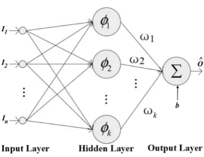
RBFs were introduced into the NN by Broomhead and Lawe in 1988 [9]. The basic form of an RBF network con-sists of three layers the first one is composed of input source nodes that connect the networks to its environment, the second one is hidden layer applies a non-linear trans-formation from the input space to the hidden space and the third one is output layer which consist of linear unit connected to the hidden layer. Using a RBF, the output layer is linear and serves as a summation unit. The struc-ture of a RBF NN with only one output nodes can be given as in Fig. 1.
The number of hidden units usually is larger than the number of networks inputs, so that input space is trans-form into higher dimensional space where become lin-early separable [10].
The RBF network of single output is a non-linear mapping defined as follows:
(1)
where ̂∈R denotes the network output, I is the network input vector, the cis are the location of center of RBFs. ∥⋅∥ denote the norm, ωiis the linear output weight, b repre-sents a bias and k is the number of hidden nodes. There is a large class of RBFs which can be define as:
(2)
(3)
(4)
(5)
Here we used Gaussian basis function which is the most popular and widely used RBF and used by many author in practical applications [11].
(6)
where δ is the width factor of the basis i.
3. Particle Swarm Optimization: Overview
PSO is a population-based optimization algorithm that was developed by Kennedy and Eberhart in 1995 [12]. It was shaped by investigation the behavior of birds and fishes in swarm to find the near optimal solutions. In this algorithm, each bird is called a particle represented as a vector that is a candidate solution [12, 13]. A PSO model is initialized with a swarm of random particles and searches for optima by updating generations.
Assume a D-dimensional searching space. In this search space each particle has two main features: position and velocity. Considering a swarm of N particles seeking for optimum point, position and velocity of each particle rep-resented by Xi=(x1, x2, …, xi) and Vi=(v1, v2, …, vi), re-spectively. Best personal position is also delineated by Pi=(pi1, pi2, …, pid) and Pgis best position among all par-ticles until current step. Velocity and position are updated by the following equations:
(7)
(8)
where ω is inertia weight factor, α1 and α2are the accel-ܱ ൌ σ ߱߶ሺצ ܫ െ ܿצሻ ܾ
ୀଵ
߶ሺצ ܫ െ ܿצሻ ൌ ඥͳ ሺצ ܫ െ ܿצሻଶ
߶ሺצ ܫ െ ܿצሻ ൌ ሺצ ܫ െ ܿצሻଶ݈݊ሺצ ܫ െ ܿצሻ
߶ሺצ ܫ െ ܿצሻ ൌ ͳ ሺצ ܫ െ ܿצሻଶ
߶ሺצ ܫ െ ܿצሻ ൌ ሺצ ܫ െ ܿצሻଷ
߶ሺצ ܫ െ ܿצሻ ൌ ሾെሺצூିצሻమ
ሺఋሻమ ሿ
ݒሺݐ ͳሻ ൌ ݓݒሺݐሻ ߙଵݎଵሾሺݐሻ െ ݔሺݐሻሿ ߙଶݎଶሾሺݐሻ െ ݔሺݐሻሿ
ݔሺݐ ͳሻ ൌ ݔሺݐሻ ݒሺݐ ͳሻ ܱሺ
Fig. 1.Architecture of an RBF network with (n,k,1) structure.
eration coefficients which are used to guide the search be-tween local and social areas in the range of [0, 2]. r1and r2are two independently uniformly distributed random variables in the range of [0, 1].
3. 1. Adaptive Version of PSO
Some research has been done in order to adapt PSO pa-rameters in response to particles status, time and other in-formation about search space. Eberhart and Shi (1998) bring forward inertia weight w and recommend a linearly decreasing relationship between w and generations [14]:
(9)
where wmin, wmax, T and t call as the maximum inertia weight, the minimum inertia weight, the total and the cur-rent number of iterations for the algorithm, respectively. In this equation wminand wmax are set to 0.4 to 0.9, re-spectively. Ref. [15] proposed a random version setting w for dynamic system optimization. Ref. [16] altered Eq. (6) and introduced constriction factor. Other two impor-tant parameters need to be set are acceleration coefficients (α1and α2). Ref. [17] suggested to be set α1 and α2at fixed value of 0.2. Ref. [18] presented linear time-varying ac-celeration coefficients for proposed PSO that result in
equilibrating between local and global searches. This ap-proach improves the algorithm performance and makes it more viable than algorithms with fixed parameters. Ref. [19] considered the acceleration coefficients constant and propose a time varying non-linear function for inertia fac-tor adaptation. Ref. [20] proposed a non-linear time-vary-ing evolution to adapt parameters. In fact, inertia weight and acceleration coefficients values non-linearly decrease or increase according to the current and maximum number of iterations. Ref. [21] defined evolutionary factor by cal-culating mean distance of each particle to all other ones. Their proposed algorithm adapts inertia weight and accel-eration factors considering evolutionary factor. Ref. [22] has pointed out that parameter adaptation can enhance the algorithm performance and lead to improved results.
4. Proposed Method
In order to predict forthcoming DGPS corrections, we gave previous corrections (I(n), I(n-1), …, I(n-p)) to the NN and predict I(n+1), i.e.:
(10)
In other words, NN approximating the function f in an ap-propriately based on the previous data, predict forthcom-ing DGPS correction. Fig. 2 shows architecture of ݓ ൌ ݓ௫െ ݐ
ሺ௪ೌೣି௪ሻ
்
ܱሺ݊ሻ ൌ ݂ሺܫሺ݊ሻǡ ܫሺ݊ െ ͳሻǡ ǥ ǡ ܫሺ݊ െ ሻሻ
Fig. 2.Architecture of proposed RBF NN for DGPS corrections prediction.
proposed RBF NN for DGPS corrections prediction. As Eq. (12), after DGPS correction that is predicted by NN properly is subtracted from value of position domain that is calculated by receiver in order to, result in more accurate and closer to the real position.
(11)
(12)
We improve DGPS accuracy by predicting the future error. Having the predicted value cause more accurate DGPS receiver in case that the receiver has not access to the DGPS correction from station. Moreover, it causes less power consumption.
In many applications all parameters of the RBF NN are optimized by Evolutionary Algorithm (EA) such as PSO, but in this work parameter as well as centers and shape parameter which plays important role in transforming into higher dimensional space for better prediction, is calcu-lated by the average of input data.
By averaging the Gaussian basis function can cover all data in better way. Beside that search space for PSO al-gorithm will reduce, so it works more accurate and faster. Assume that I is input vector so:
c=mean(I) (13)
δ=var(I) (14)
where cis centers and δis shape parameter of RBF NN. The Gaussian RBF method is exponentially or spectrally accurate. The convergence of this method can be discuses in term of two different type of approximation-stationary and non-stationary. In stationary the number of centers is fixed and the shape parameter is refined toward zero. This type of convergence is unique. Non-stationary approxi-mation fixes the values of shape parameter and the num-ber of centers is increased. The error estimates of RBF involve quantity called the fill distance. Geometrically, the fill distance is the radius of the largest possible empty ball that can be placed among the centers in the domain. The Gaussian interpolation convergence to a sufficiently smooth underlying function at a spectral rate as the fill distance diereses. The error estimate of interpolation is [23,24]:
(15)
where his fill distance and kis constant. d(I) is the desired
value and (I) is output of RBFNN. As it shows the spec-tral convergence archives as either fill distance or shape parameter go to zero. Due to this when in procedure of al-gorithm, we take the mean average of data as a center cause decrees of fill distance and this will effect on the spectrally convergence and make the computation accu-rate.
5. Experimental Results
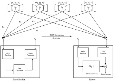
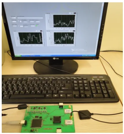
To test the proposed NNs for GPS receivers timing errors prediction a system was built. The test setup was imple-mented and installed on the building of Computer Control and Fuzzy Logic Research Lab in the Iran University of Science and Technology. The observation data received by a low cost and single frequency GPS receiver (1Hz) manufactured by Rockwell Company. The collected data were processed with developed programs by the author’s paper. Fig. 3 shows the data collection system adopted in this research.
Data collection has been at two different times, before and after Selective Availability (S/A). S/A is an intentional degradation of public GPS signals executed for national security reasons by U.S. government. With S/A on, the GPS receiver is confused and doesn't know what is an exact time in satellites, so the S/A forces the satellite to send the unreal time. The time that satellite sends is usu-ally quite close to the real time, but not precise. Without knowing the precise times at the satellites then when they create their time messages, the receiver cannot tell the exact location. Due to that all data was collected under two condition S/A on and off, in regards to have a better
ห݀ሺܫሻ െ ܱሺܫሻห ݇ߟǤഃభͲ ൏ ߟ ൏ ͳ
ܱሺ
݀ݔǡ ݀ݕǡ ݀ݖሺ݊ሻȁ௨௧ௗൌ ݔǡ ݕǡ ݖሺ݊ሻȁோ௩ௗെ
ݔǡ ݕǡ ݖሺ݊ሻȁ௦ௌ௧௧ (
ݔǡ ݕǡ ݖሺ݊ ͳሻȁௗௗൌ ݔǡ ݕǡ ݖሺ݊ ͳሻȁோ௩ௗെ
݀ݔǡ ݀ݕǡ ݀ݖሺ݊ ͳሻȁௗ௧ௗ௬ேே (12)
Fig. 3.Data collection and processing system.
case study and more realistic [25].
In preparing the training data, all input and output vari-ables are normalized in the range [0,1] to reduce the train-ing time [26].
All data were used for prediction in two cases, first one step ahead method and off-line prediction.
5. 1. Prediction with On-line Learning In on-line prediction, data at time t is applied to NNs inputs and the networks must predict the value of instant t +1. The choice of the order for the NNs is very important in on-line prediction. The results demonstrate higher accuracy and more robustness of the proposed PSO based algorithm than
the PSO ones and Back Propagation (BP) [6].
BP stands for backward propagation of errors, is a usual method of training artificial NNs used in relevance with an optimization method such as gradient descent. The method computes the gradient of a fitness function with tribute to all the weights in the network. The gradient is fed to the optimization method which in turn uses it to up-date the weights, in an attempt to minimize the fitness function.
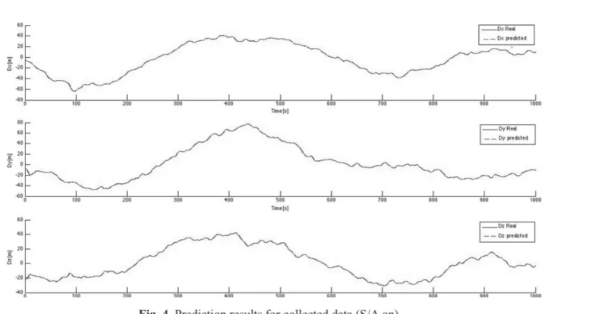
Fig.s 4 and 5 show the original data and the predicted val-ues for both the training data and the test data in S/A on and S/A off, respectively.
Using our algorithm, among 15 runs, the best result is
Fig. 5. Prediction results for collected data (S/A off). Fig. 4. Prediction results for collected data (S/A on).
listed in Tables 1 and 2. To verify the superiority of our proposed method with respect to PSO and BP, Root Mean Square (RMS) error was used as:
(16)
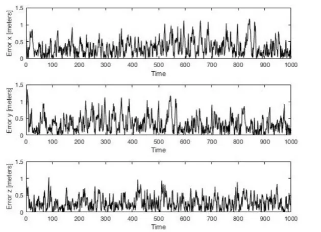
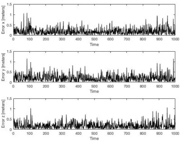
where N is number of tests, diand irepresent the desired coordinates data and RBFNN output data, respectively. Due to accurate prediction in Fig.s 4 and 5, it quite diffi-cult to differ predicted value from original data. In order to that, Fig.s 6 and 7 show the prediction error values in
S/A on and S/A off, respectively.
5. 2. Prediction with Off-line Learning In off-line learning, 70% of the data of data set is used as the train set and the rest is considered as test set to validate the functionality of trained network. The results have been summarized in Tables 3 to 6. The results demonstrate higher accuracy and more robustness of the proposed PSO based algorithm than the PSO ones. Comparison of our computed results with the results reported in [27] show that the accuracy of prediction has been improved twice. Performance of the proposed method was illustrated in comparison with the performance of auto-regression in
ܴܯܵ ൌ ටଵ
ேσ ሺ݀െ ܱሻ ଶ ே
ୀଵ
ܱሺ
Methods RMSx(m) RMSy(m) RMSz(m) RMST(m)
RBFNNtrainedbyBP 0.6798 0.5076 0.5174 0.9937 RBFNNtrainedbyPSO 0.3422 0.3915 0.2829 0.5919 RBFNNtrainedbyproposed
method
0.2929 0.3543 0.2284 0.5133
Table 1.Comparison of test results of different methods for DGPS corrections prediction (on-line training and S/A on).
Methods RMSx(m) RMSy(m) RMSz(m) RMST(m)
RBFNNtrainedbyBP 0.5883 0.7057 0.6660 1.1347 RBFNNtrainedbyPSO 0.1290 0.1651 0.1307 0.2470 RBFNNtrainedbyproposed
method
0.1237 0.1468 0.1214 0.2271
Table 2. Comparison of test results of different methods for DGPS corrections prediction (on-line training and S/A off).
Fig. 6. Prediction errors for position components (S/A on).
[28] and Kalman filter in [6] and was showed in Table 7. As it is evident, the experimental test results with real data emphasize in Table 7 emphasize that RBF NN trained with PSO lead to lower RMS value and also more accu-racy for DGPS corrections prediction.
6. Conclusion
Creating the RBF NNs that solve the problem of DGPS corrections prediction is a difficult task, because many pa-rameters (number of hidden neurons, input variables, cen-ters, width and output layer's weights) have to be set at
Methods RMSx(m) RMSy(m) RMSz(m) RMST(m)
RBFNNtrainedbyPSO 0.0393 0.0523 0.0902 0.1143
RBFNNtrainedbyproposed
method 0.0203 0.0190 0.0423 0.0506
Table 3. Comparison of test results of different method for GPS errors prediction (training and S/A on).
Methods RMSx(m) RMSy(m) RMSz(m) RMST(m)
RBFNNtrainedbyPSO 0.0338 0.0721 0.1242 0.1476
RBFNNtrainedby
proposedmethod 0.0197 0.0148 0.0327 0.0410 Table 4. Comparison of test results of different Method for GPS errors prediction (test and S/A on).
Methods RMSx(m) RMSy(m) RMSz(m) RMST(m)
RBFNNtrainedbyPSO 0.0718 0.0380 0.0575 0.0995 RBFNNtrainedby
proposedmethod 0.0704 0.0309 0.0550 0.0945 Table 5. Comparison of test results of different Method for GPS errors prediction (training and S/A off).
Fig. 7. Prediction errors for position components (S/A off).
the same time. This paper proposed a novel EA to deter-mine network parameters (weights) of RBF NNs simul-taneously. Our proposed algorithm generated a new way to determine network parameters such as centers and shape parameter by using averaging of input data. To eval-uate the performance of proposed algorithm, it was com-pared with several well-known methods. Simulation results indicated that our model has better prediction ac-curacy with computational efficiency. Moreover, the RMS error of our method is about 0.13 meter. Finally, a real world case study was presented. The proposed method was applied to predict GPS errors. Also, the obtained re-sults were compared with the basic PSO which verified the superiority of our proposed method.
References
[1] A. V. Bagrov, V. A. Leonov, A. S. Mitkin, A. F. Nasyrov, A. D. Ponomarenko, K. M. Pichkhadze and V. K. Sysoev, “Single-Satellite Global Posi-tioning System”, Acta Astronautica, vol. 117, pp. 332-337, 2015.
[2] M. Shaw, K. Sandhoo and D. Turner, “ Moderniza-tion of the Global PosiModerniza-tioning System”, Journal of GPS World, vol. 11, no. 9, pp. 36-44, 2000. [3] M. R. Azarbad and M. R. Mosavi, “A New Method
to Mitigate Multipath Error in Single- Frequency GPS Receiver with Wavelet Transform”, Journal of GPS Solutions, vol. 18, no. 2, pp. 189-198, 2014. [4] M. R. Mosavi, S. Azarshahi, I. EmamGholipour
and A. A. Abedi, “Least Squares Techniques for GPS Receivers Positioning Filter using Pseudo-range and Carrier Phase Measurements”, Iranian Journal of Electrical and Electronic Engineering, vol. 10, no. 1, pp. 18-26, 2014.
[5] M. H. Refan, A. Dameshghi and M. Kamarzarrin, “Implementation of DGPS Reference and User Sta-tions Based on RPCE Factors”, Journal of Wireless
Personal Communication, vol. 90, no. 4, pp. 1597-1617, 2016.
[6] M. R. Mosavi, “Comparing DGPS Corrections Prediction using Neural Network, Fuzzy Neural Network and Kalman Filter”, Journal of GPS So-lutions, vol. 10, no. 2, pp. 97-107, 2006.
[7] M. R. Mosavi and H. Nabavi, “Accurate Prediction of DGPS Correction using Neural Network Trained by Imperialistic Competition Algorithm”, Journal of Advances in Computer Research, vol. 6, no. 2, pp. 73-82, 2015.
[8] M. R. Mosavi, “Infrared Counter-Countermeasure Efficient Techniques using Neural Network, Fuzzy System and Kalman Filter”, Iranian Journal of Electrical and Electronic Engineering, vol. 5, no. 4, pp. 215-222, 2009.
[9] D. Broomhead and D. Lowe, “Multivariable Func-tional Interpolation and Adaptive Networks”, Com-plex System, vol. 2, pp. 321-355, 1988.
[10] T. M. Cover, “Geometrical and Statistical Proper-ties of Systems of Linear InequaliProper-ties with Applica-tions in Pattern Recognition”, IEEE Transaction on Industrial Electronic Computation, vol. 3, pp. 326-334, 1965.
[11] R. Neruda and P. Kudovia, “Learning Method for Radial Basis Function Networks”, Future Genera-tion ComputaGenera-tion System, vol. 21, pp. 1131-1142, 2005.
[12] R. C. Eberhart, Y. Shi and J. Kennedy, “Swarm In-telligence”, Morgan Kaufmann, 2001.
[13] J. Kennedy and R. C. Eberhart, “A Discrete Binary Version of the Particle Swarm Algorithm”, IEEE Conference on Systems, Man, and Cybernetics, Computational Cybernetics and Simulation, vol. 5, pp. 4104-4108, 1997.
[14] R. C. Eberhart and Y. Shi, “A Modified Particle Swarm Optimizer”, IEEE Congress on
Computa-Methods RMSx(m) RMSy(m) RMSz(m) RMST(m)
RBFNNtrainedbyPSO 0.0725 0.0370 0.0531 0.0972
RBFNNtrainedby
proposedmethod 0.0713 0.0311 0.0491 0.0921 Table 6. Comparison of test results of different Method for GPS errors prediction (test and S/A off).
basedalgorithmthanthePSOones. Comparisonof
Methods TotalRMSError
(inmeters) Autoregression [28] 1.0848
Kalmanfilter [6] 0.5861 Proposedmethod
(RBFNN)
0.2271
Table 7. Accuracy of DGPS corrections prediction using autoregression, Kalman filter and RBF NN with SA off
tional Intelligence, pp. 69-73, 1998.
[15] R. C. Eberhart and Y. Shi, “Tracking and Optimiz-ing Dynamic Systems with Particle Swarms”, IEEE Congress on Evolutionary Computation, vol. 1, pp. 94-100, 2001.
[16] M. Clerc and J. Kennedy, “The Particle Swarm-Ex-plosion, Stability and Convergence in a Multidi-mensional Complex Space”, IEEE Transaction on Evolutionary Computation, vol. 6, pp. 58-73, 2002. [17] J. Kennedy and R. Eberhart, “Particle Swarm Op-timization”, IEEE International Conference on Neural Networks, vol. 4, pp. 1942-1948, 1995. [18] A. Ratnaweera, S. Halgamuge and H. Watson,
“Self-Organizing Hierarchical Particle Swarm Op-timizer with Time-Varying Acceleration Coeffi-cients”, IEEE Transaction on Evolutionary Computation, vol. 8, pp. 240-255, 2004.
[19] A. Chatterjee and P. Siarry, “Nonlinear Inertia Weight Variation for Dynamic Adaptation in Parti-cle Swarm Optimization”, Computation Opera-tional Research, vol. 33, pp. 859-871, 2006. [20] C. N. Ko, Y. P. Chang and C. J. Wu, “An
Orthogo-nal-Array-based Particle Swarm Optimizer with Nonlinear Time-Varying Evolution”, Applied Math-ematical Computation, vol. 191, pp. 272-279, 2007. [21] Z. H. Zhan, J. Zhang, Y. Li and H. H. Chung,
“Adaptive Particle Swarm Optimization”, IEEE Transaction System on Man Cybernetic Part B: Cy-bernetic, vol. 39, pp. 1362-1381, 2009.
[22] M. Clerc, “Particle Swarm Optimization”, Wiley-ISTE, London, 2010.
[23] M. Buhmann and N. Dyn, “Spectral Convergence of Multiquadric Interpolation”, Proceedings of the Edinburgh Mathematical Society, vol. 36, pp. 319-333, 1993.
[24] W. R. Madych and S. A. Nelson, “Bounds on Mul-tivariate Polynomials and Exponential Error Esti-mates for Multiquadric Interpolation”, Journal of Approximation Theory, vol. 70, pp. 94-114, 1992. [25] M. R. Mosavi, K. Mohammadi and M. H. Refan, “A New Approach for Improving of GPS Position-ing Accuracy usPosition-ing an Adaptive Neurofuzzy System, before and after S/A Is Turned off”, Journal of En-gineering Science, Iran University of Science and Technology, vol. 15, no. 1, pp. 101-114, 2004. [26] M. R. Mosavi, “Precise Real-Time Positioning with
a Low Cost GPS Engine using Neural Networks”, Journal of Survey Review, vol.39, no.306, pp.316-327, 2007.
[27] M. H. Refan, A. Dameshghi and M. Kamarzarrin, “Utilizing Hybrid Recurrent Neural Network and Genetic Algorithm for Predicting the Pseudo-Range Correction Factors to Improve the Accuracy of RTDGPS”, Gyroscopy and Navigation, vol. 6, no. 3, pp. 197-206, 2015.
[28] M. R. Mosavi, K. Mohammadi and M. H. Refan, “Time varying ARMA Processing on GPS Data to Improve Positioning Accuracy”, The Asian GPS Conference 2002, India, pp. 125-128, 24-25 Octo-ber 2002.
M. R. Mosavi received his B.S., M.S., and Ph.D. degrees in Electronic Engineering from Iran University of Sci-ence and Technology (IUST), Tehran, Iran in 1997, 1998, and 2004, respectively. He is currently faculty member (professor) of the Department of Electrical Engi-neering of IUST. He is the author of more than 300 scientific publications in journals and international conferences. His research interests include circuits and systems design.
A. Rashidinia received his M.S. degree in Electronic En-gineering from IUST in 2015. His research interests include digital systems and signal pro-cessing.