Challenges of Big Data analysis

Advance access publication 6 February 2014

COMPUTER SCIENCE

Challenges of Big Data analysis

Jianqing Fan

, Fang Han

and Han Liu

1_{Department of} Operations Research and Financial Engineering, Princeton University, Princeton, NJ 08544, USA and 2_{Department of} Biostatistics, Johns Hopkins University, Baltimore, MD 21205, USA ∗_{Corresponding} author.E-mail: jqfan@princeton. edu Received3 August 2013;Accepted15 October 2013

ABSTRACT

Big Data bring new opportunities to modern society and challenges to data scientists. On the one hand, Big Data hold great promises for discovering subtle population patterns and heterogeneities that are not possible with small-scale data. On the other hand, the massive sample size and high dimensionality of Big Data introduce unique computational and statistical challenges, including scalability and storage bottleneck, noise accumulation, spurious correlation, incidental endogeneity and measurement errors. These challenges are distinguished and require new computational and statistical paradigm. This paper gives overviews on the salient features of Big Data and how these features impact on paradigm change on statistical and computational methods as well as computing architectures. We also provide various new perspectives on the Big Data analysis and computation. In particular, we emphasize on the viability of the sparsest solution in high-confidence set and point out that exogenous assumptions in most statistical methods for Big Data cannot be validated due to incidental endogeneity. They can lead to wrong statistical inferences and consequently wrong scientific conclusions.

Keywords:

INTRODUCTION

Big Data promise new levels of scientific discovery and economic value. What is new about Big Data and how they differ from the traditional small- or medium-scale data? This paper overviews the oppor-tunities and challenges brought by Big Data, with emphasis on the distinguished features of Big Data and statistical and computational methods as well as computing architecture to deal with them.

BACKGROUND

We are entering the era of Big Data—a term that refers to the explosion of available information. Such a Big Data movement is driven by the fact that mas-sive amounts of very high-dimensional or unstruc-tured data are continuously produced and stored with much cheaper cost than they used to be. For example, in genomics we have seen a dramatic drop in price for whole genome sequencing [1]. This is also true in other areas such as social media analysis, biomedical imaging, high-frequency finance, analy-sis of surveillance videos and retail sales. The

ex-isting trend that data can be produced and stored more massively and cheaply is likely to maintain or even accelerate in the future [2]. This trend will have deep impact on science, engineering and busi-ness. For example, scientific advances are becom-ing more and more data-driven and researchers will more and more think of themselves as consumers of data. The massive amounts of high-dimensional data bring both opportunities and new challenges to data analysis. Valid statistical analysis for Big Data is becoming increasingly important.

GOALS AND CHALLENGES

OF ANALYZING BIG DATA

What are the goals of analyzing Big Data? According to [3], two main goals of high-dimensional data anal-ysis are to develop effective methods that can accu-rately predict the future observations and at the same time to gain insight into the relationship between the features and response for scientific purposes. Fur-thermore, due to large sample size, Big Data give rise to two additional goals: to understand heterogeneity

C

The Author 2014. Published by Oxford University Press on behalf of China Science Publishing & Media Ltd. All rights reserved. For Permissions, please email: journals. [email protected]

and commonality across different subpopulations. In other words, Big Data give promises for: (i) ex-ploring the hidden structures of each subpopulation of the data, which is traditionally not feasible and might even be treated as ‘outliers’ when the sample size is small; (ii) extracting important common fea-tures across many subpopulations even when there are large individual variations.

What are the challenges of analyzing Big Data? Big Data are characterized by high dimensionality and large sample size. These two features raise three unique challenges: (i) high dimensionality brings noise accumulation, spurious correlations and inci-dental homogeneity; (ii) high dimensionality com-bined with large sample size creates issues such as heavy computational cost and algorithmic instabil-ity; (iii) the massive samples in Big Data are typi-cally aggregated from multiple sources at different time points using different technologies. This creates issues of heterogeneity, experimental variations and statistical biases, and requires us to develop more adaptive and robust procedures.

PARADIGM SHIFTS

To handle the challenges of Big Data, we need new statistical thinking and computational methods. For example, many traditional methods that perform well for moderate sample size do not scale to massive data. Similarly, many statistical methods that per-form well for low-dimensional data are facing signif-icant challenges in analyzing high-dimensional data. To design effective statistical procedures for explor-ing and predictexplor-ing Big Data, we need to address Big Data problems such as heterogeneity, noise accumu-lation, spurious correlations and incidental endor-geneity, in addition to balancing the statistical accu-racy and computational efficiency.

In terms of statistical accuracy, dimension reduc-tion and variable selecreduc-tion play pivotal roles in an-alyzing high-dimensional data. This is designed to address noise accumulation issues. For example, in high-dimensional classification, [4] and [5] showed that conventional classification rules using all fea-tures perform no better than random guess due to noise accumulation. This motivates new regulariza-tion methods [6–10] and sure independence screen-ing [11–13]. Furthermore, high dimensionality in-troduces spurious correlations between response and unrelated covariates, which may lead to wrong statistical inference and false scientific conclusions [14]. High dimensionality also gives rise to inci-dental endogeneity, a phenomenon that many unre-lated covariates may incidentally be correunre-lated with the residual noises. The endogeneity creates statisti-cal biases and causes model selection inconsistency

that lead to wrong scientific discoveries [15,16]. Yet, most statistical procedures are based on unrealistic exogenous assumptions that cannot be validated by data (see the ‘Incidental endogeneity’ section and [17]). New statistical procedures with these issues in mind are crucially needed.

In terms of computational efficiency, Big Data motivate the development of new computational in-frastructure and data-storage methods. Optimiza-tion is often a tool, not a goal, to Big Data analy-sis. Such a paradigm change has led to significant progresses on developments of fast algorithms that are scalable to massive data with high dimension-ality. This forges cross-fertilizations among differ-ent fields including statistics, optimization and ap-plied mathematics. For example, the authors of [18] showed that the non-deterministic polynomial-time hard (NP-hard) best subset regression can be re-cast as an L1-norm penalized least-squares prob-lem which can be solved by the interior point method. Alternative algorithms to accelerate this

L1-norm penalized least-squares problems, such as least angle regression [19], threshold gradient de-scent [20] and coordinate dede-scent [21,22], itera-tive shrinkage-thresholding algorithms [23,24], are proposed. Besides large-scale optimization algo-rithms, Big Data also motivate the development of majorization–minimization algorithms [25–27], ‘large-scale screening and small-scale optimization’ framework [28], parallel computing methods [29– 31] and approximate algorithms that are scalable to large sample size.

ORGANIZATION OF THIS PAPER

The rest of this paper is organized as follows. The section ‘Rises of Big Data’ overviews the rise of Big Data problem from science, engineering and social science. The ‘Salient Features of Big Data’ section ex-plains some unique features of Big Data and their im-pacts on statistical inference. Statistical methods that tackle these Big Data problems are given in the ‘Im-pact on statistical thinking’ section. The ‘Im‘Im-pact on computing infrastructure’ section gives an overview on scalable computing infrastructure for Big Data storage and processing. The ‘Impact on computa-tional methods’ section discusses the computacomputa-tional aspect of Big Data and introduces some recent pro-gresses. The ‘Conclusions and future perspectives’ section concludes the paper.

RISE OF BIG DATA

Massive sample size and high dimensionality char-acterize many contemporary datasets. For example,

in genomics, there have been more than 500 000 mi-croarrays that are publicly available with each array containing tens of thousands of expression values of molecules; in biomedical engineering, there have been tens of thousands of terabytes of functional magnetic resonance images (fMRIs) with each im-age containing more than 50 000 voxel values. Other examples of massive and high-dimensional data in-clude unstructured text corpus, social medias, and fi-nancial time series, e-commerce data, retail transac-tion records and surveillance videos. We now briefly illustrate some of these Big Data problems.

Genomics

Many new technologies have been developed in ge-nomics and enable inexpensive and high-throughput measurement of the whole genome and transcrip-tome. These technologies allow biologists to gen-erate hundreds of thousands of datasets and have shifted their primary interests from the acquisition of biological sequences to the study of biological function. The availability of massive datasets sheds light towards new scientific discoveries. For exam-ple, the large amount of genome sequencing data now make it possible to uncover the genetic mark-ers of rare disordmark-ers [32,33] and find associations be-tween diseases and rare sequence variants [34,35]. The breakthroughs in biomedical imaging technol-ogy allow scientists to simultaneously monitor many gene and protein functions, permitting us to study interactions in regulatory processes and neuron ac-tivities. Moreover, the emergence of publicly avail-able genomic databases enavail-ables integrative analysis which combines information from many sources for drawing scientific conclusions. These research stud-ies give rise to many computational methods as well as new statistical thinking and challenges [36].

One of the important steps in genomic data anal-ysis is to remove systematic biases (e.g. intensity ef-fect, batch efef-fect, dye efef-fect, block efef-fect, among oth-ers). Such systematic biases are due to experimental variations, such as environmental, demographic, and other technical factors, and can be more severe when we combine different data sources. They have been shown to have substantial effects on gene expression levels, and failing to taking them into consideration may lead to wrong scientific conclusions [37]. When the data are aggregated from multiple sources, it re-mains an open problem on what is the best normal-ization practice.

Even with the systematic biases removed, an-other challenge is to conduct large-scale tests to pick important genes, proteins, or single-nucleotide poly-morphism (SNP). In testing the significance of

thou-sands of genes, classical methods of controlling the probability of making one falsely discovered gene are no longer suitable and alternative procedures have been designed to control the false discovery rates [38–42] and to improve the power of the tests [42]. These technologies, though high-throughput in measuring the expression levels of tens of thou-sands of genes, remain low-throughput in surveying biological contexts (e.g. novel cell types, tissues, dis-eases, etc.).

An additional challenge in genomic data analy-sis is to model and explore the underlying hetero-geneity of the aggregated datasets. Due to technol-ogy limitations and resource constraints, a single lab usually can only afford performing experiments for no more than a few cell types. This creates a ma-jor barrier for comprehensively characterizing gene regulation in all biological contexts, which is a fun-damental goal of functional genomics. On the other hand, the National Center for Biotechnology Infor-mation (NCBI) Gene Expression Omnibus (GEO) [43] and other public databases have cumulated more than 500 000 gene expression profiles, includ-ing microarray, exon array and ribonucleic acid-sequencing (RNA-seq) samples from thousands of biological contexts. Public ChIP–chip and ChIP– seq data generated by different labs for different pro-teins and in different contexts are also steadily grow-ing. Together, these public data contain enormous amounts of information that have not been fully ex-ploited so far. Massive data aggregated from these public databases shed light on systematically study-ing many biological contexts in a high-throughput way. However, how to systematically explore the un-derlying heterogeneity and unveil the commonal-ity across different subpopulations remains an active research area.

Neuroscience

Many important diseases, including Alzheimer’s dis-ease, Schizophrenia, Attention Deficit Hyperactive Disorder, Depression and Anxiety, have been shown to be related to brain connectivity networks. Under-standing the hierarchical, complex, functional net-work organization of the brain is a necessary first step to explore how the brain changes with disease. Rapid advances in neuroimaging techniques, such as fMRI and positron emission tomography as well as electro-physiology, provide great potential for the study of functional brain networks, i.e. the coherence of the activities among different brain regions [44].

Take fMRI for example. It is a non-invasive tech-nique for determining the neural correlates of men-tal processes in humans. During the past decade, this

technique has become a leading method in the fields of cognitive and physiological neuroscience and kept producing massive amounts of high-resolution brain images. These images enable us to explore the asso-ciation between brain connectivity and potential re-sponses such as disease or psychological status. The fMRI data are massive and very high dimensional. Due to its non-invasive feature, everyday many fMRI machines keep scanning different subjects and con-stantly produce new imaging data. For each data point, the subject’s brain is scanned for hundreds of times. Therefore, it is a 3D time-course image which contains more than hundreds of thousands of voxels. At the same time, the fMRI images are noisy due to its technological limit and possible head motion of the subjects. Analyzing such high-dimensional and noisy data poses great challenges to statisticians and neuroscientists.

Similar to the field of genomics, an important Big Data problem in neuroscience is to aggregate datasets from multiple sources. Brain imaging data sharing is becoming more and more frequent nowa-days [45]. Primary sources of fMRI data arise from the International Data Sharing Initiative and the 1000 Functional Connectomes Project [46], Autism Brain Imaging Data Exchange (ABIDE) [47] and ADHD-200 [48] datasets. These international ef-forts have compiled thousands of resting-state fMRI scans along with complimentary structural scans. The largest of the datasets is the 1000 Functional Connectomes Project, which focuses on healthy adults and includes limited covariate information on age, gender, handedness and image quality. The ADHD-200 dataset is similarly structured; yet, it includes diagnostic information on disease status such as human IQ. The ABIDE dataset is similar to the ADHD-200 dataset, with diagnostic autism and symptom severity information. However, it has a greater balance between diseased and non-diseased subjects. These large datasets pose great opportuni-ties as well as new challenges.

One of the main challenges, as in the area of ge-nomics, is to remove the systematic biases caused by experimental variations and data aggregations. Moreover, statistically controlled inclusion of a sub-ject in a group study, i.e. testing whether a per-son should be rejected as outlier data, is often poorly conducted [49] and voxels cannot be per-fectly aligned across different experiments in differ-ent laboratories. Therefore, the collected data con-tain many outliers and missing values. These is-sues make data preprocessing and analysis signifi-cantly more complicated. Many traditional statisti-cal procedures are not well suited in this noisy high-dimensional settings, and new statistical thinking is crucially needed.

Economics and finance

Over the past decade, more and more corpora-tions are adopting the data-driven approach to con-duct more targeted services, reduce risks and im-prove performance. They are implementing special-ized data analytics programs to collect, store, man-age and analyze large datasets from a range of sources to identify key business insights that can be ploited to support better decision making. For ex-ample, available financial data sources include stock prices, currency and derivative trades, transaction records, high-frequency trades, unstructured news and texts, consumers’ confidence and business sen-timents buried in social media and internet, among others. Analyzing these massive datasets helps mea-suring firms risks as well as systematic risks. It re-quires professionals who are familiar with sophis-ticated statistical techniques in portfolio manage-ment, securities regulation, proprietary trading, fi-nancial consulting and risk management.

Analyzing a large panel of economic and finan-cial data is challenging. For example, as an impor-tant tool in analyzing the joint evolution of macroe-conomics time series, the conventional vector au-toregressive (VAR) model usually includes no more than 10 variables, given the fact that the number of parameters grows quadratically with the size of the model. However, nowadays econometricians need to analyze multivariate time series with more than hundreds of variables. Incorporating all information into the VAR model will cause severe overfitting and bad prediction performance. One solution is to re-sort to sparsity assumptions, under which new sta-tistical tools have been developed [50,51].

Another example is portfolio optimization and risk management [52,53]. In this problem, estimat-ing the covariance and inverse covariance matrices of the returns of the assets in the portfolio plays an im-portant role. Suppose that we have 1000 stocks to be managed. There are 500 500 covariance parameters to be estimated. Even if we could estimate each indi-vidual parameter accurately, the cumulated error of the whole matrix estimation can be large under ma-trix norms. This requires new statistical procedures. See, for example, [54–66] on estimating large covari-ance matrices and their inverse.

Other applications

Big Data have numerous other applications. Tak-ing social network data analysis for example, mas-sive amount of social network data are being produced by Twitter, Facebook, LinkedIn and YouTube. These data reveal numerous individual’s characteristics and have been exploited in various

fields. For example, the authors of [67] used these data to predict influenza epidemic; those of [68] used these data to predict the stock mar-ket trend; and the authors of [69] used the so-cial network data to predict box-office revenues for movies. In addition, the social media and Internet contain massive amount of information on the consumer preferences and confidences, leading economics indicators, business cycles, political atti-tudes, and the economic and social states of a soci-ety. It is anticipated that the social network data will continue to explode and be exploited for many new applications.

Several other new applications that are becoming possible in the Big Data era include:

(i) Personalized services. With more personal data collected, commercial enterprises are able to provide personalized services adapt to individ-ual preferences. For example, Target (a retail-ing company in the United States) is able to predict a customer’s need by analyzing the col-lected transaction records.

(ii) Internet security.When a network-based attack takes place, historical data on network traffic may allow us to efficiently identify the source and targets of the attack.

(iii) Personalized medicine.More and more health-related metrics such as individual’s molecular characteristics, human activities, human habits and environmental factors are now available. Using these pieces of information, it is possi-ble to diagnose an individual’s disease and se-lect individualized treatments.

(iv) Digital humanities. Nowadays many archives are being digitized. For example, Google has scanned millions of books and identified about every word in every one of those books. This produces massive amount of data and enables addressing topics in the humanities, such as mapping the transportation system in ancient Roman, visualizing the economic connections of ancient China, studying how natural lan-guages evolve over time, or analyzing historical events.

SALIENT FEATURES OF BIG DATA

Big Data create unique features that are not shared by the traditional datasets. These features pose sig-nificant challenges to data analysis and motivate the development of new statistical methods. Unlike tra-ditional datasets where the sample size is typically larger than the dimension, Big Data are character-ized by massive sample size and high dimensional-ity. First, we will discuss the impact of large sam-ple size on understanding heterogeneity: on the one

hand, massive sample size allows us to unveil hidden patterns associated with small subpopulations and weak commonality across the whole population. On the other hand, modeling the intrinsic heterogene-ity of Big Data requires more sophisticated statistical methods. Secondly, we discuss several unique phe-nomena associated with high dimensionality, includ-ing noise accumulation, spurious correlation and in-cidental endogeneity. These unique features make traditional statistical procedures inappropriate. Un-fortunately, most high-dimensional statistical tech-niques address only noise accumulation and spuri-ous correlations issues, but not incidental endogene-ity. They are based on exogeneity assumptions that often cannot be validated by collected data, due to incidental endogeneity.

Heterogeneity

Big Data are often created via aggregating many data sources corresponding to different subpopulations. Each subpopulation might exhibit some unique fea-tures not shared by others. In classical settings where the sample size is small or moderate, data points from small subpopulations are generally categorized as ‘outliers’, and it is hard to systematically model them due to insufficient observations. However, in the Big Data era, the large sample size enables us to better understand heterogeneity, shedding light to-ward studies such as exploring the association be-tween certain covariates (e.g. genes or SNPs) and rare outcomes (e.g. rare diseases or diseases in small populations) and understanding why certain treat-ments (e.g. chemotherapy) benefit a subpopulation and harm another subpopulation. To better illus-trate this point, we introduce the following mixture model for the population:

λ1p1(y;θ1(x))+ · · · +λmpm(y;θm(x)), (1)

whereλj≥0 represents the proportion of thejth

subpopulation, pj

y;θj(x)

is the probability dis-tribution of the response of thejth subpopulation given the covariatesxwithθj(x) as the parameter

vector. In practice, many subpopulations are rarely observed, i.e.λjis very small. When the sample size nis moderate,nλjcan be small, making it infeasible

to infer the covariate-dependent parametersθj(x)

due to the lack of information. However, because Big Data are characterized by large sample sizen, the sample sizenλjfor thejth subpopulation can be

moderately large even ifλj is very small. This

en-ables us to more accurately infer about the subpop-ulation parametersθj(·). In short, the main

advan-tage brought by Big Data is to understand the het-erogeneity of subpopulations, such as the benefits of

certain personalized treatments, which are infeasible when sample size is small or moderate.

Big Data also allow us to unveil weak common-ality across whole population, thanks to large sam-ple sizes. For examsam-ple, the benefit of one drink of red wine per night on heart can be difficult to assess without large sample size. Similarly, health risks to exposure of certain environmental factors can only be more convincingly evaluated when the sample sizes are sufficiently large.

Besides the aforementioned advantages, the het-erogeneity of Big Data also poses significant chal-lenges to statistical inference. Inferring the mix-ture model in (1) for large datasets requires so-phisticated statistical and computational methods. In low dimensions, standard techniques such as the expectation–maximization algorithm for finite mix-ture models can be applied. In high dimensions, however, we need to carefully regularize the estimat-ing procedure to avoid overfittestimat-ing or noise accumu-lation and to devise good computation algorithms [70,71].

Noise accumulation

Analyzing Big Data requires us to simultaneously es-timate or test many parameters. These estimation er-rors accumulate when a decision or prediction rule depends on a large number of such parameters. Such a noise accumulation effect is especially severe in high dimensions and may even dominate the true signals. It is usually handled by the sparsity assump-tion [2,72,73].

Take high-dimensional classification for in-stance. Poor classification is due to the existence of many weak features that do not contribute to the reduction of classification error [4]. As an example, we consider a classification problem where the data come from two classes:

X1, . . . ,Xn∼Nd(μ1,Id)

andY1, . . . ,Yn∼Nd(μ2,Id). (2)

We want to construct a classification rule which clas-sifies a new observationZ∈Rd_{into either the first}

or the second class. To illustrate the impact of noise accumulation in classification, we setn=100 and

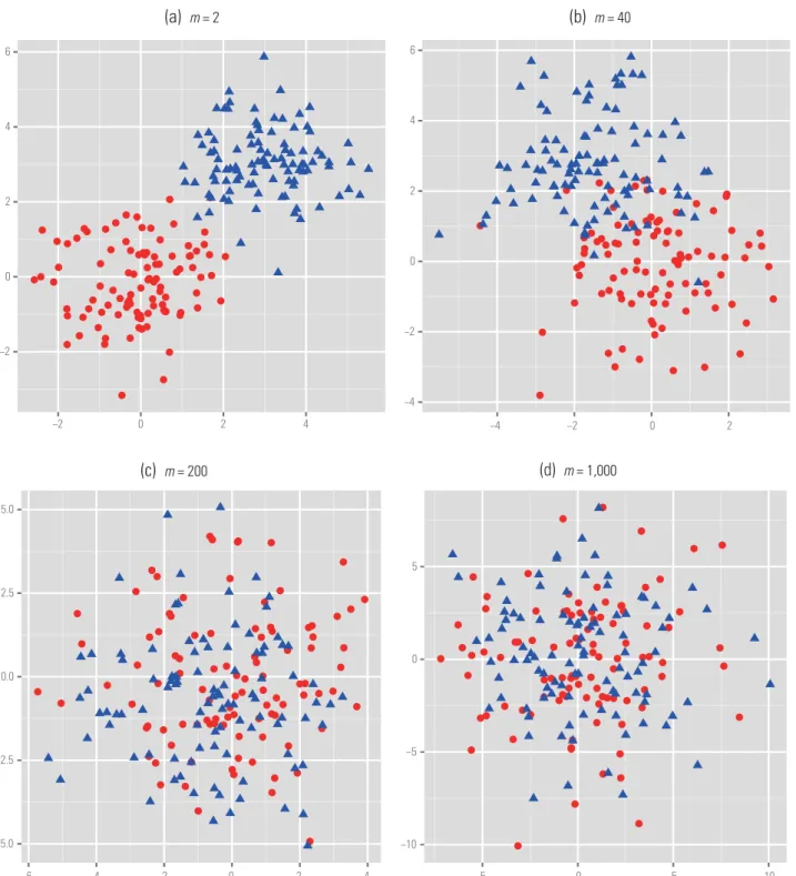
d=1000. We setμ1=0andμ2to be sparse, i.e. only the first 10 entries ofμ2are nonzero with value 3, and all the other entries are zero. Figure 1 plots the first two principal components by using the first

m=2, 40, 200 features and the whole 1000 features. As illustrated in these plots, whenm=2 we obtain high discriminative power. However, the discrimi-native power becomes very low whenmis too large

due to noise accumulation. The first 10 features con-tribute to classifications and the remaining features do not. Therefore, whenm>10, procedures do not obtain any additional signals, but accumulate noises: the larger them, the more the noise accumulates, which deteriorates the classification procedure with dimensionality. Form=40, the accumulated signals compensate the accumulated noise, so that the first two principal components still have good discrimi-native power. Whenm=200, the accumulated noise exceeds the signal gains.

The above discussion motivates the usage of sparse models and variable selection to overcome the effect of noise accumulation. For example, in the classification model (2), instead of using all the features, we could select a subset of features which attain the best signal-to-noise ratio. Such a sparse model provides more improved classification per-formance [72,73]. In other words, variable selec-tion plays a pivotal role in overcoming noise ac-cumulation in classification and regression predic-tion. However, variable selection in high dimensions is challenging due to spurious correlation, inciden-tal endorgeneity, heterogeneity and measurement errors.

Spurious correlation

High dimensionality also brings spurious correla-tion, referring to the fact that many uncorrelated ran-dom variables may have high sample correlations in high dimensions. Spurious correlation may cause false scientific discoveries and wrong statistical infer-ences.

Consider the problem of estimating the coeffi-cient vectorβof a linear model

y=Xβ+, Var()=σ2Id, (3)

wherey∈Rn represents the response vector,X=

[x1, . . . ,xn]T∈Rn×drepresents the design matrix,

∈Rn _{represents an independent random noise}

vector andIdis thed×didentity matrix. To cope

with the noise accumulation issue, when the dimen-siondis comparable to or larger than the sample sizen, it is popular to assume that only a small num-ber of variables contribute to the response, i.e.βis a sparse vector. Under this sparsity assumption, vari-able selection can be conducted to avoid noise accu-mulation, improve the performance of prediction, as well as enhance the interpretability of the model with parsimonious representation.

In high dimensions, even for a model as simple as (3), variable selection is challenging due to the presence of spurious correlation. In particular, [11] showed that, when the dimensionality is high, the

Figure 1.Scatter plots of projections of the observed data (n=100 from each class) onto the first two principal components of the bestm-dimensional selected feature space. A projected data with the filled circle indicates the first class and the filled triangle indicates the second class.

important variables can be highly correlated with several spurious variables which are scientifically unrelated. We consider a simple example to illustrate this phenomenon. Let x1, . . . ,xn be n

indepen-dent observations of ad-dimensional Gaussian ran-dom vectorX=(X1, . . . ,Xd)T ∼Nd(0,Id). We

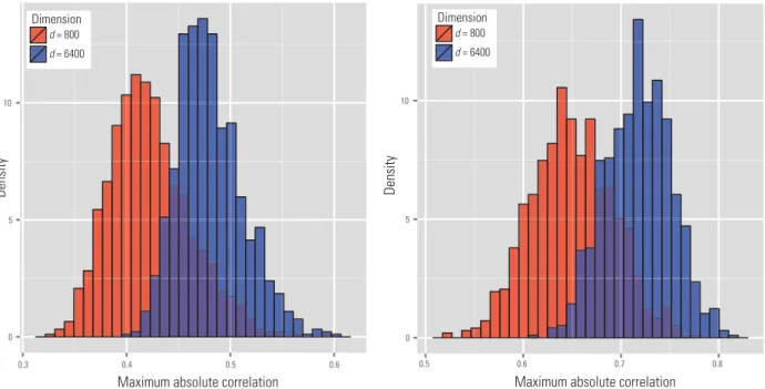
repeatedly simulate the data withn=60 andd=800

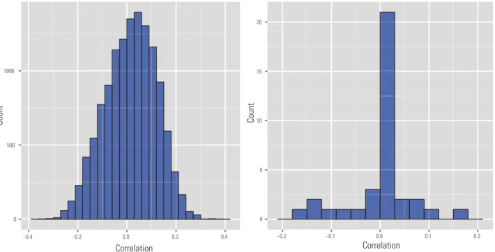
and 6400 for 1000 times. Figure 2a shows the em-pirical distribution of the maximum absolute sample correlation coefficient between the first variable with the remaining ones defined as

r =max j≥2| CorrX1,Xj |, (4)

Figure 2.Illustration of spurious correlation. (a) Distribution of the maximum absolute sample correlation coefficients betweenX1 and{Xj}j=1.

(b) Distribution of the maximum absolute sample correlation coefficients betweenX1and the closest linear projections of any four members of

{Xj}j=1toX1. Here the dimensiondis 800 and 6400, the sample sizenis 60. The result is based on 1000 simulations. where CorrX1,Xj

is the sample correlation between the variablesX1 andXj. We see that the maximum absolute sample correlation becomes higher as dimensionality increases.

Furthermore, we can compute the maximum absolute multiple correlation betweenX1 and lin-ear combinations of several irrelevant spurious variables: R=max |S|=4_{βmaxj}4j=1 Corr ⎛ ⎝X1, j∈S βjXj ⎞ ⎠ . (5) Using the same configuration as in Fig. 2 a, Fig. 2 b plots the empirical distribution of the maximum ab-solute sample correlation coefficient betweenX1and

j∈SβjXj, whereSis any size four subset of{2, ..., d}andβjis the least-squares regression coefficient

ofXjwhen regressingX1on{Xj}j∈S. Again, we see

that even thoughX1is utterly independent ofX2, ...,

Xd, the correlation betweenX1and the closest linear combination of any four variables of{Xj}j=1toX1 can be very high. We refer to [14] and [74] about more theoretical results on characterizing the orders ofr.

The spurious correlation has significant impact on variable selection and may lead to false scientific discoveries. LetXS =(Xj)j∈S be the sub-random

vector indexed bySand letS be the selected set that has the higher spurious correlation withX1as in Fig. 2. For example, whenn=60 andd=6400, we see thatX1is practically indistinguishable fromXS

for a setSwith|S| =4. IfX1represents the expres-sion level of a gene that is responsible for a disease, we cannot distinguish it from the other four genes in Sthat have a similar predictive power although they are scientifically irrelevant.

Besides variable selection, spurious correlation may also lead to wrong statistical inference. We ex-plain this by considering again the same linear model as in (3). Here we would like to estimate the stan-dard errorσ of the residual, which is prominently featured in statistical inferences of regression co-efficients, model selection, goodness-of-fit test and marginal regression. LetSbe a set of selected vari-ables andPSbe the projection matrix on the column

space ofXS. The standard residual variance

estima-tor, based on the selected variables, is σ2₌yT(In−PS)y

n− |S| . (6)

The estimator (6) is unbiased when the variables are not selected by data and the model is correct. However, the situation is completely different when the variables are selected based on data. In particu-lar, the authors of [14] showed that when there are many spurious variables,σ2 _{is seriously} underesti-mated, which leads further to wrong statistical infer-ences including model selection or significance tests, and false scientific discoveries such as finding wrong genes for molecular mechanisms. They also propose a refitted cross-validation method to attenuate the problem.

Incidental endogeneity

Incidental endogeneity is another subtle issue raised by high dimensionality. In a regression setting

Y =d_j=1βjXj+ε, the term ‘endogeneity’ [75]

means that some predictors{Xj}correlate with the

residual noise ε. The conventional sparse model assumes

Y = j

βjXj+ε,

andE(εXj)=0 forj =1, . . . ,d, (7)

with a small setS={j:βj=0}. The exogenous

as-sumption in (7) that the residual noiseεis uncorre-lated with all the predictors is crucial for validity of most existing statistical procedures, including vari-able selection consistency. Though this assumption looks innocent, it is easy to be violated in high di-mensions as some of variables{Xj}are incidentally correlated withε, making most high-dimensional procedures statistically invalid.

To explain the endogeneity problem in more de-tail, suppose that unknown to us, the responseYis related to three covariates as follows:

Y =X1+X2+X3+ε,

with EεXj=0, forj =1,2,3.

In the data-collection stage, we do not know the true model, and therefore collect as many covariates that are potentially related toYas possible, in hope to in-clude all members inSin (7). Incidentally, some of thoseXjs (forj=1, 2, 3) might be correlated with

the residual noiseε. This invalidates the exogenous modeling assumption in (7). In fact, the more co-variates are collected or measured, the harder this assumption is satisfied.

Unlike spurious correlation, incidental endo-geneity refers to the genuine existence of correla-tions between variables unintentionally, both due to high dimensionality. The former is analogous to find two persons look alike but have no genetic relation, whereas the latter is similar to bumping into an ac-quaintance, both easily occurring in a big city. More generally, endogeneity occurs as a result of selection biases, measurement errors and omitted variables. These phenomena arise frequently in the analysis of Big Data, mainly due to two reasons:

r _{With the benefit of new high-throughput}

mea-surement techniques, scientists are able to and tend to collect as many features as possible. This accordingly increases the possibility that some of them might be correlated with the residual noise, incidentally.

r _{Big Data are usually aggregated from multiple}

sources with potentially different data generating

schemes. This increases the possibility of selection bias and measurement errors, which also cause po-tential incidental endogeneity.

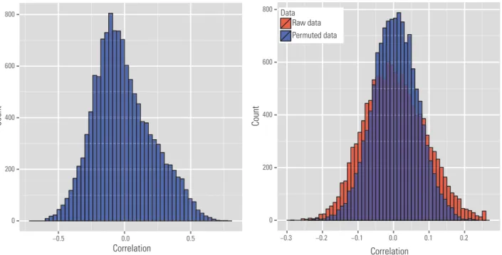
Whether incidental endogeneity appears in real datasets and how shall we test it in practice? We consider a genomics study in which 148 microarray samples are downloaded from GEO database and ArrayExpress [76]. These samples are created un-der the Affymetrix HGU133a platform for human subjects with prostate cancer. The obtained dataset contains 22 283 probes, corresponding to 12 719 genes. In this example, we are interested in the gene named ‘Discoidin domain receptor family, member 1’ (abbreviated as DDR1). DDR1 encodes recep-tor tyrosine kinases, which plays an important role in the communication of cells with their microen-vironment. DDR1 is known to be highly related to the prostate cancer [77] and we wish to study its as-sociation with other genes in patients with prostate cancer. We took the gene expressions of DDR1 as the response variableYand the expressions of all the remaining 12 718 genes as predictors. The left panel of Fig. 3 draws the empirical distribution of the correlations between the response and individual predictors.

To illustrate the existence of endogeneity, we fit anL1-penalized least-squares regression (Lasso) on the data, and the penalty is automatically selected via 10-fold cross validation (37 genes are selected). We then refit an ordinary least-squares regression on the selected model to calculate the residual vector. In the right panel of Fig. 3, we plot the empirical dis-tribution of the correlations between the predictors and the residuals. We see the residual noise is highly correlated with many predictors. To make sure these correlations are not purely caused by spurious corre-lation, we introduce a ‘null distribution’ of the spuri-ous correlations by randomly permuting the orders of rows in the design matrix, such that the predic-tors are indeed independent of the residual noise. By comparing the two distributions, we see that the distribution of correlations between predictors and residual noise on the raw data (labeled ‘raw data’) has a heavier tail than that on the permuted data (labeled ‘permuted data’). This result provides stark evidence of endogeneity in these data.

The above discussion shows that incidental endo-geneity is likely to be present in Big Data. The prob-lem of dealing with endogenous variables is not well understood in high-dimensional statistics. What is the consequence of this endogeneity? The authors of [16] showed that endogeneity causes inconsistency in model selection. In particular, they provided thor-ough analysis to illustrate the impact of endogene-ity on high-dimensional statistical inference and

Figure 3.Illustration of incidental endogeneity on a microarry gene expression data. Left panel: the distribution of the sample correlationCorr(Xj,Y)

(j=1, . . . , 12 718). Right panel: the distribution of the sample correlationCorr(X j,ε). Hereεrepresents the residual noise after the Lasso fit. We

provide the distributions of the sample correlations using both the raw data and permuted data.

proposed alternative methods to conduct linear re-gression with consistency guarantees under weaker conditions. See also the following section.

IMPACT ON STATISTICAL THINKING

As has been shown in the previous section, massive sample size and high dimensionality bring hetero-geneity, noise accumulation, spurious correlation and incidental endogeneity. These features of Big Data make traditional statistical methods invalid. In this section, we introduce new statistical methods that can handle these challenges. For an overview, see [72] and [73].

Penalized quasi-likelihood

To handle the noise-accumulation issue, we assume that the model parameterβas in (3) is sparse. The classical model selection theory, according to [78], suggests to choose a parameter vectorβthat mini-mizes negative penalized quasi-likelihood:

−QL(β)+λβ0, (8)

where QL(β) is the quasi-likelihood ofβand · 0 represents theL0pseudo-norm (i.e. the number of nonzero entries in a vector). Hereλ >0 is a regu-larization parameter that controls the bias-variance tradeoff. The solution to the optimization problem in (8) has nice statistical properties [79]. However,

it is essentially combinatoric optimization and does not scale to large-scale problems.

The estimator in (8) can be extended to a more general form

n(β)+ d

j=1

P_λ,γ(βj), (9)

where the termn(β) measures the goodness of fit

of the model with parameterβandd_j=1Pλ,γ(βj)

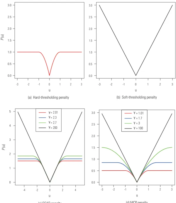
is a sparsity-inducing penalty that encourages spar-sity, in whichλis again the tuning parameter that controls the bias-variance tradeoff andγ is a pos-sible fine-tune parameter which controls the de-gree of concavity of the penalty function [8]. Pop-ular choices of the penalty function P_λ,γ(·) in-clude the hard-thresholding penalty [80,81], soft-thresholding penalty [6,82], smoothly clipped ab-solution deviation (SCAD, [8]) and minimax con-cavity penalty (MCP, [10]). Figure 4 visualizes these penalty functions forλ=1. We see that all penalty functions are folded concave, but the soft-thresholding (L1-)penalty is also convex. The pa-rameterγin SCAD and MCP controls the degree of concavity. From Fig. 4c and d, we see that a smaller value ofγresults in more concave penalties. When

γbecomes larger, SCAD and MCP converge to the soft-thresholding penalty. MCP is a generalization of the hard-thresholding penalty which corresponds to

Figure 4.Visualization of the penalty functions. In all cases,λ=1. For SCAD and MCP, different values ofγare chosen as shown in graphs.

How shall we choose among these penalty func-tions? In applications, we recommend to use either SCAD or MCP thresholding, since they combine the advantages of both hard- and soft-thresholding oper-ators. Many efficient algorithms have been proposed for solving the optimization problem in (9) with the above four penalties. See the ‘Impact on computing infrastructure’ section.

Sparsest solution in high confidence set

The penalized quasi-likelihood estimator (9) is somewhat mysterious. A closely related method is the sparsest solution in high confidence set,

intro-duced in the recent book chapter by [17], which has much better statistical intuition. It is a generally ap-plicable principle that separates the data information and the sparsity assumption.

Suppose that the data information is summarized by the functionn(β) in (9). This can be a

likeli-hood, quasi-likelihood or loss function. The underly-ing parameter vectorβ0usually satisfies(β0)=0, where(·) is the gradient vector of the expected loss function(β)=En(β). Thus, a natural

con-fidence set forβ0is

where·_∞is theL_∞-norm of a vector andγnis

chosen, so that we have confidence level at least 1−

δn, namely

P(β0∈Cn)=P{n(β0)∞≤γn} ≥1−δn.

(11) The confidence setCnis called high-confidence set

sinceδn→0. In theory, we can take any norm in

constructing the high-confidence set. We opt for the

L_∞norm, as it produces a convex confidence setCn

whenn(·) is convex.

The high-confidence set is a summary of the in-formation we have for the parameter vectorβ0. It is not informative in high-dimensional space. Take, for example, the linear model (3) with the quadratic lossn(β)= y−Xβ22. The high-confidence set is then

Cn = {β∈Rd :XT(y−Xβ)∞≤γn},

where we takeγn≥ XTε∞, so thatδn=0. If in

additionβ0is assumed to be sparse, then a natural solution is the intersection of these two pieces of in-formation, namely, finding the sparsest solution in the high-confidence set:

min β∈Cn

β1= min

n(β)∞≤γn

β1. (12)

This is a convex optimization problem when(·) is convex. For the linear model with the quadratic loss, it reduces to the Dantzig selector [9].

There are many flexibilities in defining the spars-est solution in high-confidence set. First of all, we have a choice of the loss functionn(·). We can

re-gard_n(β)=0 as the estimation equations [83] and define directly the high-confidence set (10) from the estimation equations. Secondly, we have many ways to measure the sparsity. For example, we can use a weightedL1-norm to measure the sparsity ofβin (12). By proper choices of estimating equa-tions in (10) and measure of sparsity in (12), the au-thors of [17] showed that many useful procedures can be regarded as the sparsest solution in the high-confidence set. For example, CLIME [84] for esti-mating sparse precision matrix in both the Gaussian graphic model and the linear programming discrim-inant rule [85] for sparse high-dimensional classifi-cation is the sparsest solution in the high-confidence set. The authors of [17] also provided a general vergence theory for such a procedure under a con-dition similar to the restricted eigenvalue concon-dition in [86]. Finally, the idea is applicable to the prob-lems with measurement errors or even endogeneity. In this case, the high-confidence set will be defined accordingly to accommodate the measurement er-rors or endogeneity. See, for example, [87].

Independence screening

An effective variable screening technique based on marginal screening has been proposed by the au-thors of [11]. They aim at handling ultra-high-dimensional data for which the aforementioned pe-nalized quasi-likelihood estimators become compu-tationally infeasible. For such cases, the authors of [11] proposed to first use marginal regression to screen variables, reducing the original large-scale problem to a moderate-scale statistical problem, so that more sophisticated methods for variable selec-tion can be applied. The proposed method, named sure independence screening, is computationally very attractive. It has been shown to possess sure screening property and to have some theoretical ad-vantages over Lasso [13,88].

There are two main ideas of sure independent screening: (i) it uses the marginal contribution of a covariate to probe its importance in the joint model; and (ii) instead of selecting the most impor-tant variables, it aims at removing variables that are not important. For example, assuming each covari-ate has been standardized, we denoteβM

j the

esti-mated regression coefficient in a univariate regres-sion model. The set of covariates that survive the marginal screening is defined as

S= {j :|βM_j | ≥δ} (13) for a given thresholdδ. One can also measure the im-portance of a covariateXjby using its deviance re-duction. For the least-squares problem, both meth-ods reduce to ranking importance of predictors by using the magnitudes of their marginal correlations with the responseY. The authors of [11] and [88] gave conditions under which sure screening prop-erty can be established and false selection rates are controlled.

Since the computational complexity of sure screening scales linearly with the problem size, the idea of sure screening is very effective in the dra-matic reduction of the computational burden of Big Data analysis. It has been extended in various directions. For example, generalized correlation screening was used in [12], nonparametric screening was proposed by [89] and principled sure indepen-dence screening was introduced in [90]. In addition, the authors of [91] utilized the distance correlation to conduct screening, [92] employed rank correla-tion and [28] proposed an iteratively screening and selection method.

Independent screening has never examined the multivariate effect of variables on the response able nor has it used the covariance matrix of vari-ables. An extension of this is to use multivari-ate screening, which examines the contributions of

small groups of variables together. This allows us to examine the synergy of small groups of variables to the response variable. However, the bivariate screen-ing already involvesO(d2_{) submodels, which can} be prohibitive in computation. Covariance assist screening and estimation in [93] can be adapted here to prevent examining all bivariate or multivari-ate submodels. Another possible extension is to de-velop conditional screening techniques, which rank variables according to their conditional contribu-tions given a set of variables.

Dealing with incidental endogeneity

Big Data are prone to incidental endogeneity that makes the most popular regularization methods in-valid. It is accordingly important to develop meth-ods that can handle endogeneity in high dimen-sions. More specifically, let us consider the high-dimensional linear regression model (7). The au-thors of [16] showed that for any penalized estima-tors to be variable selection consistent, a necessary condition is

E(εXj)=0 for j =1, . . . ,d. (14)

As discussed in the ‘Salient features of Big Data’ sec-tion, the condition in (14) is too restrictive for real-world applications. LettingS={j:βj=0}be the set

of important variables, with non-vanishing compo-nents inβ, a more realistic model assumption should be E(ε|{Xj}j∈S)=E Y − j∈S βjXj|{Xj}j∈S =0. (15)

In the paper by the authors of [16], they considered an even weaker version of Equation (15), called the ‘over identification’ condition, such as

EεXj =0 and EεX2j =0 forj ∈S.

(16) Under condition (16), the authors of [16] showed that the classical penalized least-squares methods, such as Lasso, SCAD and MCP, are no longer con-sistent. Instead, they introduced the focused gener-alized methods of moments (FGMMs) by utilizing the over identification conditions and proved that the FGMM consistently selects the set of variables

S. We do not go into the technical details here but illustrate this by an example.

We continue to explore the gene expression data in the ‘Incidental endogeneity’ section. We again treat gene DDR1 as response and other genes as predictors, and apply the FGMM instead of Lasso. By cross validation, the FGMM selects 18 genes. The left panel of Fig. 5 shows the distribu-tion of the sample correladistribu-tions between the genes

Xj(j=1, ... , 12 718) and the residualsεafter the FGMM fit. Here we find that many correlations are nonzero, but it does not matter, because we re-quire only (16). To verify (16), the right panel of Fig. 5 shows the distribution of the sample corre-lations between the 18 selected genes (and their squares) and the residuals. The sample correlations between the selected genes and residuals are zero, and the sample correlations between the squared covariates and residuals are small. Therefore, the modeling assumption is consistent to our model diagnostics.

IMPACT ON COMPUTING

INFRASTRUCTURE

The massive sample size of Big Data fundamentally challenges the traditional computing infrastructure. In many applications, we need to analyze internet-scale data containing billions or even trillions of data points, which even makes a linear pass of the whole dataset unaffordable. In addition, such data could be highly dynamic and infeasible to be stored in a centralized database. The fundamental approach to store and process such data is to divide and conquer. The idea is to partition a large problem into more tractable and independent subproblems. Each sub-problem is tackled in parallel by different process-ing units. Intermediate results from each individual worker are then combined to yield the final output. In small scale, such divide-and-conquer paradigm can be implemented either by multi-core computing or grid computing. However, in very large scale, it poses fundamental challenges to computing infras-tructure. For example, when millions of computers are connected to scale out to large computing tasks, it is quite likely some computers may die during the computing. In addition, given a large computing task, we want to distribute it evenly to many com-puters and make the workload balanced. Design-ing very large scale, high adaptive and fault-tolerant computing systems is extremely challenging and mo-tivates the outcome of new and reliable computing infrastructure that supports massively parallel data storage and processing. In this section, we take Hadoop as an example to introduce basic soft-ware and programming infrastructure for Big Data processing.

Figure 5.Diagnostics of the modeling assumptions of the FGMM on a microarry gene expression data. Left panel: Distribution of the sample correlations

Corr(Xj,ε) (j=1, . . . , 12, 718). Right panel: Distribution of the sample correlationsCorr(X j,ε) andCorr(X2j,ε) for only 18 selected genes. Hereε

represents the residual noise after the FGMM fit.

Hadoop is a Java-based software framework for distributed data management and processing. It contains a set of open source libraries for dis-tributed computing using the MapReduce program-ming model and its own distributed file system called HDFS. Hadoop automatically facilitates scalability and takes cares of detecting and handling failures. Core Hadoop has two key components:

Core Hadoop=Hadoop distributed file system (HDFS)+MapReduce

r _{HDFS is a self-healing, high-bandwidth, clustered}

storage file system, and

r _{MapReduce is a distributed programming model}

developed by Google.

We dart with explaining HDFS and MapReduce in the following two subsections. Besides these two key components, a typical Hadoop release contains many other components. For example, as is shown in Fig. 6, Cloudera’s open-source Hadoop distribu-tion also includes HBase, Hive, Pig, Oozie, Flume and Sqoop. More details about these extra compo-nents are provided in the online Cloudera technical documents. After introducing the Hadoop, we also briefly explain the concepts of cloud computing in the ‘Cloud computing’ section.

Hadoop distributed file system

HDFS is a distributed file system designed to host and provide high-throughput access to large datasets which are redundantly stored across multiple ma-chines. In particular, it ensures Big Data’s durabil-ity to failure and high availabildurabil-ity to parallel applica-tions.

As a motivating application, suppose we have a large data file containing billions of records, and we want to query this file frequently. If many queries are submitted simultaneously (e.g. the Google search engine), the usual file system is not suitable due to the I/O limit. HDFS solves this problem by dividing a large file into small blocks and store them in differ-ent machines. Each machine is called a DataNode. Unlike most block-structured file systems which use Figure 6.An illustration of Cloudera’s open-source Hadoop distribution (source:

Figure 7.An illustration of the HDFS architecture.

a block size on the order of 4 or 8 KB, the default block size in HDFS is 64MB, which allows HDFS to reduce the amount of metadata storage required per file. Furthermore, HDFS allows for fast stream-ing reads of data by keepstream-ing large amounts of data se-quentially laid out on the hard disk. The main trade-off of this decision is that HDFS expects the data to be read sequentially (instead of being read in a ran-dom access fashion).

The data in HDFS can be accessed via a ‘write once and read many’ approach. The metadata struc-tures (e.g. the file names and directories) are allowed to be simultaneously modified by many clients. It is important that this meta information is always syn-chronized and stored reliably. All the metadata are maintained by a single machine, called the NameN-ode. Because of the relatively low amount of meta-data per file (it only tracks file names, permissions and the locations of each block of each file), all such information can be stored in the main memory of the NameNode machine, allowing fast access to the metadata. An illustration of the whole HDFS archi-tecture is provided in Fig. 7.

To access or manipulate a data file, a client con-tacts the NameNode and retrieves a list of locations for the blocks that comprise the file. These loca-tions identify the DataNodes which hold each block. Clients then read file data directly from the DataN-ode servers, possibly in parallel. The NameNDataN-ode is not directly involved in this bulk data transfer, keep-ing its workkeep-ing load to a minimum. HDFS has a built-in redundancy and replication feature which secures that any failure of individual machines can be

recov-ered without any loss of data (e.g. each DataNode has three copies by default). The HDFS automati-cally balances its load whenever a new DataNode is added to the cluster. We also need to safely store the NameNode information by creating multiple redun-dant systems, which allows the important metadata of the file system be recovered even if the NameN-ode itself crashes.

MapReduce

MapReduce is a programming model for processing large datasets in a parallel fashion. We use an exam-ple to explain how MapReduce works. Suppose we are given a symbol sequence (e.g. ‘ATGCCAATC-GATGGGACTCC’), and the task is to write a pro-gram that counts the number of each symbol. The simplest idea is to read a symbol, add it into a hash table with key as the symbol and set value to its num-ber of occurrences. If the symbol is not in the hash table yet, then add the symbol as a new key to the hash and set the corresponding value to 1. If the sym-bol is already in the hash table, then increase the value by 1. This program runs in a serial fashion and the time complexity scales linearly with the length of the symbol sequence. Everything looks simple so far. However, imagine if instead of a simple sequence, we need to count the number of symbols in the whole genomes of many biological subjects. Serial processing of such a huge amount of information is time consuming. So, the question is how can we use parallel processing units speed up the computation.

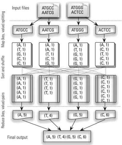
Figure 8.An illustration of the MapReduce paradigm for the symbol counting task. Mappers are applied to every element of the input sequences and emit intermediate (key, value)-pairs. Reducers are applied to all values associated with the same key. Between the map and reduce stages are some intermediate steps involving distributed sorting and grouping.

The idea of MapReduce is illustrated in Fig. 8. We initially split the original sequence into several files (e.g. two files in this case). We further split each file into several subsequences (e.g. two subsequences in this case) and ‘map’ the number of each symbol in each subsequence. The outputs of the mapper are (key, value)-pairs. We then gather together all out-put pairs of the mappers with the same key. Finally, we use a ‘reduce’ function to combine the values for each key. This gives the desired output:

#A=5,#T=4,#G=5,#C=6. The Hadoop MapReduce contains three stages, which are listed as follows.

First stage: mapping.The first stage of a MapRe-duce program is called mapping. In this stage, a list of data elements is provided to a ‘map-per’ function to be transformed into (key, value)-pairs. For example, in the above symbol-counting problem, the mapper function

sim-ply transforms each symbol into the pair (sym-bol, 1). The mapper function does not modify the input data, but simply returns a new output list.

Intermediate stages: shuffling and sorting.After the mapping stage, the program exchanges the intermediate outputs from the mapping stage to different ‘reducers’. This process is called shuf-fling. A different subset of the intermediate key space is assigned to each reduce node. These subsets (known as ‘partitions’) are the inputs to the next reducing step. Each map task may send (key, value)-pairs to any partition. All pairs with the same key are always grouped together on the same reducer regardless of which mappers they are coming from. Each reducer may process sev-eral sets of pairs with different keys. In this case, different keys on a single node are automatically sorted before they are fed into the next reducing step.

Final stage: reducing.In the final reducing stage, an instance of a user-provided code is called for each key in the partition assigned to a reducer. The inputs are a key and an iterator over all the values associated with the key. These values re-turned by the iterator could be in an undefined order. In particular, we have one output file per executed reduce task.

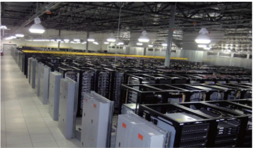
The Hadoop MapReduce builds on the HDFS and inherits all the fault-tolerance properties of HDFS. In general, Hadoop is deployed on very large scale clusters. One example is shown in Fig. 9.

Cloud computing

Cloud computing revolutionizes modern comput-ing paradigm. It allows everythcomput-ing—from hardware resources, software infrastructure to datasets—to be delivered to data analysts as a service wherever and whenever needed. Figure 10 illustrates different building components of cloud computing. The most striking feature of cloud computing is its elasticity and ability to scale up and down, which makes it suit-able for storing and processing Big Data.

IMPACT ON COMPUTATIONAL

METHODS

Big Data are massive and very high dimensional, which pose significant challenges on computing and paradigm shifts on large-scale optimization [29,94]. On the one hand, the direct application of penalized quasi-likelihood estimators on high-dimensional data requires us to solve very large scale optimization problems. Optimization with a large amount of variables is not only expensive but also

Figure 9.A typical Hadoop cluster (source: wikipedia).

suffers from slow numerical rates of convergence and instability. Such a large-scale optimization is generally regarded as a mean, not the goal of Big Data analysis. Scalable implementations of large-scale nonsmooth optimization procedures are cru-cially needed. On the other hand, the massive sample size of Big Data, which can be in the order of millions or even billions as in genomics, neuroinformatics, marketing, and online social medias, also gives rise to intensive computation on data management and queries. Parallel computing, randomized algorithms, approximate algorithms and simplified implementa-tions should be sought. Therefore, the scalability of statistical methods to both high dimensionality and large sample size should be seriously considered in the development of statistical procedures.

In this section, we explain some new progress on developing computational methods that are scalable to Big Data. To balance the statistical accuracy and computational efficiency, several penalized estima-tors such as Lasso, SCAD, and MCP have been

de-scribed in the ‘Impact on statistical thinking’ section. We will introduce scalable first-order algorithms for solving these estimators in the ‘First-order methods for nonsmooth optimization’ section. We also note that the volumes of modern datasets are exploding and it is often computationally infeasible to directly make inference based on the raw data. Accordingly, to effectively handle Big Data in both statistical and computational perspectives, dimension reduction as an important data pre-processing step is advocated and exploited in many applications [95]. We will ex-plain some effective dimension reduction methods in the ‘Dimension reduction and random projection’ section.

First-order methods for nonsmooth

optimization

In this subsection, we introduce several first-order optimization algorithms for solving the penalized quasi-likelihood estimators in (9). For most loss functions n(·), this optimization problem has

no closed-form solution. Iterative procedures are needed to solve it.

When the penalty function P_λ,γ(·) is convex (e.g. theL1-penalty), so is the objective function in (9) whenn(·) is convex. Accordingly,

sophis-ticated convex optimization algorithms can be ap-plied. The most widely used convex optimization al-gorithm is gradient descent [96], which finds a so-lution sequence converging to the optimumβ by calculating the gradient of the objective function at each point. However, calculating the gradient can be very time consuming when the dimensionality is high. Instead, the authors of [97] proposed to calculate the penalized pseudo-likelihood estimator using the pathwise coordinate descent algorithm,

which can be viewed as a special case of the gradient descent algorithm. Instead of optimizing along the direction of the full gradient, it only calculates the gradient direction along one coordinate at each time. A beautiful feature of this is that even though the whole optimization problem does not have a closed-form solution, there exist simple closed-closed-form so-lutions to all the univariate subproblems. The co-ordinate descent is computationally easy and has similar numerical convergence properties as gradi-ent descgradi-ent [98]. Alternative first-order algorithms to coordinate descent have also been proposed and widely used, resulting in iterative shrinkage-thresholding algorithms [23,24]. Prior to the coor-dinate descent algorithm, the authors of [19] pro-posed the least angle regression (LARS) algorithm to theL1-penalized least-squares problem.

When the penalty functionP_λ,γ(·) is

noncon-vex (e.g. SCAD and MCP), the objective function in (9) is no longer concave. Many algorithms have been proposed to solve this optimization problem. For example, the authors of [8] proposed a local quadratic approximation (LQA) algorithm for opti-mizing nonconcave penalized likelihood. Their idea is to approximate the penalty term piece by piece us-ing a quadratic function, which can be thought as a convex relaxation (majorization) to the noncon-cave object function. With the quadratic approxima-tion, a closed-form solution can be obtained. This idea is further improved by using a linear instead of a quadratic function to approximate the penalty term and leads to the local linear approximation (LLA) al-gorithm [27]. More specifically, given current esti-mateβ(k)=(β1(k), . . . , β

(k)

d )Tat thekth iteration

for problem (9), by Taylor’s expansion,

P_λ,γ(βj)≈Pλ,γ β(k) j +P_λ,γ β(k) j |βj| − |β(jk)| . (17) Thus, at the (k+1)th iteration, we solve

min βj ⎧ ⎨ ⎩n(β)+ d j=1 wk,j|βj| ⎫ ⎬ ⎭, (18)

wherewk,j =P_λ,γ(β(jk)). Note that problem (18)

is convex, so that a convex solver can be used. The au-thors of [58] suggested using initial valuesβ(0) =0, which corresponds to the unweightedL1 penalty. This algorithm shares a very similar idea as in [99], both of which can be regarded as implementations of the minimization of the folded-concave penal-ized quasi-likelihood [8] problem (9). If one further approximates the goodness-of-fit measuren(β) in

(18) by a quadratic function via the Taylor expan-sion, then the LARS algorithm [19] and pathwise co-ordinate descent algorithm [97] can be used.

For the more general settings where the loss func-tionn(·) may not be concave, the authors of [100]

proposed an approximate regularization path follow-ing algorithm for solvfollow-ing the optimization problem in (9). By integrating statistical analysis with com-putational algorithms, they provided explicit statis-tical and computational rates of convergence of any local solution obtained by the algorithm. Compu-tationally, the approximate regularization path fol-lowing algorithm attains a global geometric rate of convergence for calculating the full regularization path, which is fastest possible among all first-order algorithms in terms of iteration complexity. Statis-tically, they show that any local solution obtained by the algorithm attains the oracle properties with the optimal rates of convergence. The idea on study-ing statistical properties based on computational al-gorithms, which combine both computational and statistical analysis, represents an interesting future direction for Big Data. We also refer to [101] and [102] for research studies in this direction.

Dimension reduction and random

projection

We introduce several dimension (data) reduction procedures in this section. Why do we need di-mension reduction? Let us consider a dataset repre-sented as ann×dreal-value matrixD, which en-codes information aboutnobservations ofd vari-ables. In the Big Data era, it is in general compu-tationally intractable to directly make inference on the raw data matrix. Therefore, an important data-preprocessing procedure is to conduct dimension re-duction which finds a compressed representation of

Dthat is of lower dimensions but preserves as much information inDas possible.

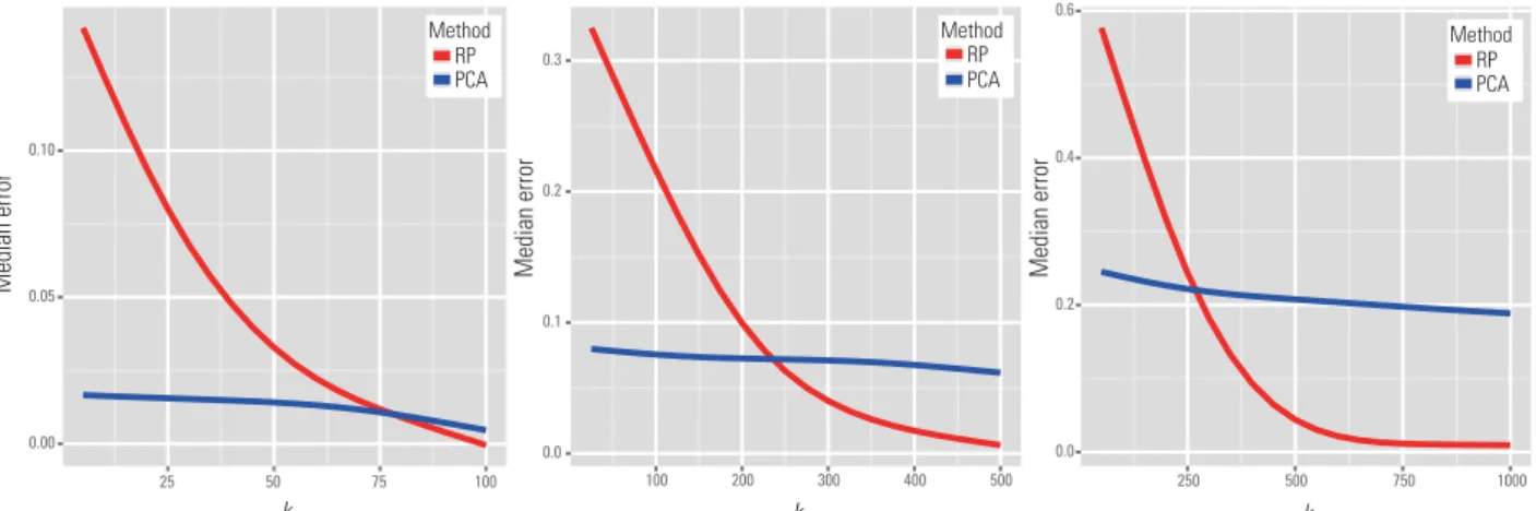
Principal component analysis (PCA) is the most well-known dimension reduction method. It aims at projecting the data onto a low-dimensional orthog-onal subspace that captures as much of the data vari-ation as possible. Empirically, it calculates the lead-ing eigenvectors of the sample covariance matrix to form a subspaceUk∈Rd×k. We then project then ×ddata matrixDto this linear subspace to obtain ann×kdata matrixDUk. This procedure is

opti-mal among all the linear projection methods in min-imizing the squared error introduced by the projec-tion. However, conducting the eigenspace decom-position on the sample covariance matrix is compu-tational challenging when bothnanddare large. The computational complexity of PCA isO(d2_n+d3₎ [103], which is infeasible for very large datasets.