S. Descombes, B. Dussoubs, S. Faure, L. Gouarin, V. Louvet, M. Massot, V. Miele, Editors
COMPASS : A TOOL FOR DISTRIBUTED PARALLEL FINITE VOLUME
DISCRETIZATIONS ON GENERAL UNSTRUCTURED POLYHEDRAL MESHES
E. Dalissier
1, C. Guichard
2, P. Hav´
e
3, R. Masson
4et C. Yang
5R´esum´e. L’objectif du projet ComPASS est de d´evelopper un code parall`ele de simulation des ´
ecoulements polyphasiques en milieux poreux adapt´e aux maillages non structur´es poly´edriques (en un sens g´en´eralis´e avec des faces potentiellement non planes) et `a une grande classe de sch´emas de discr´etisation volume fini utilisant des degr´es de libert´e vari´es comme par exemple des inconnues centr´ees aux mailles, des inconnues de face ou encore des inconnues aux nœuds. Les principales ap-plications vis´ees sont la simulation du stockage g´eologique du CO2, la mod´elisation des stockages de d´echets radioactifs ou encore la simulation des r´eservoirs p´etroliers et gaziers.
L’´ecole d’´et´e du CEMRACS 2012 consacr´ee au calcul haute performance a constitu´e un cadre id´eal pour d´emarrer ce projet collaboratif. Cet article d´ecrit les d´eveloppements r´ealis´es durant les 4 semaines du projet qui ont mis l’accent sur les fonctionnalit´es de base du code ComPASS tels que les structures du maillage distribu´e, la synchronisation des degr´es de libert´e, et la connexion `a des biblioth`eques scientifiques comme le partitionneur METIS, l’outil de visualisation PARAVIEW ou encore la biblioth`eque de solveurs lin´eaires parall`eles PETSc. L’efficacit´e parall`ele de cette premi`ere version du code ComPASS a ´et´e valid´ee sur l’exemple simple d’un probl`eme parabolique discr´etis´e en temps par un sch´ema d’Euler implicite et en espace par le sch´ema volume fini Vertex Approximate Gradient utilisant `a la fois des inconnues aux mailles et aux nœuds.
Abstract. The objective of the ComPASS project is to develop a parallel multiphase Darcy flow simulator adapted to general unstructured polyhedral meshes (in a general sense with possibly non planar faces) and to the parallelization of advanced finite volume discretizations with various choices of the degrees of freedom such as cell centres, vertices, or face centres. The main targeted applications are the simulation of CO2 geological storage, nuclear waste repository and reservoir simulations.
The CEMRACS 2012 summer school devoted to high performance computing has been an ideal framework to start this collaborative project. This paper describes what has been achieved during the four weeks of the CEMRACS project which has been focusing on the implementation of basic features of the code such as the distributed unstructured polyhedral mesh, the synchronization of the degrees of freedom, and the connection to scientific libraries including the partitioner METIS, the visualization tool PARAVIEW, and the parallel linear solver library PETSc. The parallel efficiency of this first version of the ComPASS code has been validated on a toy parabolic problem using the Vertex Approximate Gradient finite volume spatial discretization with both cell and vertex degrees of freedom, combined with an Euler implicit time integration.
1 LJK UMR 5224 Universit´e de Grenoble,[email protected]
2LJAD UMR 7351 Universit´e de Nice Sophia Antipolis & team COFFEE INRIA Sophia Antipolis Mediterran´ee,[email protected] 3 IFP Energies nouvelles, Rueil-Malmaison,
4LJAD UMR 7351 Universit´e de Nice Sophia Antipolis & team COFFEE INRIA Sophia Antipolis Mediterran´ee,[email protected] 5 ICJ UMR 5208 Universit´e de Lyon 1,[email protected], this author is partially supported by European Research
Council ERC starting Grant 2009, project 239983-NuSiKiMo.
c
EDP Sciences, SMAI 2013
Introduction
ComPASS, standing for Computing Parallel Architecture to Speed up Simulations, is a project focusing on the solution of time-evolution problems on general polyhedral meshes using Finite Volume (denoted FV in the following) discretizations which has been the subject of active researches over the last decades. The long-term ambition of this project is to develop a parallel prototype code in order to implement and compare on relevant problems a large class of promising FV schemes with degrees of freedom (d.o.f.) typically located at cells, faces or vertices as exhibited in the recent 3D benchmark for diffusion problems [16]. The targeted applications are those of the INRIA project team COFFEE (COmplex Flows For Energy and Environment), such as the modelization of multiphase flows in porous media applied to oil and gas recovery in petroleum reservoirs, oil exploration in sedimentary basins, the geological storage of CO2 in saline aquifers or the disposal of high level radioactive waste.
These applications imply the simulation of multiphase Darcy flows in heterogeneous anistropic porous media, strongly coupling the mass conservation laws with the local hydrodynamical and thermodynamical closure laws and involving a large range of time and space scales. The time integration schemes are usually fully implicit in order to allow for large time steps. The spatial discretization is typically a FV scheme with an approximation of the Darcy fluxes splitting their elliptic part (see−Λ(x)∇Pαin (1) below) and their hyperbolic part (mobility terms mαi(x, U) in (1) below). The discretization of the elliptic part represents the main difficulty on which we will be focusing since it must be adapted to complex meshes, and to the anisotropy and heterogeneity of the porous media. Most recent FV schemes use various d.o.f. such as cell, face, or vertex unknowns for the approximation of these fluxes. They are compact in the sense that the stencil of the scheme is limited to un-knowns located at the neighbouring cells of a given d.o.f (in the sense that they share a vertex). The hyperbolic part of the fluxes is usually only dealt with a first order upwind approximation to allow for fully implicit time integration, and hence it does not break the compacity of the scheme in the above sense. These FV implicit discretizations lead to solve at each time step and at each Newton type iteration, ill conditioned large sparse linear systems using preconditioned Krylov methods.
The authors have already developed several non parallel codes implementing multiphase Darcy flow models with various FV schemes. Given the high memory requirements of these type of applications, these codes were limited basically to 2D or coarse 3D meshes. In order to overcome these limitations, both in terms of memory and CPU time, we have decided to start the implementation of a new code using a parallel distributed approach. A first crucial step toward this objective is to develop a tool adapted to general polyhedral meshes, which should be able to partition the mesh and to distribute it on a given number of processes, to compute FV schemes using various d.o.f. such as cell, face and vertex unknowns, to assemble and solve in parallel non linear and linear systems within a time loop, and to visualize the solutions at given time steps. In order to make this project tractable in a small amount of time, we decided to focus on the following specifications:
• general meshes including polyhedral cells with an arbitrary number of faces and possibly non planar faces,
• various and open request connectivities for cells, faces, and vertices, and one full layer of ghost cells (including all its cell, face and vertex d.o.f.) in order to easily compute and assemble locally on each processor a large class of compact FV discretizations,
• in order to simplify the first implementation, limit in a first step the size of the problem up to say 107
cells on a maximum number of one thousand processes.
However, it was not clear that these libraries were easy to adapt in order to deal with general polyhedral meshes, and our team did not include advanced users of these libraries. Alternatively, in order to have an easy full control on the core of the code (mesh format, connectivity and distribution, FV schemes, physics, assembly of the non-linear and linear systems) we have decided to develop it from scratch and to rely on existing up to date scientific computing libraries only for specific tasks such as the partitioner, the linear solver and the visualization tools. Among well known programming languages for High Performance Computing (HPC), Fortran 90 combined with MPI has been chosen for our implementation rather than an object oriented language like C++ mainly because our team is already experienced with Fortran 90 and not with C++. The research session of the CEMRACS 2012 summer school, devoted to HPC, and joining at the CIRM around 100 researchers during 5 weeks, has been clearly a perfect framework to start the development of the ComPASS project.
1.
Models and discretization
As stated in the introduction, the final goal of the ComPASS project is to simulate complex flows in geo-sciences such as compositional multiphase flows in porous media used in many applications. For example, in oil reservoir modelling, the compositional triphase Darcy flow simulator is a key tool to predict and optimize the production of a reservoir. In sedimentary basin modelling, such models are used to simulate the migration of the oil and gas phases in a basin saturated with water at geological space and time scales. The objectives are to predict the location of the potential reservoirs as well as the quality and quantity of oil trapped therein. In CO2 geological storage, compositional multiphase Darcy flow models are used to optimize the injection of CO2 and to assess the long term integrity of the storage. The numerical simulation of such models is a challenging task, which has been the subject of a lot of works over a long period of time, see the reference books [8] and [21]. Let us briefly sketch the framework of these models.
We recall here the basis of the Coats’ formulation [10] for compositional multiphase Darcy flow models. Let
Pdenote the set of possible phasesα∈P, andCthe set of componentsi∈C. Each phaseα∈Pis described by its non empty subset of componentsCα⊂Cand is characterized by its thermodynamical and hydrodynamical properties depending on its pressurePα, its molar compositionCα= (Cα
i )i∈Cα, and on the volume fractions or
saturations denoted byS = (Sα)
α∈P. The phases can appear or disappear due to thermodynamical equilibrium,
which leads to the introduction of the new variableQ⊂P representing the number of present phases at each point of the space time domain. The set of unknowns of the system in the Coat’s formulation is defined by
U = (Pα, Sα, α∈P, Cα, α∈Q) and the flow is governed by the following conservation equations,
φ(x)∂tni(U) + X
α∈Q
div (−mαi(x, U) Λ(x)∇P
α) = 0, for alli
∈C, (1)
where ni denote the number of moles of the component i ∈ C per unit volume, mαi is roughly speaking the mobility of the component iin the phase α, φ(x) and Λ(x) are respectively the porosity and the permeability tensor and both are functions of the position x in space. The system is closed by the hydrodynamical and thermodynamical laws as well as the volume balance equationP
α∈PS
α= 1. We refer to [15] and the references
therein for a more detailed discussion about this formulation.
There are two main difficulties to solve such models coupling parabolic/elliptic and hyperbolic/degenerate parabolic unknowns. First, degeneracies appear in the set of equations (1) typically at the end points of the hydrodynamical laws, and at phase transitions. Second, the heterogeneous and anisotropic nature of the media leads to possibly strong jumps of the permeability tensor Λ(x), of the porosityφ(x), and also of the mobilities
mαi(x, U) and of the capillary pressuresPc,α,β(x, S) =Pα−Pβ.
meshes and to anisotropic heterogeneous media has been the object of intensive research in the last two decades and has lead to numerous schemes using various d.o.f. as exhibited in the recent 3D benchmark for diffusion problem [16]. Nevertheless, finding the ’best’ FV scheme is still a problem dependent issue and the main objective of the ComPASS project is to build an appropriate tool to test promising schemes on problems with realistic physics, mesh size, and time scales, using parallel distributed computations.
1.1.
A 3D mesh format for unstructured general grids
In geological applications, in order to capture the geometry and the main heterogeneities of the media, the grid generation is constrained to match the main structural features of the reservoir or basin geometry defined by the geological sedimentary layers possibly cut by a network of faults.
For that purpose, the most commonly used mesh format in reservoir simulation is still the so called Corner Point Geometry (CPG) which is a globally structured hexahedral grid, locally unstructured due to erosion leading to degenerate hexahedra (collapse of edges, or of entire faces), and locally non-matching due to faults as illustrated in Figure 1. In addition, non-conforming Local Grid Refinement (LGR) can be used in nearwell regions.
Figure 1. Examples of general cells due to geological erosion (left part) or faults (the last at the right).
Although CPG grids are widely used for full field reservoir simulations, they are not adapted to modelize complex fault networks such as Y-shaped faults at basin scales, nor to discretize complex geometries at finer scales such as in the neighbourhood of complex wells or fracture networks. This justifies the growing interest to use unstructured meshes for such applications. For instance, let us consider a 3D nearwell mesh exhibited in Figure 2. The first step of the discretization is to create a radial mesh that is exponentially refined down to the well boundary to take into account the singular behaviour of the pressure close to the well. Then, this radial grid is matched to the reservoir grid using tetrahedra as well as pyramids at the interface, as can be seen in Figure 2(b). This transition zone enables to couple the nearwell simulation to a global reservoir simulation.
(a) exponentially re-fined radial mesh
(b) hybrid mesh with hexahedra, tetrahedra and pyramids
Figure 2. Space discretization of a deviated well.
format with a description of the cells by their set of faces and of the faces by their set of vertices given in cyclic order. It is assumed that the possible non-conformities have been solved by computing the co-refinement of the surfaces on both sides of the non-conformities generating a conforming mesh with general polyhedral cells. Our format is very close to the one used for the 3D benchmark [16] without the description of the set of edges which is expensive in terms of memory requirement and usually not used in practice for most FV schemes. For the sake of simplicity, it will be assumed in the following that the edge data structure is not used. It could always be computed and added if required by the discretization scheme. Let us also specify that the rock properties such as the permeability tensor and the porosity will be defined as usual as cellwise constant.
D´efinition 1.1 (Admissible space discretization). Let Ω be an open bounded subset of R3 and∂Ω = Ω\Ω its boundary. An admissible space discretization of Ω is defined by assuming that a primary polyhedral meshMis given where each element (“commonly named cell”)K∈ M is strictly star-shaped with respect to some point
xK, called the centre ofK. We then denote byFK the set of interfaces of non zero two dimensional measure among the inner interfacesK∩L,L∈ M, and the boundary interfaceK∩∂Ω possibly split in several boundary faces. Eachσ∈ FK (“face ofK”) is assumed to be the union of triangles τ∈ Sσ. We denote byVσ the set of all the vertices ofσ, located at the boundary ofσ(“vertices ofσ”), and byV0
σthe set of all the internal vertices ofσ. Therefore, the 3 vertices of anyτ ∈ Sσ are elements ofVσ0∪ Vσ. Let us denote by
F= [ K∈M
FK
the set of faces, and by
V = [ σ∈F
Vσ,
the set of vertices of the meshM.
In practice, it will be assumed that the setV0
σ reduces to the isobarycentre of the set of verticesVσ. Hence, the mesh format reduces to a numbering of the cellsM, of the facesFand of the verticesV, to the coordinates of the vertices, to the definition of the setsFK for all cellsK∈ M, and of the setsVσ in cyclic order for each face σ∈ F. In addition, the set of neighbouring cellsMσ is given for each faceσ∈ F. It is well known that, for a conforming mesh, the setMσ contains either two cells for an inner face and one cell for a boundary face.
1.2.
Example of the VAG scheme on a parabolic problem
In the short term of the CEMRACS, it has been decided to implement the following simple linear parabolic equation,
∂tu(x, t)− 4u(x, t) =f(x, t), (2)
in the space-time domain Ω×(0, T), with the initial conditionu(x,0) =uini(x), for a.e. x∈Ω,and an
homo-geneous Dirichlet boundary condition, under the following assumptions:
• Ω is an open bounded connected polyhedral subset of R3, andT >0, • f ∈L2(Ω×(0, T)) anduini∈L2(Ω).
The implementation of this simple model already includes most of the features required for more complex models such as the compositional Darcy flow model (1): a time loop for time integration, the discretization of a second order elliptic operator that will be implemented using FV fluxes, and the solution of a linear system at each time step.
face unknowns in addition to the cell unknowns. The DDFV (Discrete Duality Finite Volume) scheme [7] uses both cell and vertex unknowns. For our test case, we have chosen to implement the VAG (Vertex Approximate Gradient) scheme, also using both cell and vertex d.o.f. It has been introduced in [14] in the framework of the gradient schemes. We will briefly describe the main characteristics of this scheme and we refer to [15] for its application to multiphase Darcy flows.
1.2.1. Gradient schemes for a parabolic problem
The gradient schemes were recently introduced in order to obtain a uniform framework for the definition and the convergence analysis of a large family of schemes including conforming discretizations (such as finite element methods) and non conforming discretizations (such as mixed finite element and finite volume methods). The gradient schemes framework has already been applied to several problems, we mention especially here the case of the Stefan problem [12] since it includes our simple model (2) as a particular case.
Gradient schemes are based on the weak primal formulation of the model which in the case of the parabolic equation (2) leads to the following variational formulation: findu∈L2(0, T;H1
0(Ω)) such that
RT
0
R
Ω(−u(x, t)∂tϕ(x, t) +∇u(x, t)· ∇ϕ(x, t)) dxdt−
R
Ωuini(x)ϕ(x,0)dx=
RT
0
R
Ωf(x, t)ϕ(x, t)dxdt, (3)
for all ϕ∈Cc∞(Ω×[0, T[). The spirit of the gradient schemes is to replace the continuous operators by their discrete versions leading to the following definition of a space gradient discretization.
D´efinition 1.2 (Space gradient discretization). A space gradient discretization of the problem (3) is defined byD= (XD,0,ΠD,∇D) where,
(1) the set of d.o.f. XD,0 is a finite dimensional vector space on R suited to the Dirichlet homogeneous boundary condition,
(2) the linear mapping ΠD : XD,0→L2(Ω) is the reconstruction of the approximate function,
(3) the linear mapping∇D : XD,0 →L2(Ω)3 is the discrete gradient operator. It must be chosen such
that k · kD :=k∇D· kL2(Ω)3 is a norm onXD,0.
The time interval (0, T) is discretized using, for the sake of simplicity, a constant time step denoted byδtand defined byδt=t(n+1)−t(n) withn= 0, . . . , N such thatt(0)= 0< t(1). . . < t(N)=T.
The problem (3) is then approximated by a space-time gradient discretization using the following Euler implicit time integration scheme. Givenu(0)∈X
D,0with ΠDu(0)an approximation ofuini, the discrete solutions
u(n)∈X
D,0 satisfy
R
Ω
ΠD
u(n+1)−u(n)
δt (x)ΠDw(x) +∇Du
(n+1)(x)· ∇
Dw(x)
dx= 1
δt Rt(n+1)
t(n) R
Ωf(x, t)ΠDw(x)dxdt,
∀w∈XD,0, ∀n= 0, . . . , N−1.
(4)
1.2.2. Definition the VAG scheme
Following the Definition 1.1 of the space discretization of Ω, we also defineVK as the set of all elements of
V which are vertices ofK. For anyK ∈ M,σ∈ FK,τ ∈ Sσ, we denote by SK,τ the tetrahedron with vertex
xK and basisτ as illustrated in the Figure 3.
Let us then define the gradient scheme space and operators of Definition 1.2 for the VAG scheme.
• We define XD,0 as the space of all vectors u = ( (uK)K∈M , (uv)v∈V ), uK ∈ R, uv ∈ R such that uv= 0 for allv∈ V ∩∂Ω.
v∈ V0 σ
xK
Figure 3. Tetrahedral submesh.
• The mapping ∇D is defined, for any u ∈ XD,0, by ∇Du = ∇ΠbDu, where ΠbDu is the continuous
reconstruction which is affine in all SK,τ, for allK ∈ M, σ∈ FK and τ ∈ Sσ, with the values uK at
xK, uv at any vertex vof τ which belongs toVσ, and Px∈Vσα x
vux at any vertexv ofτ which belongs toV0
σ, where the coefficientsαxv, x∈ Vσ are the barycentric coordinates ofv.
Using the above definition of the VAG scheme, and precisely thanks to the result that for all x ∈ K, for
K∈ M, the discrete gradient∇Du(x) is expressed as a linear combination of (uK−uv)v∈VK, the Problem (4) can be rewritten as follows,
P K∈M
R K
u(Kn+1)−u(Kn)
δt wK+
P K∈M
P
v∈VKFK,v(u n+1)(w
K−wv) = PK∈M
1
δt Rt(n+1)
t(n) R
Kf(x, t)wKdxdt,
∀w∈XD,0, ∀n= 0, . . . , N−1,
(5) whereFK,v(un+1) is interpreted as the flux from a cellK∈ Mto one of its verticesv∈ VK and is defined by,
FK,v(un+1) = P v0∈V
KT v,v0
K (u
(n+1)
K −u
(n+1)
v0 ). (6)
Remarque 1.3. Thanks to the definition of the above fluxes, the VAG scheme can be seen as a FV method. For this, we need to define some disjoint arbitrary control volumes VK,v ⊂ Sv∈τSK,τ for all K ∈ M and
v ∈ VK. It is important to notice that it is not in general necessary to provide a more precise geometric description ofVK,v than its volume. The mapping ΠD is then defined for anyu∈XD,0 by ΠDu(x) =uK, for a.e. x ∈ K\S
v∈VKVK,v, and by ΠDu(x) = uv for a.e. x ∈ VK,v. Finally, related to the Definition (6) of the fluxes, the VAG scheme can be seen as a MPFA FV method for multiphase Darcy flow models in the set of control volumes defined as the union of the cells and of the vertices. We refer to [15] for a more detailed discussion.
1.2.3. Implementation and discussion
Finally, setting in (5), on the one hand wv = 1 with all other values equal to zero, and, on the other hand
u(0)∈X
D,0, findu(n+1)∈XD,0 at each time stepn≥0 such that
X
K∈Mv X
v0∈V
K
−TKv,v0(u(Kn+1)−uv(n0+1)) = 0 ∀v∈ V\∂Ω, . (7a)
|K| δt (u
(n+1)
K −u
(n)
K ) + X
v∈VK X
v0∈V
K
TKv,v0(u(Kn+1)−uv(n0+1)) =|K|f(xK) ∀K∈ M, (7b)
where|K|is the volume of the cellK andMv is the set of cells sharing the vertexv, defined by
Mv={K∈ M |v∈ VK}.
The advantage of this scheme is that it allows to eliminate without any fill-in all the cell unknowns (uK)K∈Mby
using the equation (7b). The system reduces to the Schur complement on the vertex unknowns (uv)v∈V leading
to a compact vertex centred scheme. Its stencil involves only the neighbouring vertices of a given vertex, with a typical 27 points stencil for 3D topologically Cartesian meshes. Let us also point out that the VAG scheme applies to general meshes with possibly non planar faces. In addition, the VAG scheme is consistent and unconditionally coercive and has exhibited a good compromise between accuracy, robustness and CPU time in the recent FVCA6 3D benchmark [16].
In particular, the VAG fluxes can be used for the discretization of multiphase Darcy flows leading to a very efficient scheme on tetrahedral meshes or on hybrid meshes combining typically tetrahedra, hexahedra and pyramids. For such problems on tetrahedral meshes, the VAG scheme is say 15 times more efficient in comparison with cell centred discretizations such as the MPFA O-scheme. This result can be explained by the ratio of around 5 between the numbers of cells and the number of vertices, and by the very large stencil of the MPFA O-scheme on such meshes (about 3 times larger than the stencil of the VAG scheme). In addition, the usual difficulties of vertex centred approaches to deal with multiphase Darcy flows in heterogeneous media can be solved thanks to the fact that the cell unknown is kept in the discretization and thanks to the flexibility provided by the VAG scheme in the choices of the volumesVK,v(see [15] for more details).
2.
ComPASS parallel distributed processing
In this section, assuming that a mesh satisfying Definition 1.1 is given, the main steps of the algorithm for the parallel distributed solution of equation (7) is detailed (see also Figure 4). It will be assumed that the topology of the mesh does not change during the time evolution. Consequently, the partitioning and the distribution of the mesh on the set of processesP will be done in a preprocessing step once and for all. Also in order to define the overlaps between processes (ghost cells, faces or vertices), the FV schemes are assumed to be compact in the sense that their stencil involves only d.o.f. located at the neighbouring cells of a given item. This remark leads to our definition of the overlap as one layer of cells.
ComPASS fits into the SPMD (Single Program, Multiple Data) paradigm. To simplify the implementation, it is assumed that a master process reads and stores the mesh, computes the partitioning, and distributes the local meshes to each process. After distribution of the mesh by the master process, all the computation are done in parallel, and synchronisations of the d.o.f. at the ghost items can be performed in order to match the overlapping d.o.f. between the processes. Following our example of equation (7), we will describe the parallel computation of the FV scheme as well as the assembling and the solution of the linear system at each time step using the PETSc [4] library. Thanks to our general definition of the overlap, the assembling step will be done locally on each process without communication.
2.1.
Distributed mesh
•mesh reader
•mesh distribution
•messages ordering
•memory preallocation
•VAG scheme computation
•matrix and RHS assembling
•linear system resolution
•synchronisation of node values
•Schur complement for cell values
•postprocessing
Initialization Time loop
Figure 4. Main steps of the algorithm for the parallel distributed solution of equation (7).
Procp0
Ip0
Ip0/ Ip0
Procp1
Ip1
Ip1/ Ip1
⋯
Procpn−1
Ipn−1
Ipn−1/ Ipn−1
Figure 5. The overlapping decompositions of the sets of cells, vertices and faces. I =
M,V, orF;n= card(P).
vertices, we have chosen to partition the set of cells
M= [ p∈P
Mp. (8)
The overlapping decomposition of the set of cells
Mp, p∈ P,
is chosen in such a way that all compact finite volume schemes can be assembled locally on each processor. Hence Mpis defined as the set of all cells sharing a vertex with Mp.
The overlapping decompositions of the sets of vertices and faces follow from this definition
Vp= [
K∈Mp
VK, p∈ P,
for the set of verticesV, and
Fp= [
K∈Mp
FK, p∈ P,
for the set of facesF. These overlapping decompositions are sketched in Figure 5.
All these decompositions are computed on the master process from the initial mesh. The partitioning of the set of cells Mis computed by the subroutineMETIS PartGraphRecursive of the Metis library [3] which uses a multi-constraint multilevel recursive bisection algorithm to minimize the number of edge cuts. It is provided with the number of processes card(P), and with the sets MK, forK∈ M of cells connected toK by a vertex defined by
MK = [
v∈VK
Mv.
The next step is to choose the partitioning of the remaining sets of items, i.e. the set of verticesV and the set of facesF. Let us start first with the vertices, the methodology is similar for the faces. The partitioning of the set of vertices is obtained by a rule of belonging of a given vertex to a processp∈ P, chosen to ensure a well balanced partitioning. To be more specific, let us denote by #M K the unique global index of a cell K∈ M.
We have the following definition.
D´efinition 2.1 (Partitioning of the set of vertices). A vertexv∈ V belongs to the same processp∈ P as the process of the cell with the smallest global index #M K among the set Mv of cells sharingv. Following this rule, we obtain the partitioningV=S
p∈PVp with
Vp={v∈ V |K(v)∈ Mp}, p∈ P,
where, for allv∈ V,K(v) = argminL∈Mv{#M L}.
Similarly the partitioning of the set of facesF is given by the following definition.
D´efinition 2.2 (Partitioning of the set of faces). A face σ ∈ F belongs to the same process p ∈ P as the process of the cell with the smallest global index #M K among the setMσ of cells sharingσ. Following this rule, we obtain the partitioningF=S
p∈PFp with
Fp={σ∈ F | K(σ)∈ Mp}, p∈ P,
where, for allσ∈ F,K(σ) = argminL∈M
σ{#M L}.
Let us emphasize that one clearly has from the above definitions that
Vp⊂ [
K∈Mp
VK andFp⊂ [
K∈Mp
FK.
It results, thanks to our choice of the overlaps, that the computation of the FV schemes will always be done locally on each process without communication, for all compact schemes requiring only one layer of neighbouring cells.
2.2.
Communication and synchronization between processes
A basic ingredient for the parallelization of the solution algorithms is the synchronization of the d.o.f defined at the ghost items Ip\ Ip, for all p ∈ P, and for I = M,V or F. This synchronization is achieved using MPI (Message Passing Interface, see [17, 18] for basic references) Send and Receive communications between processes. To that end, the following subsets ofP are computed in a preprocessing step once and for all: first the subsets of processes from whichpmust receive ghost items
PIp,←={q∈ P\{p} | Ip∩ Iq6=
∅}, I =M,F,V, p∈ P, (9)
and second, the subsets of processes to whichpneeds to send ghost items
PIp,→={q∈ P\{p} | Ip∩ Iq6=
∅}, I =M,F,V, p∈ P. (10)
For each mesh itemI=M,V,F, we also store once and for all, for each processp∈ P, the partitioning
Ip\ Ip= [ q∈PIp,←
Ip Procp
Ip∩ Iq0
Procq0
⋯
Ip∩ IqiProcqi
⋯
Ip∩ Iq(n→p,I−1)
Procq(n→
p,I−1)
(a)
mi
Ip /Ip Procp
Iq0∩ Ip
Procq0
⋯
Iqj∩ IpProcqj
⋯
Iq(n←p,I−1)∩ I p
Procq(n←
p,I−1)
(b)
mj
Figure 6. Communication of processor p ∈ P with other processors. (a) the processor p
sends message mi = (Send, p, qi) to the processor qi ∈ PIp,→, i= 0, . . . , n→p,I−1, with n→p,I =
card(PIp,→); (b) the processor p receives message mj = (Receive, p, qj) from the processor
qj∈ PIp,←, j= 0, . . . , np,←I−1, withn←p,I = card(P
p,← I ).
of the ghost items ofp(see Figure 6 (b)), and the partitioning
Ip∩
[
q∈P,q6=p
Iq
=
[
q∈Pp,→ I
Ip∩ Iq, (12)
of the own items ofpbelonging to the ghost items ofq6=p,q∈ P (see Figure 6 (a)).
These partitionings define the set of Send and Receive MPI messages that need to be sent and received to synchronize a given vectorwp, p∈ P withwp∈VIp
, where V is a given vector space of d.o.f (typicallyRn for n a given number of unknowns per item). The synchronization provides the values of the vector at the ghost items on each process p∈ P defining the overlapping vectorwp, p∈ Pwithwp∈VIp.
For each mesh item I = M,V,F, the set of all Send and Receive messages for a given process p ∈ P is denoted by
MpI={(Receive, p, q), q∈ PIp,←} ∪ {(Send, p, q), q∈ PIp,→}, (13) where, for the message m= (Send, p, q), the processpsends to q∈ PIp,→ the values of wp at the set of items
Ip∩ Iq, and for the messagem= (Receive, p, q), the processpreceives inwp from q∈ Pp,←
I the values ofwq
at the set of itemsIq∩ Ip.
D´efinition 2.3 (Complementary message). For a given mesh item I = M,V,F, and a given messagem = (mtype, p, q), we denote bym−1 its complementary message which is defined by m−1 = (mtype−1, q, p) where
Send−1= Receive, and symmetrically Receive−1= Send.
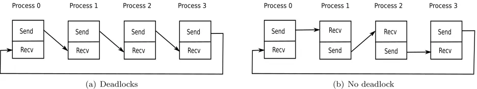
We have chosen to write the synchronization algorithm in a way that the execution will be deterministic and reproducible. This choice requires to use blocking point-to-point communications and an ordering of the messages to avoid possible deadlocks. This strategy has already proven its efficiency in the Arcane Framework [19] achieving a good scalability of the synchronization algorithm on more than 10000 processes.
Following [20, Subsection 2.1], there are two situations of deadlock that can occur when using blocking point-to-point MPI communications:
(d1) for a given message, its complementary message does not exist,
The first case (d1) is avoided thanks our definition of the sets (9)-(10)-(13). Indeed, considering a mesh item
Iand a processp∈ P, then, for a given messagem∈MpI, there clearly exists a unique processq∈ PIp,←SPp,→
I
such thatm−1∈Mq
I.
A Send-Receive cycle (d2) arises when two (or more) processes are all waiting for their complementary messages. Let us illustrate this case in the example exhibited on Figure 7 taken from [20, Subsection 2.1]. In this example P = {pi, i = 0,3} and the set of messages (13) of each process is defined by MpIi =
{(Send, pi, pi+1) , (Receive, pi, pi+1)} fori∈J0,3K, p4 =p0, withI a fixed mesh item. On the subfigure 7(a),
deadlocks occur since all processes are sending their send message first. The reordering of the sets (MpiI)i=0,3
proposed on the subfigure 7(b) allows to avoid such occurrence.
Send
Recv Send
Recv
Send
Recv
Send
Recv
Process 0 Process 1 Process 2 Process 3
(a) Deadlocks
Send
Recv Send
Recv Send
Recv
Send Recv
Process 0 Process 1 Process 2 Process 3
(b) No deadlock
Figure 7. Example of communications between four processes.
We have to define a proper ordering of the set of messages MpI in order to avoid deadlocks of type (d2). Roughly speaking our ordering rule will prescribe that:
(a) each process p performs its sendings and receptions in ascending order of the process ranks q ∈ PIp,←S
PIp,→,
(b) when two processespandqcommunicate, the one with lowest rank must sends its message first. To be more specific, let us denote by #pthe rank of a processp∈ P. Given two messagesmi= (mtypei, p, qi),
i= 1,2,m16=m2 belonging toMpI, they are ordered according to the rule in the following Table 1.
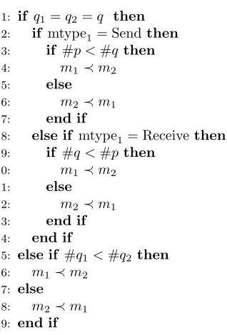
Th´eor`eme 2.4(Synchronisation without a deadlock situation (d2)). For a given mesh itemI=M,V,F, the execution of the messages in the ordering defined in the Table 1 applied to each set MpI, for allp∈ P, leads to a synchronisation without a deadlock occurrence in the sense of definition (d2).
Proof. Let P = {pi}i=1,n the set of processes, with card(P) = n > 2, and # pi = i for all i = 1,· · ·, n. We assume, for the sake of simplicity, that all processes communicate, possibly with empty messages. This assumption simplifies the writing of the proof and corresponds in practice to a worst case assumption. Indeed, an empty message implies that its complementary message is also empty, which means in practice that no communication arises between both processes. The proof will be shown to hold even if a communication is considered in such a case.
The proof is done by induction over the number of processesn, and for a given mesh itemI. Thus, let us first prove the result forn= 2. The ordering of the two sets of messages,Mp1
I andM
p2
I is done
according to the point (b) of our ordering rule (corresponding to the lines (1−14) of the algorithm described in the Table 1). It results that the ordered sets of messages are Mp1
I = [ (Send, p1, p2) ≺ (Receive, p1, p2) ]
and Mp2
I = [ (Receive, p2, p1) ≺ (Send, p2, p1) ]. It is clear that at the first execution step, the process p1
executes the message (Send, p1, p2) and the process p2 executes the complementary message (Receive, p2, p1).
Then, at the second step the process p2 executes the message (Send, p2, p1) and the process p1 executes the
complementary message (Receive, p1, p2) which shows that the communications are achieved without deadlock.
Let us now assume that the result is satisfied fornprocesses, and check that it is still true forn+ 1 processes. We denote byMf
pi
I, for i= 1,· · ·, n, the ordered sets of messages between the firstn processes which are, by
assumption, well ordered to avoid a deadlock. The sets Mpi
I, for a giveni ∈J1, nK, are the union of fM
pi
1: if q1=q2=q then
2: if mtype1= Sendthen
3: if #p <#qthen
4: m1≺m2
5: else
6: m2≺m1
7: end if
8: else if mtype1= Receivethen 9: if #q <#pthen
10: m1≺m2
11: else 12: m2≺m1
13: end if 14: end if
15: else if #q1<#q2then
16: m1≺m2
17: else 18: m2≺m1
19: end if
Table 1. Ordering of two messages m1 6=m2 ∈ MIp with mi = (mtypei, p, qi), i = 1,2 and wheremi≺mj means that the messagemi has to be executed beforemj fori6=j.
of the messages (Send and Receive) between the processes pi, i∈J1, nK andpn+1. Since the processpn+1 has
the highest rank, applying point (a) of our ordering rule (corresponding to the lines (15−19) of the algorithm presented in the Table 1), each set of messages Mpi
I, fori= 1,· · ·, n, is ordered starting with the ordered set
f Mpi
I. Then, using the point (b) of our ordering rule, we obtain the ordering,
MpiI = [Mf pi
I ≺ (Send, pi, pn+1) ≺ (Receive, pi, pn+1) ], ∀i∈J1, nK.
Similar arguments lead to the following ordering of the set of messages of the processpn+1,
Mpn+1
I = [ (Receive, pn+1, p1) ≺ (Send, pn+1, p1) ≺ · · · ≺ (Receive, pn+1, pn) ≺ (Send, pn+1, pn) ].
It results from our induction assumption that the messages (fM pi
I)i=1,nwill be executed first without deadlock. Next, from the above ordering of the messages, fori= 1,· · ·, nin this order:
• the processpi executes the message (Send, pi, pn+1),
• the processpn+1 executes the complementary message (Receive, pn+1, pi),
• the processpi executes the message (Receive, pi, pn+1),
• the processpn+1 executes the complementary message (Send, pn+1, pi).
We conclude that all the communications are achieved without deadlock.
2.3.
Computation of the Finite Volume scheme
From our choice of the overlaps, the computation of the FV scheme can always be done locally on each process without communications, for all schemes requiring only one layer of neighbouring cells.
transmissivities can be computed only once in the simulation, before the time-loop. Similarly, the cell volumes
|K|and the cell centresxK are also computed locally for allK∈ Mp and for each processp∈ P.
2.4.
Assembly of the linear system and linear solver
Thanks to our choice of the overlap, and to the above computation of the tranmissivities, cell volumes and cell centres for all cells K ∈ Mp, the following subset of the set of equations (7) is assembled on each process
p∈ P without any communications between processes:
− X
K∈Mv X
v0∈V
K
TKv,v0(u(Kn)−uv(n0)) = 0 for allv∈ Vp\∂Ω, (14a)
u(vn)= 0 for allv∈ V p
∩∂Ω, (14b)
|K| δt (u
(n)
K −u
(n−1)
K ) + X
v∈VK X
v0∈VK
TKv,v0(u(Kn)−uv(n0)) =|K|f(xK) for allK∈ M p
. (14c)
Note that it includes the equations of all own vertices v ∈ Vp, and the equations of all own and ghost cells
K ∈ Mp. This set of equations can be rewritten as the following linear system (the time superscript (n) is removed for the sake of clarity),
Ap Bp Cp Dp
UVp
UMp = 0 bp ,
where UVp ∈ RVp, U
Mp ∈ RM
p
denote the vectors of discrete unknowns at vertices and cells, bp ∈ RM
p the right hand side, and where the matrices have the following sizes:
Ap∈ RV
p
⊗RVp
, Bp∈RV
p
⊗RM p
, Cp∈
RM p
⊗RVp
, Dp∈RM
p
⊗RM p
.
(15)
Moreover, since the blockDp is a non singular diagonal matrix, the Schur complement can be easily computed without fill-in to reduce the linear system to the vertices unknowns only as mentioned in the presentation of the VAG scheme in the subsection 1.2. We obtain
UMp= (Dp)−1(bp−CpU
Vp), (16)
and the Schur complement system
(Ap−Bp(Dp)−1Cp)UVp=−Bp(Dp)−1bp. (17)
Finally on each process p∈ P, we construct the matrix (Ap−Bp(Dp)−1Cp)∈RV p
⊗RVp. This computation requires no MPI communications thanks to our choice of the overlap. It is transferred line by line to PETSc. Next, the parallel linear system obtained from (17) for allp∈ P, is solved using the GMRES PETSc Krylov linear solver with a block Jacobi ILU2 preconditioner. PETSc provides the solution vector UVp ∈ RV
p at own vertices for each process p ∈ P. The solution at own and ghost vertices UVp, p ∈ P is obtained by a synchronization of the vertices, and the solution at own and ghost cellsUMp is computed from (16) locally on each processp∈ P.
3.
Numerical validation on a parabolic model
of size fixed to 1283 cells, and the code is run on a number of processes ranging from 1 to 500. To be more
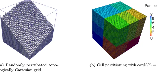
specific, two types of grid have been tested. The first one is a Cartesian mesh and the second one is obtained from the previous one by a random perturbation of its nodes leading to hexahedral cells with non planar faces. For the sake of clarity, a coarser randomly perturbed grid of size 323 is exhibited on the Figure 8(a), and its
partitioning is presented on the Figure 8(a).
(a) Randomly pertubated topo-logically Cartesian grid
(b) Cell partitioning with card(P) = 10
Figure 8. Randomly perturbed topologically Cartesian grid type used for the numerical validation.
In this test case, the parabolic equation is solved on the unit cube Ω = [0,1]3, with Dirichlet boundary
condition on ∂Ω, and an initial condition both defined by the function
u(x, y, z) = sin(2πx) sin(2πy) sin(2πz) + 4.
The time interval is given by [0,0.05] and is discretized using a constant time step of 0.001.
This numerical example has been run using the OpenMPI library version 1.4.5 on themeso-centre of Aix-Marseille University which provides a cluster architecture of 96 nodes each equipped with 12 cores and connected by an InfiniBand QDR communications link (see [2] for more details).
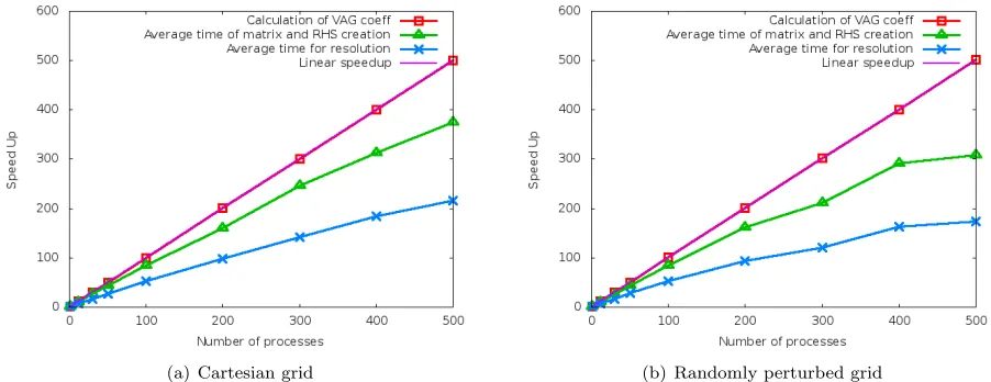
The Figure 9 exhibits the speed-up obtained with both types of grids with the following splitting of the run times:
(i) computation of the VAG transmissivities as discussed in the subsection 2.3,
(ii) creation of the PETSc objects, assembly of the matrix and of the right-hand side (denoted RHS), and computation of the Schur complement as described in the subsection 2.4,
(iii) computation of the discrete solution, including both the call to the linear solver of PETSc, and the calculation of the cell unknowns using (16).
minimum of 50000 cells for each process. This explains the decrease of the parallel efficiency in our case over a few tens of processes. All together, the results of the two test cases exhibit a rather good strong scalability of the code ComPASS which validates our implementation.
(a) Cartesian grid (b) Randomly perturbed grid
Figure 9. Speed-up study using two types of topologically Cartesian grids with 1283 cells and up to 500 processes. Speed Up : Sp(n proc) = Time(1proc)/Time(n proc); linear Speed up
Sp(n proc)=n.
4.
Conclusion and perspectives
The CEMRACS has offered an ideal framework to start in a collaborative project the development of the new code ComPASS adapted to the distributed parallelization of Finite Volume schemes on general unstructured meshes using various d.o.f. including typically cell, face or vertex unknowns. The parallelization is based on a classical domain decomposition approach with one layer of cells as overlap allowing to assemble the systems locally on each process. The code is adapted to fully implicit time integrations of evolution problems thanks to the connection with the PETSc library in order to solve the linear systems.
To simplify the implementation, at least in a first step, it has been decided to read and partition the mesh on a master process which distributes it to all processors in a preprocessing step. All the remaining computations are done in parallel. The code has been tested on a parabolic toy problem to evaluate its parallel efficiency on up to 500 processes. The results exhibit a rather good strong scalability of the CPU time with a typical behaviour of the parallel efficiency for implicit discretizations on a fixed mesh size.
This is clearly only the first step of development of a more advanced version of the code. In the near future, we intent first to improve the parallelization of the post-processing step of the code, and of course to include more physics starting with multiphase porous media flow applications.
Last but not least, this CEMRACS project has also offered to the youngest authors, the opportunity to learn MPI parallel programming and to work in a collaborative project using appropriate software engineering tools.
Acknowledgement
References
[1] DUNE – Distributed and Unified Numerics Environment.http://www.dune-project.org/. [2] Meso-centre of Aix-Marseille university.http://cbrl.up.univ-mrs.fr/~mesocentre/. [3] Metis.http://glaros.dtc.umn.edu/gkhome/views/metis.
[4] PETSc.http://www.mcs.anl.gov/petsc.
[5] The Trilinos Project.http://www.http://trilinos.sandia.gov/.
[6] I. Aavatsmark, T. Barkve, O. Bøe, and T. Mannseth. Discretization on non-orthogonal, curvilinear grids for multi-phase flow. in prov. of the 4th european conf. on the mathematics of oil recovery, 1994.
[7] B. Andreianov, F. Hubert, and S. Krell. Benchmark 3d: a version of the ddfv scheme with cell/vertex unknowns on general meshes. 2011.
[8] K. Aziz and A Settari.Petroleum reservoir simulation. Applied Science Publishers, 1979.
[9] F. Brezzi, K. Lipnikov, and V. Simoncini. A family of mimetic finite difference methods on polygonal and polyhedral meshes. Mathematical Models and Methods in Applied Sciences, 15(10):1533–1552, 2005.
[10] K.H. Coats. Implicit compositional simulation of single-porosity and dual-porosity reservoirs. InSPE Symposium on Reservoir Simulation, 1989.
[11] M.G. Edwards and C.F. Rogers. A flux continuous scheme for the full tensor pressure equation. in prov. of the 4th european conf. on the mathematics of oil recovery, 1994.
[12] R. Eymard, P. F´eron, T. Gallou¨et, C. Guichard, and R. Herbin. Gradient schemes for the stefan problem.submitted, 2012. preprinthttp://hal.archives-ouvertes.fr/hal-00751555.
[13] R. Eymard, T. Gallou¨et, and R. Herbin. Discretisation of heterogeneous and anisotropic diffusion problems on general non-conforming meshes, sushi: a scheme using stabilisation and hybrid interfaces.IMA J. Numer. Anal., 30(4):1009–1043, 2010. [14] R. Eymard, C. Guichard, and R. Herbin. Small-stencil 3d schemes for diffusive flows in porous media.M2AN Math. Model.
Numer. Anal., 46:265–290, 2012.
[15] R. Eymard, C. Guichard, R. Herbin, and R. Masson. Vertex-centred discretization of multiphase compositional darcy flows on general meshes.Computational Geosciences, pages 1–19, 2012.
[16] R. Eymard, G. Henry, R. Herbin, F. Hubert, R. Kl¨ofkorn, and G. Manzini. 3D benchmark on discretization schemes for anisotropic diffusion problems on general grids.Finite Volumes for Complex Applications VI Problems & Perspectives, pages 895–930, 2011.
[17] W. Gropp, E. Lusk, N. Doss, and A. Skjellum. A high-performance, portable implementation of the mpi message passing interface standard.Parallel computing, 22(6):789–828, 1996.
[18] W. Gropp, E. Lusk, and A. Skjellum.Using MPI: portable parallel programming with the message passing interface, volume 1. MIT press, 1999.
[19] Gilles Grospellier and Benoit Lelandais. The arcane development framework. In Proceedings of the 8th workshop on Parallel/High-Performance Object-Oriented Scientific Computing, POOSC ’09, pages 4:1–4:11, New York, NY, USA, 2009. ACM.
[20] G.R. Luecke, Y. Zou, J. Coyle, J. Hoekstra, and M. Kraeva. Deadlock detection in mpi programs.Concurrency and Compu-tation: Practice and Experience, 14(11):911–932, 2002.