https://doi.org/10.5194/gmd-10-2321-2017 © Author(s) 2017. This work is distributed under the Creative Commons Attribution 3.0 License.
A Bayesian posterior predictive framework for weighting ensemble
regional climate models
Yanan Fan1, Roman Olson2, and Jason P. Evans3
1School of Mathematics and Statistics, UNSW, Sydney, Australia
2Department of Atmospheric Sciences, Yonsei University, Seoul, South Korea
3Climate Change Research Centre and ARC Centre of Excellence for Climate System Science, UNSW, Sydney, Australia
Correspondence to:Yanan Fan ([email protected])
Received: 28 November 2016 – Discussion started: 4 January 2017
Revised: 17 May 2017 – Accepted: 22 May 2017 – Published: 23 June 2017
Abstract. We present a novel Bayesian statistical approach to computing model weights in climate change projection ensembles in order to create probabilistic projections. The weight of each climate model is obtained by weighting the current day observed data under the posterior distribution admitted under competing climate models. We use a lin-ear model to describe the model output and observations. The approach accounts for uncertainty in model bias, trend and internal variability, including error in the observations used. Our framework is general, requires very little problem-specific input, and works well with default priors. We carry out cross-validation checks that confirm that the method pro-duces the correct coverage.
1 Introduction
Regional climate models (RCMs) are powerful tools to pro-duce regional climate projections (Giorgi and Bates, 1989; Christensen et al., 2007; van der Linden and Mitchell, 2009; Evans et al., 2013, 2014; Mearns et al., 2013; Solman et al., 2013; Olson et al., 2016b). These models take climate states produced by global climate models (GCMs) as bound-ary conditions, and solve equations of motion for the atmo-sphere on a regional grid to produce regional climate pro-jections. The main advantages of RCMs over GCMs are in-creased resolution, more parsimony in terms of representing sub-grid-scale processes, and often improved modelling of spatial patterns, particularly in regions with coastlines and considerable topographic features (e.g. van der Linden and Mitchell, 2009; Prömmel et al., 2010; Feser et al., 2011).
Current computing power is now allowing for ensembles of regional climate models to be performed, allowing for sampling of model structural uncertainty (Christensen et al., 2007; Giorgi and Bates, 1989; van der Linden and Mitchell, 2009; Mearns et al., 2013; Solman et al., 2013).
Along with these ensemble modelling studies, methods for extracting probabilistic projections have followed (Buser et al., 2010; Fischer et al., 2012; Kerkhoff et al., 2015; Olson et al., 2016a; Wang et al., 2016). While these studies all take a Bayesian approach, the implementations differ. For exam-ple, Buser et al. (2010) and Kerkhoff et al. (2015) model both the RCM output and the observations as a function of time. However, this implementation uses too many parame-ters to be applicable to short (e.g. 20-year) time series com-mon in regional climate modelling. Furthermore, the results are affected by climate model convergence: the output from the outlier models is pulled towards clusters of converging models. The Wang et al. (2016) method is applicable to rela-tively short time series; however, convergence still influences model predictions.
smooth-ing choice is not explicitly considered. Second, in the pro-jection stage the Olson et al. (2016a) implementation does not fully account for the uncertainty in model biases and in standard deviation of the model–data residuals.
Several authors have shown that in many regions, future changes are positively correlated with present-day internal variability in the models: see Buser et al. (2009) and Hut-tunen et al. (2017). This means that knowing internal vari-ability may provide important information and potentially improve future projections. While previous works have in-cluded information from internal variability in their statisti-cal model, the information was not used to directly penalise the models for getting the internal variability wrong: see for example Buser et al. (2010) and Kerkhoff et al. (2015). Olson et al. (2016a) was the first attempt to incorporate this infor-mation via penalising model priors. However, the priors were chosen ad hoc. A fundamental improvement of this work is weighting the models not just by their performance in terms of the mean, but also in terms of the internal variability in a principled way.
In this article, we propose a new method to obtain model weights using raw model output, so the method better ac-counts for model output uncertainty. Our framework allows us to compute weights efficiently, simultaneously penalising for model bias, deviations in trend and model internal vari-ability. One of the main advantages of the current approach is that improper and vague priors for the model parameters can be used, which makes implementation of the method much more straightforward. In the Olson et al. (2016a) framework, subjective and informative parameter choices are required. Such choices impact strongly on the resulting weights and inference. In addition, their framework cannot accommodate improper priors since they need to be able to sample directly from the prior.
Below the Bayesian methodology developed is described followed by a Markov chain Monte Carlo (MCMC) method to obtain solutions for the posterior distributions. The tech-nique is then applied to a regional climate model ensemble and compared with results found in previous work (Olson et al., 2016a).
2 Posterior predictive weighting
In this section, we introduce the Bayesian methodology for weighting model output based on current day observations. The framework we describe below is not limited to any par-ticular distributional form, although the analysis presented is based on the univariate normal distribution. We have also im-plemented the same procedure using the asymmetric Laplace distribution for median regression to obtain robust estima-tors for our analyses, but we have excluded them from pre-sentation as the procedure produced similar results to that of the normal error assumption (indicating no major violations from normality).
−2 −1 0 1 2
0e+00
1e−12
2e−12
3e−12
4e−12
5e−12
µ
W
eight
0 1 2 3 4 5
0e+00
1e−12
2e−12
3e−12
4e−12
5e−12
6e−12
σ
W
eight
Figure 1.Pictorial representation of the weight distribution onµ
andσ.
We suppose that current day observations are denoted as yt, wheret=1, . . ., T is a set of indices for time. We assume
that the present-day observations over time can be described by
yt=ap+bp(t−t1)+t (1)
wheret ∼N (0, σp),t=t0, . . .t0+T, andt0is the first year
that the observation is available, andt1=t0+T /2.
Formu-lating the equation in terms oft1 allows us to interpretap
as the mean value of the observations. This model is rea-sonable for the type of short time series temperature data that we consider. We assume that the datayt are
indepen-dent between observations. Letxtm, t=1, . . ., T denote data generated by themth model over the same time period, where m=1, . . ., M, and we assume that each set of model outputs can be adequately modelled by
xtm=am+bm(t−t1)+t (2)
withi∼N (0, σm). Again,xts are assumed independent.
The parameters am, bm, σm can be obtained under the
Bayesian paradigm by first specifying a prior distribution p(am, bm, σm), and the posterior distribution given dataxm
is subsequently obtained via the Bayes rule,
p(am, bm, σm|xm)∝L(xm|am, bm, σm)p(am, bm, σm), (3)
subjec-Figure 2.New South Wales planning regions, the ACT and the state of Victoria.
tive analyses. Vague priors are sometimes considered prefer-able when data contain sufficient information or when sub-jective knowledge is uncertain. Conjugate analyses for cer-tain classes of models, including Gaussian error models, are often possible, leading to analytical forms for the posterior distributions. In this work, we choose to present the results with non-standard priors, and use MCMC for computation. This approach is much easier when extending to more com-plex modelling scenarios.
We would like to weight the models based on the similar-ity of outputxtmto the observation data. We note that a model that performs well under recent conditions does not guaran-tee that it will perform well under future climate conditions, but we assume that good performance under recent condi-tions is an indication of reliable performance in future cli-mates. This translates to preferring models whose parameters am, bm, σmare similar toap, bp, σp. In practiceσphas
addi-tional terms, due to instrumental and gridding error associ-ated with collecting observational data. This additional error is not reflected in the model output. Jones et al. (2009) per-formed error analyses for 2001–2007 for Australian climate data, and found that the root mean squared error for monthly temperature data ranges between 0.5 and 1 K. For our analy-ses of seasonally averaged temperature data in Sect. 2.2, we set the additional error to be δ=0.5 K. Resulting weights were largely insensitive to values ofδbetween 0.5 and 1.
Finally, we define the weight for each modelmto be of the form
wm= Z
L(y|am, bm, q
σ2
m+δ2)p(am, bm, σm|xm)damdbmdσm (4) where L(y|am, bm,
p
σ2
m+δ2) denotes the likelihood of
observational data y, given the parameters of the mth model, am, bm and σm. The weight wm fully accounts for
the uncertainties associated with the estimates of am, bm
and σm, by averaging over the posterior distribution of
p(am, bm, σm|xm). Clearly, the right-hand side of Eq. (4) will
be larger ifam, bmand p
σ2
m+δ2are similar to ap, bp and
σp, i.e. if the distributions ofy andxm are similar (up to a
difference of observational errorδ). We term these weights the posterior predictive weights. Note that Eq. (4) is simply the marginal likelihoodp(y|xm), i.e. the probability of ob-serving dataygivenxm, averaging over any model parameter
uncertainties. The termam and its deviation fromap in the
observation model can be considered as penalising bias be-tween model output and observation, the deviation bebe-tween bmandbp can be thought of as a penalty for trend, and the
termsσm andσp account for the differences of model and
observation internal variability.
The ensemble models can now be combined into a single posterior model, using the weights
p(aBMA, bBMA, σBMA|x1, . . ., xM)
=
M X
m=1
wmp(am, bm, σm|xm). (5)
The above expression gives us an ensemble estimate for the posterior distribution of the parameters fora,bandσ from theM model outputs, and we denote these asaBMA,bBMA
andσBMA. Note that the weights should be normalised by PM
m=1wm=1.
In order to understand this weight, we suppose for the mo-ment that the dataycome from, say, aN (0,1). Suppose also thatxmcomes fromN (µ, σ ). Then if the posterior distribu-tions of µ andσ are centered around 0 and 1,xm should be assigned a higher weight. As the values ofµandσ di-verge away from 0 and 1, we should see a decrease in the respective weights. Figure 1 plots the likelihood of 50 simu-latedyvalues fromN (0,1)distribution, the left panel shows the weights for a fixed value ofµ= −2, . . .,2 and σ=1, and the right panel shows the weights for a fixed value of σ=0.01, . . .,5 withµ=0. The figure corresponds to a sin-gle term inside the weight Eq. (4), where am,I, bm,I
corre-spond toµand
q
σm,2I+δ2corresponds toσ. See also Eq. (6)
below. The figure shows the changes in the weight, as param-eter values move away from the true values of 0 and 1. In the case of single fixed values ofµ andσ, the weights simply correspond to the likelihood at these values. In practice, the weights in Eq. (4) average over the set of posterior values of µandσ.
1 3 5 7 9 11 (a) Weight
Models
0.0
0.2
0.4
1 3 5 7 9 11 (b) Weight intercept
0.00
0.10
0.20
1 3 5 7 9 11 (c) Weight slope
0.00 0.06 0.12 ● ● ●● ●●● ● ● ● ● ●● ● ● ● ● ● ●
10 15 20 25
18
20
22
24
26
(d) Model 1, 2, 3
Years O bs ● ● ●● ●●● ● ● ● ● ●● ● ● ● ● ● ●
10 15 20 25
18
20
22
24
26
(e) Model 4,5,6
Years O bs ● ● ●● ●●● ● ● ● ● ●● ● ● ● ● ● ●
10 15 20 25
18
20
22
24
26
(f) Model 7, 8, 9
O bs ● ● ●● ● ●● ● ● ● ● ●● ● ● ● ● ● ●
10 15 20 25
18
20
22
24
26
(g) Model 10, 11, 12
Years O bs ● ● ●● ● ●● ● ● ● ● ●● ● ● ● ● ● ●
10 15 20 25
18
20
22
24
26
(h) Weighted fit
Years O bs ● ● ●● ● ●● ● ● ● ● ●● ● ● ● ● ● ●
10 15 20 25
18 20 22 24 26 Years
(i) Weighted fit (I/S)
Years
O
bs
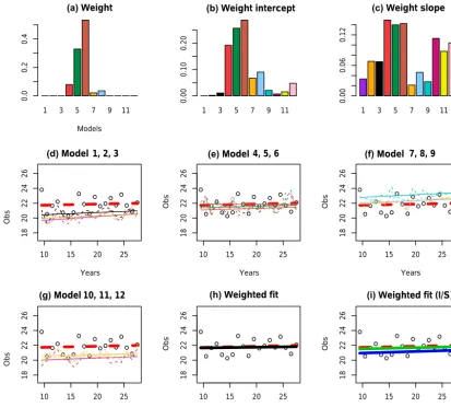
Figure 3.Results for the CC region of south-eastern Australia, in the DJF season. Top row: weightswmof 12 models based on Eq. (4) (L), Eq. (8),wm,I(M) and Eq. (9)wm,T(R). Each triplet represents a GCM (MIROC3.2, ECHAM5, CCCMA3.1, and CSIRO-Mk3.0). Middle row and first plot of last row: fitted observations according to Eq. (1) (red dashed line) and fitted model output according to Eq. (2) for 12 models. Last row: weighted fit based onwmin solid black line (M), weighted fit based onwm,Iin solid green line and weighted fit based on
wm,Tin solid blue line (R).
between future climate and future model output behaves in a similar way to the relationship between present-day climate and present-day model output. We consider that there is a perfect model that has the same parameters (intercept, slope and standard deviation) in both the present and the future. We then compute the probability that any modelmis this perfect model, based on present-day data. These assumptions can be seen as an informative prior on the parameters governing fu-ture observations, although these parameters are not explic-itly modelled.
2.1 Computation
The procedure for the calculation of weights is designed to be applicable regardless of the distributional forms cho-sen to model the data. In most cases, the posterior
distri-butionsp(am, bm, σm|xm)in Eq. (3) will be analytically
1 3 5 7 9 11
(a) Weight
Models
0.0
0.1
0.2
0.3
0.4
1 3 5 7 9 11
(b) Weight intercept
0.00
0.10
1 3 5 7 9 11
(c) Weight slope
0.00
0.10
0.20
●
●● ● ●
● ● ● ●
● ●
● ●●
● ●
● ●
●
10 15 20 25
24
28
32
(d) Model 1,2, 3
Years
O
bs ●
●● ● ●
● ● ● ●
● ●
● ●●
● ●
● ●
●
10 15 20 25
24
28
32
(e) Model 4,5,6
Years
O
bs ●
●● ● ●
● ● ● ●
● ●
● ●●
● ●
● ●
●
10 15 20 25
24
28
32
(f) Model 7, 8, 9
Years
O
bs
●
●● ● ●
● ● ● ●
● ●
● ●●
● ●
● ●
●
10 15 20 25
24
28
32
(g) Model 10, 11, 12
Years
O
bs ●
●● ● ●
● ● ● ●
● ●
● ●●
● ●
● ●
●
10 15 20 25
24
28
32
(h) Weighted fit
Years
O
bs ●
●● ● ●
● ● ● ●
● ●
● ●●
● ●
● ●
●
10 15 20 25
24
28
32
(i) Weighted fit (I/S)
Years
O
bs
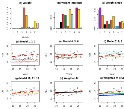
Figure 4.Results for the FW region of south-eastern Australia, in the DJF season. Top row: weightswmof 12 models based on Eq. (4) (L), Eq. (8),wm,I(M) and Eq. (9)wm,T(R). Each triplet represents a GCM (MIROC3.2, ECHAM5, CCCMA3.1, and CSIRO-Mk3.0). Middle row and first plot of last row: fitted observations according to Eq. (1) (red dashed line) and fitted model output according to Eq. (2) for 12 models. Last row: weighted fit based onwmin solid black line (M), weighted fit based onwm,Iin solid green line and weighted fit based on
wm,Tin solid blue line (R).
In addition to obtaining simulations from the posteriors of the M ensemble models, the weight calculation in Eq. (4) also involves an intractable integral, which we can approxi-mate using standard Monte Carlo
wm≈ X
am,I,bm,I,σm,I
L(y|am,I, bm,I, q
σm,2I+δ2) (6)
whereL(y|am,I, bm,I, q
σm,2I+δ2)denotes the likelihood of
y under theith sample ofam,I, bm,I andσm,Ifrom the
pos-terior distributionp(am, bm, σm|xm). Thus, the 4500 MCMC
samples obtained for each model are then used to compute the Monte Carlo sum in Eq. (6). Again, the weights should be normalised by the constraintPM
m=1wm=1.
Finally, the predictive distribution for the future cli-mateytf, t=1, . . ., T0, given future model output denoted as
xf,1, . . ., xf,m, is defined as p(y1f, . . ., yTf0|xf,1, . . ., xf,M)=
Z
p(y1f, . . ., yTf0|aBMAf , bfBMA, σBMAf )
p(aBMAf , bfBMA, σBMAf |xf,1, . . ., xf,M)
dafBMAdbfBMAdσBMAf . (7)
2.2 Application
1 3 5 7 9 11
D:eight
0odels
0.0
0.2
0.4
1 3 5 7 9 11
E:eight intercept
0.0
0.2
0.4
1 3 5 7 9 11
F:eight slope
0.00
0.10
● ● ● ● ● ●●
●● ●● ●
● ●●
●
● ●
● ●
10 15 20 25
14
16
18
20
22
G0odel 1,2, 3
<ears
2
bs ● ● ● ●
● ●● ●●
●● ● ●
●● ●
● ●
● ●
10 15 20 25
14
16
18
20
22
H0odel 4,5,6
<ears
2
bs ● ● ● ●
● ●● ●●
●● ● ●
●● ●
● ●
● ●
10 15 20 25
14
16
18
20
22
I0odel 7, 8, 9
<ears
2
bs
● ● ● ● ● ●●
●● ●● ●
● ●●
●
● ●
● ●
10 15 20 25
14
16
18
20
22
(g) Model 10, 11, 12
<ears
2
bs ● ● ● ●
● ●● ●●
●● ● ●
●● ●
● ●
● ●
10 15 20 25
14
16
18
20
22
(h) Weighted fit
<ears
2
bs ● ● ● ●
● ●● ●●
●● ● ●
●● ●
● ●
● ●
10 15 20 25
14
16
18
20
22
(i) Weighted fit (I/S)
<ears
2
bs
Figure 5.Results for the CWO region of south-eastern Australia, in the MAM season. Top row: weightswmof 12 models based on Eq. (4) (L), Eq. (8),wm,I(M) and Eq. (9)wm,T (R). Each triplet represents a GCM (MIROC3.2, ECHAM5, CCCMA3.1, and CSIRO-Mk3.0). Middle row and first plot of last row: fitted observations according to Eq. (1) (red dashed line) and fitted model output according to Eq. (2) for 12 models. Last row: weighted fit based onwmin solid black line (M), weighted fit based onwm,Iin solid green line and weighted fit based onwm,Tin solid blue line (R).
CCCMA3.1, and CSIRO-Mk3.0) with three versions of the WRF modelling framework (which we call R1, R2, and R3, Skamarock et al., 2008) that differ in parameterisations of radiation, cumulus physics, surface physics, and planetary boundary layer physics. NARCliM output has been evaluated in terms of its ability to reproduce the observed mean cli-mate (Ji et al., 2016; Olson et al., 2016b; Grose et al., 2015), climate extremes (Cortés-Hernández et al., 2015; Perkins-Kirkpatrick et al., 2016; Walsh et al., 2016; Kiem et al., 2016; Sharples et al., 2016), and important regional climate phe-nomena (Di Luca et al., 2016; Pepler et al., 2016). These studies demonstrate that while the downscaling has provided added value (Di Luca et al., 2016), a range of model errors are present within the ensemble. For the analysis, we fo-cus on seasonal–mean temperature differences as modelled by the inner NARCliM domain RCMs between years 1990–
2009 (present) and 2060–2079 (far future). We discard partial seasons from the analysis.
Here we average the temperatures over south-eastern Aus-tralian regions that include New South Wales (NSW) plan-ning regions, ACT, and Victoria; see Fig. 2. Corresponding temperature observations are derived from the AWAP project (Jones et al., 2009). The models are generally cooler than the observations; however, in many cases the observations span the mean model climate.
In addition to computing weights of the form in Eq. (4), we also compute two variants of the weight: one based on penal-ising only the interceptam and internal variabilityσm, and
0 1 2 3 4 5
0.0
0.4
0.8
1.2
FW
●● ●●●●●●●●● ●x
0 1 2 3 4 5
0.0
0.5
1.0
1.5
NENW
● ● ●●●●x●●●●●●
0 1 2 3 4 5
0.0
0.5
1.0
1.5
NC
● ● ●●●●x●●●●●●
0 2 4
0.0
0.5
1.0
1.5
Hun
●● ●●●●x●●●●●●
1 2 3 4 5
0.0
0.5
1.0
1.5
CWO
●● ●●●●x●●●●●●
0 1 2 3 4 5
0.0
0.4
0.8
1.2
MM
●●●●●●●●●● ● ● x
1 2 3 4 5
0.0
0.5
1.0
1.5
CC
●● ●●●●●●●●● ●x
1 2 3 4
0.0
0.5
1.0
1.5
2.0
Msyd
●● ●●●●●x●●●●●
1 2 3 4
0.0
0.5
1.0
1.5
2.0
Ill
●● ●●●●●●●●● ●x
0 1 2 3 4
0.0
0.5
1.0
1.5
SET
●●●●●●●●●●● ●x
1 2 3 4
0.0
0.5
1.0
1.5
ACT
●●●●●●●●●●● ●x
0 1 2 3 4
0.0
0.5
1.0
1.5
Victoria
●●●●● ●●● ● ● ● ● x
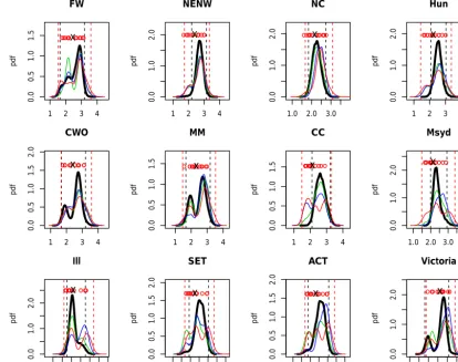
Figure 6.Posterior predictive projections of DJF temperature change in 2060–2079 compared to 1990–2009 for regions in south-eastern Australia. Black lines correspond towmweights, green lines towm,Iweights and blue lines towm,Tweights. Red lines are results from Olson et al. (2016a). Black vertical lines represent 95 % credible intervals, and red vertical lines represent the 95 % credible intervals obtained by Olson et al. (2016a). Circles represent the difference between the changes in temperature using the individual models. Black crosses indicate the simple ensemble mean of the changes in temperature.
Eq. (4) to wm,I=
Z
L(y|am, bp, q
σ2
m+δ2)p(am, σm|xm)damdσm (8)
or wm,T=
Z
L(y|ap, bm, q
σ2
m+δ2)p(bm, σm|xm)dbmdσm (9)
wherewm,Ipenalises models with large biases and wrong in-ternal variability, andwm,Tpenalises models with the wrong trend and internal variability. Note that our proposed weight wm penalises bias, trend and internal variability simultane-ously. The weightswm,Iandwm,Tcan be computed by fit-ting the observation data to the model in Eq. (1) to obtain estimates for ap andbp, and using only the posterior
sam-ples ofam, bmandσmto complete the calculation.
Figure 3 shows the weight calculation of each model based on Eq. (4), for the CC region in season DJF. We used the observed data and the corresponding model output for the
years 1990–2009. One can see how the three different types of weights behave relative to the bias and slope of the model output. For example, in Fig. 3, models 1,2,3 (left figure, middle row) and 10, 11, 12 (left figure, bottom row) have large bias compared to the other models; consequently,wm andwm,Igive these models almost no weight. On the other hand these models simulated the trend well, and are preferred bywm,T.
The weighted fits are shown in the last two plots in the bottom row of Fig. 3. The black line is computed usingwm, according to
ˆ yt=
M X
m=1
wm(am+bm·t ) (10)
wheream and bm are taken as the posterior means of the
1 2 3 4
0.0
0.5
1.0
1.5
FW
●● ●●●●●●●●● ● x
1 2 3 4
0.0
1.0
2.0
NENW
● ● ●●●●x●●●●●●
1.0 2.0 3.0
0.0
1.0
2.0
NC
●● ●●●●x●● ●●●●
1 2 3 4
0.0
1.0
2.0
Hun
●● ●●●●x●●●●●●
1 2 3 4
0.0
0.5
1.0
1.5
2.0
CWO
●● ●●●●x●●●●●●
1 2 3 4
0.0
0.5
1.0
1.5
MM
● ●●●●●●●●● ● ● x
1 2 3 4
0.0
0.5
1.0
1.5
CC
●● ●●●●●●●●● ●x
1.0 2.0 3.0 4.0
0.0
1.0
2.0
Msyd
● ● ●●●●●x●●●●●
1.0 2.0 3.0 4.0
0.0
1.0
2.0
Ill
● ● ●●●●●● ●●● ●x
1.0 2.0 3.0 4.0
0.0
0.5
1.0
1.5
2.0
SET
● ●●●●●●●●●● ● x
1.0 2.0 3.0 4.0
0.0
0.5
1.0
1.5
2.0
ACT
●●●●●●●●●●● ●x
0.5 1.5 2.5 3.5
0.0
1.0
2.0
Victoria
●●●●● ●●● ● ● ● ● x
Figure 7.Bootstrapped weighted projections of DJF temperature change in 2060–2079 compared to 1990–2009 for regions in south-eastern Australia. Black lines correspond towmweights, green lines towm,Iweights and blue lines towm,Tweights. Red lines are results from Olson et al. (2016a). Black vertical lines represent 95 % credible intervals, and red vertical lines represent the 95 % credible intervals obtained by Olson et al. (2016a). Circles represent the difference between the changes in temperature using the individual models. Black crosses indicate the simple ensemble mean of the changes in temperature.
Table 1.Mean squared error and 95 % coverage probabilities for the three sets of weights.
DJF MAM JJA SON
MSE Cov MSE Cov MSE Cov MSE Cov
wm 48.43 0.938 14.44 0.958 14.15 0.910 41.86 0.917
wm,I 52.06 0.965 21.34 0.979 17.89 0.944 43.55 0.951
wm,T 56.93 0.993 30.74 0.979 20.45 0.972 39.79 1.000
are similar to wm,I, and better than wm,T in this case. We note that there are dependencies between the RCMs driven by the same GCM. Our weight calculation does not model this dependence. So if different GCMs drive a different num-ber of RCMs, the weights will over-represent some models but not others. While for most cases, the weights given by wm,I provide similar weighted fits towm, Fig. 4 (showing the FW region for season DJF) demonstrates the instances where the weighted fit produced by wm,I is clearly worse than wm. The green line in the final plot shows that wm,I
produces a fit which is very close to the observation at the intercept but fails to capture the trend. This is unsurprising since this weight penalises deviations ofamtoap. Similarly,
1 2 3 4
0.0
1.0
2.0
CC
X
0 1 2 3 4
0.0
0.5
1.0
1.5
2.0
CC
X
0 1 2 3 4
0.0
0.5
1.0
1.5
CC
X
0 1 2 3 4 5
0.0
0.5
1.0
1.5
CC
X
1 2 3 4
0.0
0.5
1.0
1.5
CC
X
1 2 3 4 5
0.0
0.5
1.0
1.5
CC
X
0 1 2 3 4
0.0
1.0
2.0
CC
X
1 2 3 4
0.0
1.0
2.0
CC
X
1 2 3 4
0.0
1.0
2.0
CC
X
0 1 2 3 4
0.0
0.5
1.0
1.5
CC
X
0 1 2 3 4
0.0
0.5
1.0
1.5
2.0
CC
X
0 1 2 3 4
0.0
0.5
1.0
1.5
CC
X
Figure 8.Cross validation of weighted projections of DJF temperature change in 2060–2079 compared to 1990–2009 for region CC in south-eastern Australia. Black lines correspond towmweights; green lines correspond towm,Iweights andwm,Tweights. Each plot represents the weighted posterior predictive distribution of temperature change using the currentith model output as observation and the remaining 11 models are weighted. Vertical lines represent 95 % credible intervals. Crosses indicate the actual changes between the future model output and the current model output of theith model.
spread out, giving high weights to models 1 and 2, which have large biases but capture the trend well. The weightswm allocate most weight to models 6 and 7. Both models closely follow the shape of the observed data. In fact, in terms of trend, the weightswm,Tcan capture more of the increase in trend better thanwm, this was the case in some of the regions in the SON season. A more formal evaluation of the three different weights will be carried out later in this section.
For seasons JJA and MAM, weights wm andwm,I were quite similar in all regions. These weights gave very close fits to the observation model, whilewm,Tcaptured the trend well but gave biased fits to the observation. Generally for these two seasons, fewer models had non-neglible weights compared with DJF and SON. In DJF and SON, the weights were distributed more evenly across the models. This sug-gests that some of the individual models in JJA and MAM were performing strongly. Interestingly for MAM, the two models that dominated most regions are models 8 and 9; see for example the results for region CWO in Fig. 5. We can see
the goodness of fit of these two models individually (see sec-ond row, right plot), and clearly they were markedly better than the other competing models.
The corresponding posterior predictive distribution of pro-jections of change in temperature for season DJF over the different regions in south-eastern Australia are plotted in Fig. 6. The pdfs show the mean temperature change in the period 2060–2079 compared to 1990–2009. In order to ob-tain the posterior predictive projection pdf, we begin by first fitting MCMC for each future model output for the period 2060–2079, to obtain the posterior distribution of p(amf, bfm, σmf|xm). Here we obtained 5000 posterior samples ofamf.bfmandσmf. We then obtain 10 000 random samples for each pdf. Each sample is obtained as follows.
1. With probabilitywm, randomly select a sample from the posteriors ofamfbfmandσmf, sayam,f Ibm,f Iandσm,f I. 2. Simulate a predictive temperature seriesytfaccording to
for t=2060, . . .,2079 and t1=2069.5. This process
produces the posterior predictive samplesytfaccording to Eq. (7).
3. Compute current model estimateyˆtm=am+bm·(t−t1),
for t=1990, . . .,2009 and t1=1999.5 wheream and
bmare posterior means based on modelmand current
model outputxm.
4. Compute the mean of the differences between future predictionytfandyˆtm.
This process produces the posterior predictive distributions for the mean difference between the posterior predictive sam-plesytfand the current estimate of climate.
We present the results for season DJF in Fig. 6. The black lines in Fig. 6 correspond to the pdf given bywm, the green lines correspond to wm,I and the blue lines correspond to wm,T. The red circles indicate the difference between the means ofyˆt andyˆtffrom each of the 12 models; the cross
dicates the mean of these differences. Black vertical lines in-dicate the 95 % credibility interval for predictions made with wm(black line). We can see that the pdfs based onwmand wm,Iare similar to each other, while the ones given bywm,T deviate substantially from the other two. We also superim-posed the pdf obtained in Olson et al. (2016a) in red for com-parison. The corresponding 95 % credible interval is shown in red vertical lines. It can be seen that our method gener-ally provides a more precise prediction interval. In fact, to properly compare the two predictive distributions, we com-pute the posterior predictive distribution using the method described by Olson et al. (2016a). Unlike our posterior pre-dictive pdf, the pdf in Olson et al. (2016a) was obtained by bootstrapping the errors, and does not account for the un-certainty in the parameter estimates of am, bm andσm. To
properly compare the effect of the different weights between our method and that of Olson et al. (2016a), we also show in Fig. 7 the bootstrapped pdf. Here the red line indicates the pdf using Olson et al. (2016a) weights with the 95 % credible interval shown in red vertical lines, and here we can see that Olson et al. (2016a) generally produce significantly larger credible intervals than our approach.
The incident of bimodality or multimodality is reduced in our approach compared to Olson et al. (2016a), suggesting a smoother mixing of models induced by our approach. Our approach generally produced sharper, more definite peaks in the posterior pdf. This could be due to the fact that our penal-isation is done simultaneously, whereas Olson et al. (2016a) consider the penalty for bias and internal variability sepa-rately.
In order to assess the ensemble pdf, we performed a series of cross-validation checks. For each region at a given sea-son, we have 12 current model outputs and 12 future model outputs. We select 1 of the models, mi, and treat the
cur-rent model output formi as the truth, and weigh the
remain-ing 11 models. We then cycle through all 12 models, settremain-ing
mi =1, . . .,12. Figure 8 shows the weighted projections for
region CC in season DJF, each plot corresponding to using 1 of the 12 models as truth.
Table 1 shows the empirical coverage probabilities based on 144 sets of cross-validation datasets for each region, DJF, MAM, JJA and SON. The coverage probabilities are com-puted by counting the number of times the true mean change in temperature falls inside the 95 % credibility intervals, taken as the 0.025th and 0.975th quantile values of the pos-terior predictive samples. Each weighting method produces a different set of credibility intervals. We see from the ta-ble that bothwmandwm,Iperform quite close to the nom-inal level at 95 %, but the pdfs given by the weightwm,T are a little too large. Finally, we also computed the mean squared error for each season: this is calculated as the aver-age squared difference between the posterior predictive sam-ple and the true value. The sums over all regions and all cross-validation sets are reported in Table 1. Overall, the weightswmperformed consistently well in this respect.wm outperformswm,Iin all seasons. The poorer performance of wm,Tis largely due to the large biases in thewm,Tmodels. One possibility of makingwm,Tmodels more useful is to per-form some kind of post hoc bias correction to the weighted estimates.
3 Conclusions
In this article we have introduced a new framework for com-puting Bayesian model weights. Our framework is novel, and requires minimal expert knowledge of model parame-ters. The fact that we do not require subjective expert prior knowledge makes the method more robust, since prior elic-itation can sometimes be difficult, and different priors can lead to different conclusions.
We provided two alternative weight specifications under the same framework to aid interpretation of our weighting. One of the weights favours models with intercept terms that are close to the observation intercept. This weight does not penalise for trend deviations very well. An alternative weight which does not penalise for the intercept term can capture trend in the model very well. Both alternatives have defi-ciencies, and our proposed weight is a combination of the two. However, there are other potential avenues to explore with these alternative weights. For instance, for the weights based on trend and internal variability, it can be seen that the weighted model can capture trend extremely well but fails to account for bias, but applying some kind of post hoc bias correction may be a fruitful direction to pursue.
Fi-nally, our model weighting framework is not restricted to data from univariate normal distributions, or linear models. This approach could be extended to handle dependent Gaus-sian data via a multivariate normal distribution, as well as non-linear and non-normal models.
Code and data availability. Code and data for the analyses carried out in this article are available in the Supplement.
The Supplement related to this article is available online at https://doi.org/10.5194/gmd-10-2321-2017-supplement.
Competing interests. The authors declare that they have no conflict of interest.
Acknowledgements. This work was supported by the National Research Foundation of Korea Grant funded by the Korean Government (MEST) (NRF-2009-0093069).
Edited by: James Annan
Reviewed by: Hans R. Künsch and one anonymous referee
References
Bhat, K. S., Haran, M., Terando, A., and Keller, K.: Cli-mate Projections Using Bayesian Model Averaging and Space-Time Dependence, J. Agric. Biol. Envir. S., 16, 606?628, https://doi.org/10.1007/s13253-011-0069-3, 2011.
Buser, C. M., Künsch, H. R., Lüthi, D., Wild, M., and Schär, M. C.: Bayesian multi-model projections of climate: bias assumptions and interannual variability, Clim. Dynam., 33, 849–868, 2010. Buser, C. M., Künsch, H. R., and Schär, C.: Bayesian multi-model
projections of climate: generalization and application to EN-SEMBLES results, Climate Res., 44, 227–241, 2010.
Christensen, J. H., Carter, T. R., Rummukainen, M., and Amana-tidis, G.: Evaluating the performance and utility of regional cli-mate models: the PRUDENCE project, Climatic Change, 81, 1– 6, https://doi.org/10.1007/s10584-006-9211-6, 2007.
Cortés-Hernández, V. E., Zheng, F., Evans, J. P., Lambert, M., Sharma, A., and Westra, S.: Evaluating regional climate mod-els for simulating sub-daily rainfall extremes, Clim. Dynam., 47, 1613–1628, https://doi.org/10.1007/s00382-015-2923-4, 2015. Di Luca, A., Evans, J. P., Pepler, A., Alexander, L. V., and Argüeso,
D.: Australian East Coast Lows in a Regional Climate Model en-semble, Journal of Southern Hemisphere Earth Systems Science, 66, 108–124, 2016.
Di Luca, A., Argüeso, D., Evans, J. P., de Elia, R., and Laprise, R.: Quantifying the overall added value of dy-namical downscaling and the contribution from different spatial scales, J. Geophys. Res.-Atmos., 121, 1575–1590, https://doi.org/10.1002/2015JD024009, 2016.
Duan, Q., Ajami, N. K., Gao, X., and Sorooshian, S.: Multi-model ensemble hydrologic prediction using Bayesian model averaging, Adv. Water Resour., 30, 1371–1386, https://doi.org/10.1016/j.advwatres.2006.11.014, 2007. Evans, J. P., Fita, L., Argüeso, D., and Liu, Y.: Initial NARCliM
Evaluation, in MODSIM2013, 20th International Congress on Modelling and Simulation. Modelling and Simulation Society of Australia and New Zealand, December 2013, Adelaide, Aus-tralia, 2013.
Evans, J. P., Ji, F., Lee, C., Smith, P., Argüeso, D., and Fita, L.: Design of a regional climate modelling projection ensem-ble experiment – NARCliM, Geosci. Model Dev., 7, 621–629, https://doi.org/10.5194/gmd-7-621-2014, 2014.
Feser, F., Rrockel, B., von Storch, H., Winterfeldt, J., and Zahn, M.: Regional climate models add value to global model data: a review and selected examples, B. Am. Meteorol. Soc., 92, 1181–1192, 2011.
Fischer, A. M., Weigel, A. P., Buser, C. M., Knutti, R., Kün-sch, H. R., Liniger, M. A., Schär, C., and Appenzeller, C.: Climate change projections for Switzerland based on a Bayesian multi-model approach, Int. J. Climatol., 32, 2348– 2371, https://doi.org/10.1002/joc.3396, 2012.
Gilks, W. R., Richardson, S., and Spiegelhalter, D. J.: Markov Chain Monte Carlo in Practice, Chapman and Hall, 512 pp., 1996. Giorgi, F. and Bates, G. T.: The Climatological Skill of a
Regional Model over Complex Terrain, Mon. Weather Rev., 117, 2325–2347, https://doi.org/10.1175/1520-0493(1989)117<2325:TCSOAR>2.0.CO;2, 1989.
Giorgi, F., Jones, C., and Asrar, G. R.: Addressing climate informa-tion needs at the regional level: the CORDEX framework, WMO Bull., 58, 175–183, 2009.
Goes, M., Urban, N. M., Tonkonojenkov, R., Haran, M., Schmit-tner, A., and Keller, K.: What is the skill of ocean trac-ers in reducing uncertainties about ocean diapycnal mix-ing and projections of the Atlantic Meridional Overturn-ing Circulation?, J. Geophys. Res.-Oceans, 115, C12006, https://doi.org/10.1029/2010JC006407, 2010.
Grose, M. R., Bhend, J., Argüeso, D., Ekström, M., Dowdy, A., Hoffman, P., Evans, J. P., and Timbal, B.: Comparison of various climate change projections of eastern Australian rainfall, Aust. Meteorol. Oceanogr. J., 65, 72–89, 2015.
Hoeting, J. A., Madigan, D., Raftery, A. E., and Volinsky, C. T.: Bayesian model averaging: a tutorial (with com-ments by M. Clyde, David Draper and E. I. George, and a rejoinder by the authors, Stat. Sci., 14, 382–417, https://doi.org/10.1214/ss/1009212519, 1999.
Huttunen, J. M. J., Räiänen, J., Nissinen, A., Lipponen, A., and Kolehmainen, V.: Cross-validation analysis of bias models in Bayesian multi-model projections of climate, Clim. Dynam., 48, 1555–1570, https://doi.org/10.1007/s00382-016-3160-1, 2017. Ji, F., Evans, J. P., Teng, J., Scorgie, Y., Argüeso, D., Di Luca, A.,
and Olson, R.: Evaluation of long-term precipitation and temper-ature WRF simulations for southeast Australia, Clim. Res., 67, 99–115, https://doi.org/10.3354/cr01366, 2016.
Jones, D. A., Wang, W., and Fawcett, R.: High-quality spatial cli-mate data-sets for Australia, Aust. Meteorol. Oceanogr. J., 58, 233–248, 2009.
J. Climate, 28, 6249–6266, https://doi.org/10.1175/JCLI-D-14-00606.1, 2015.
Kiem, A., Johnson, F., Westra, S., van Dijk, A., Evans, J. P., O’Donnell, A., Rouillard, A., Barr, C., Tyler, J., Thyer, M., Jakob, D., Woldemeskel, F., Sivakumar, B., and Mehrotra, R.: Natural hazards in Australia: droughts, Climatic Change, 139, https://doi.org/10.1007/s10584-016-1798-7, 2016.
Kirtman, B., Power, S. B., et al.: Near-term Climate Change: Pro-jections and Predictability, in: Climate Change 2013: The Physi-cal Science Basis, Contribution of Working Group I to the Fifth Assessment Report of the Intergovernmental Panel on Climate Change, edited by: Stocker, v, Qin, D., Plattner, G.-K., Tignor, M., Allen, S. K., Borshung, J., Nauels, A., Xia, Y., Bex, V., and Midgley, P. M., Cambridge University Press, Cambridge, United Kingdom and New York, NY, USA, 2013.
Mearns, L. O., Sain, S., Leung, L. R., Bukovsky, M. S., McGinnis, S., Biner, S., Caya, D., Arritt, R. W., Gutowski, W., Takle, E., Snyder, M., Jones, R. G., Nunes, A. M. B., Tucker, S., Herzmann, D., and McDaniel, L.: L. Sloanet al.: Climate change projec-tions of the North American Regional Climate Change Assess-ment Program (NARCCAP), Climatic Change, 120, 965–975, https://doi.org/10.1007/s10584-013-0831-3, 2013.
Mendoza, P. A., Rajagopalan, B., Clark, M. P., Ikeda, K., and Ras-mussen, R. M.: Statistical postprocessing of high-resolution re-gional climate model output, Mon. Weather Rev., 143, 1533– 1553, https://doi.org/10.1175/MWR-D-14-00159.1, 2015. Montgomery, J. M. and Nyhan, B.: Bayesian Model
Averag-ing: Theoretical Developments and Practical Applications, Polit. Anal., 18, 245–270, https://doi.org/10.1093/pan/mpq001, 2010. Olson, R., Fan, Y., and Evans, J. P.: A simple method for Bayesian
model averaging of regional climate model projections: Applica-tion to southeast Australian temperatures’, Geophys. Res. Lett., 43, 7661–7669, https://doi.org/10.1002/2016GL069704, 2016a. Olson, R., Evans, J. P., Di Luca, A., and Argüeso, D.: The NARCliM
project: model agreement and significance of climate projections, Climate Res., 69, 209–227, 2016b.
Pepler, A. S., Di Luca, A., Ji, F., Alexander, L. V., Evans, J. P., and Sherwood, S. C.: Projected changes in east Australian midlati-tude cyclones during the 21st century, Geophys. Res. Lett., 43, 334–340, https://doi.org/10.1002/2015GL067267, 2016. Perkins-Kirkpatrick, S., White, C., Alexander, L., Argueso,
D., Boschat, G., Cowan, T., Evans, J., Ekstrom, M., Oliver, E., Phatak, A., and Purich, A.: Natural hazards in Australia: heatwaves, Climatic Change, 139, 101–114, https://doi.org/10.1007/s10584-016-1650-0, 2016.
Prömmel, K., Geyer, B., Jones, J. M., and Widmann, M.: Evalua-tion of the skill and added value of a reanalysis-driven regional simulation for Alpine temperature, Int. J. Climatol., 30, 760–773, 2010.
R Core Team: R: A language and environment for statistical com-puting. R Foundation for Statistical Computing, Vienna, Austria, ISBN 3-900051-07-0, available at: http://www.R-project.org/, 2014.
Raftery, A. E., Gneiting, T., Balabdaoui, F., and Polakowski, M.: Using Bayesian Model Averaging to Calibrate Fore-cast Ensembles, Mon. Weather Rev., 133, 1155–1174, https://doi.org/10.1175/MWR2906.1, 2005.
Sen, P. K.: Estimates of the Regression Coefficient Based on Kendall’s Tau, J. Am. Stat. Assoc., 63, 1379–1389, https://doi.org/10.1080/01621459.1968.10480934, 1968. Sharples, J. J., Cary, G., Fox-Hughes, P., Mooney, S., Evans, J. P.,
Fletcher, M., Fromm, M., Baker, P., Grierson, P., and McRae, R.: Natural hazards in Australia: extreme bushfire, Climatic Change, 139, 85–99, https://doi.org/10.1007/s10584-016-1811-1, 2016. Skamarock, W. C., Klemp, J. B., Dudhia, J., Gill, D. O., Barker,
D. M., Duda, M. G., Huang, X.-Y., Wang, W., and Powers, J. G.: A Description of the Advanced Research WRF Version 3 NCAR Technical Note NCAR/TN-475+STR, NCAR, Boulder, CO, USA, 2008.
Solman, S. A., Sanchez, E., Samuelsson, P., da Rocha, R. P., Li, L., Marengo, J., Pessacg, N. L., Remedio, A. R. C., Chou, S. C., Berbery, H., Le Treut, H., de Castro, M., and Jacob, D.: Evalua-tion of an ensemble of regional climate model simulaEvalua-tions over South America driven by the ERA-Interim reanalysis: model performance and uncertainties, Clim. Dynam., 41, 1139–1157, https://doi.org/10.1007/s00382-013-1667-2, 2013.
Terando, A., Keller, K., and Easterling, W. E.: Probabilistic projec-tions of agro-climate indices in North America, J. Geophys. Res.-Atmos., 117, D08115, https://doi.org/10.1029/2012JD017436, 2012.
van der Linden, P. and Mitchell, J. F. B.: ENSEMBLES: Climate Change and its Impacts: Summary of Research and Results from the ENSEMBLES Project, Met Office Hadley Centre, Exeter, UK, 2009.
Walsh, K., White, C. J., McInnes, K., Holmes, J., Schuster, S., Richter, H., Evans, J. P., Di Luca, A., and Warren, R. A.: Natu-ral hazards in AustNatu-ralia: storms, wind and hail, Climatic Change, 139, 55–67, https://doi.org/10.1007/s10584-016-1737-7, 2016. Wang, X., Huang, G., and Baetz, B. W.:
Dynamically-downscaled probabilistic projections of precipitation changes: A Canadian case study, Environ. Res., 148, 86– 101, https://doi.org/10.1016/j.envres.2016.03.019, 2016. Whetton, P., Hennessy, K., Clarke, J., McInnes, K., and