Dimensionality Estimation, Manifold Learning and Function
Approximation using Tensor Voting
Philippos Mordohai [email protected]
Castle Point on Hudson
Department of Computer Science Stevens Institute of Technology Hoboken, NJ 07030, USA
G´erard Medioni [email protected]
3737 Watt Way
Institute for Robotics and Intelligent Systems University of Southern California
Los Angeles, CA 90089, USA
Editor: Sanjoy Dasgupta
Abstract
We address instance-based learning from a perceptual organization standpoint and present methods for dimensionality estimation, manifold learning and function approximation. Under our approach, manifolds in high-dimensional spaces are inferred by estimating geometric relationships among the input instances. Unlike conventional manifold learning, we do not perform dimensionality reduc-tion, but instead perform all operations in the original input space. For this purpose we employ a novel formulation of tensor voting, which allows an N-D implementation. Tensor voting is a perceptual organization framework that has mostly been applied to computer vision problems. An-alyzing the estimated local structure at the inputs, we are able to obtain reliable dimensionality estimates at each instance, instead of a global estimate for the entire data set. Moreover, these local dimensionality and structure estimates enable us to measure geodesic distances and perform nonlinear interpolation for data sets with varying density, outliers, perturbation and intersections, that cannot be handled by state-of-the-art methods. Quantitative results on the estimation of local manifold structure using ground truth data are presented. In addition, we compare our approach with several leading methods for manifold learning at the task of measuring geodesic distances. Finally, we show competitive function approximation results on real data.
Keywords: dimensionality estimation, manifold learning, geodesic distance, function
approxima-tion, high-dimensional processing, tensor voting
1. Introduction
Instance-based learning has recently received renewed interest from the machine learning com-munity, due to its many applications in the fields of pattern recognition, data mining, kinematics, function approximation and visualization, among others. This interest was sparked by a wave of new algorithms that advanced the state of the art and are capable of learning nonlinear manifolds in spaces of very high dimensionality. These include kernel PCA (Sch¨olkopf et al., 1998), locally linear embedding (LLE) (Roweis and Saul, 2000), Isomap (Tenenbaum et al., 2000) and charting (Brand, 2003), which are reviewed in Section 2. They aim at reducing the dimensionality of the input space in a way that preserves certain geometric or statistical properties of the data. Isomap, for instance, attempts to preserve the geodesic distances between all points as the manifold is “un-folded” and mapped to a space of lower dimension.
Our research focuses on data presented as large sets of observations, possibly containing out-liers, in high dimensions. We view the problem of learning an unknown function based on these observations as equivalent to learning a manifold, or manifolds, formed by a set of points. Having a good estimate of the manifold’s structure, one is able to predict the positions of other points on it. The first task is to determine the intrinsic dimensionality of the data. This can provide insights on the complexity of the system that generates the data, the type of model needed to describe it, as well as the actual degrees of freedom of the system, which are not equal to the dimensionality of the input space, in general. We also estimate the orientation of a potential manifold that passes through each point. Dimensionality estimation and structure inference are accomplished simultaneously by encoding the observations as symmetric, second order, non-negative definite tensors and analyzing the outputs of tensor voting (Medioni et al., 2000). Since the process that estimates dimensionality and orientation is performed on the inputs, our approach falls under the “eager learning” category, according to Mitchell (1997). Unlike other eager approaches, however, ours is not global. This of-fers considerable advantages when the data become more complex, or when the number of instances is large.
We take a different path to manifold learning than Roweis and Saul (2000), Tenenbaum et al. (2000) and Brand (2003). Whereas these methods address the problem as one of dimensionality reduction, we propose an approach that does not embed the data in a lower dimensional space. Pre-liminary versions of this approach were published in Mordohai and Medioni (2005) and Mordohai (2005). A similar methodology was also presented by Doll´ar et al. (2007a). We compute local dimensionality estimates, but instead of performing dimensionality reduction, we perform all oper-ations in the original input space, taking into account the estimated dimensionality of the data. We also estimate the orientation of the manifold locally and are able to approximate intrinsic or geodesic distances1and perform nonlinear interpolation. Since we perform all processing in the input space we are able to process data sets that are not manifolds globally, or ones with varying intrinsic di-mensionality. The latter pose no additional difficulties, since we do not use a global estimate for the dimensionality of the data. Moreover, outliers, boundaries, intersections or disconnected com-ponents are handled naturally as in 2-D and 3-D (Medioni et al., 2000; Tang and Medioni, 1998). Quantitative results for the robustness to outliers that outnumber the inliers are presented in Sec-tions 5 and 6. Once processing under our approach has been completed, dimensionality reduction
can be performed using any of the approaches described in the next section to reduce the storage requirements, if appropriate and desirable.
Manifold learning serves as the basis for the last part of our work, which addresses function approximation. As suggested by Poggio and Girosi (1990), function approximation from samples and hypersurface inference are equivalent. The main assumption is that some form of smoothness exists in the data and unobserved outputs can be predicted from previously observed outputs for similar inputs. The distinction between low and high-dimensional spaces is necessary, since highly specialized methods for low-dimensional cases exist in the literature. Our approach is local, non-parametric and has a weak prior model of smoothness, which is implemented in the form of votes that communicate a point’s preferred orientation to its neighbors. This generic prior and the absence of global computations allow us to address a large class of functions as well as data sets comprising very large numbers of observations. As most of the local methods reviewed in the next section, our algorithm is memory-based. This increases flexibility, since we can process data that do not conform to pre-specified models, but also increases storage requirements, since all samples are kept in memory.
All processing in our method is performed using tensor voting, which is a computational frame-work for perceptual organization based on the Gestalt principles of proximity and good continuation (Medioni et al., 2000). It has mainly been applied to organize generic points into coherent groups and for computer vision problems that were formulated as perceptual organization tasks. For in-stance, the problem of stereo vision can be formulated as the organization of potential pixel corre-spondences into salient surfaces, under the assumption that correct correcorre-spondences form coherent surfaces and wrong ones do not (Mordohai and Medioni, 2006). Salient structures are inferred based on the support potential correspondences receive from their neighbors in the form of votes, which are also second order tensors that are cast from each point to all other points within its neighbor-hood. Each vote conveys the orientation the receiver would have if the voter and receiver were in the same structure. In Section 3, we present a new implementation of tensor voting that is not limited to low-dimensional spaces as the original one of Medioni et al. (2000).
The paper is organized as follows: an overview of related work including the algorithms that are compared with ours is given in the next section; a new implementation of tensor voting applicable to N-D data is described in Section 3; results in dimensionality estimation are presented in Section 4, while results in local structure estimation are presented in Section 5; our algorithm for estimating geodesic distances and a quantitative comparison with state of the art methods are shown in Section 6; function approximation is described in Section 7; finally, Section 8 concludes the paper.
2. Related Work
In this section, we present related work in the domains of dimensionality estimation, manifold learning and multivariate function approximation.
2.1 Dimensionality Estimation
K´egl (2003) estimates the capacity dimension of a manifold, which is equal to the topological dimension and does not depend on the distribution of the data, using an efficient approximation based on packing numbers. The algorithm takes into account dimensionality variations with scale and is based on a geometric property of the data, rather than successive projections to increasingly higher-dimensional subspaces until a certain percentage of the data is explained. Raginsky and Lazebnik (2006) present a family of dimensionality estimators based on the concept of quantization dimension. The family is parameterized by the distortion exponent and includes the method of K´egl (2003) when the distortion exponent tends to infinity. The authors show that small values of the distortion exponent yield estimators that are more robust to noise.
Costa and Hero (2004) estimate the intrinsic dimension of the manifold and the entropy of the samples using geodesic-minimal-spanning trees. The method, similarly to Isomap (Tenenbaum et al., 2000), considers global properties of the adjacency graph and thus produces a single global estimate.
Levina and Bickel (2005) compute maximum likelihood estimates of dimensionality by exam-ining the number of neighbors included in spheres, the radii of which are selected in such a way that they contain enough points and that the density of the data contained in them can be assumed constant. These requirements cause an underestimation of the dimensionality when it is very high.
The difference between our approach and those of Bruske and Sommer (1998), K´egl (2003), Brand (2003), Weinberger and Saul (2004), Costa and Hero (2004) and Levina and Bickel (2005) is that it produces reliable dimensionality estimates at the point level. While this is not important for data sets with constant dimensionality, the ability to estimate local dimensionality reliably becomes a key factor when dealing with data generated by different unknown processes. Given reliable local estimates, the data set can be segmented in components with constant dimensionality.
2.2 Manifold Learning
Here, we briefly present recent approaches for learning low dimensional embeddings from points in high dimensional spaces. Most of them are inspired by linear techniques, such as Principal Component Analysis (PCA) (Jolliffe, 1986) and Multi-Dimensional Scaling (MDS) (Cox and Cox, 1994), based on the assumption that nonlinear manifolds can be approximated by locally linear parts.
Sch¨olkopf et al. (1998) propose kernel PCA that extends linear PCA by implicitly mapping the inputs to a higher-dimensional space via kernels. Conceptually, applying PCA in the high-dimensional space allows the extraction of principal components that capture more information than their counterparts in the original space. The mapping to the high-dimensional space does not need to carried out explicitly, since dot product computations suffice. The choice of kernel is still an open problem. Weinberger et al. (2004) describe an approach to compute the kernel matrix by maximizing variance in feature space in the context of dimensionality reduction.
the output is an embedding of the given data, but not a mapping from the ambient to the embedding space. Global coordination of the local embeddings, and thus a mapping, can be computed accord-ing to Teh and Roweis (2003). LLE is not isometric and often fails by mappaccord-ing distant points close to each other.
Tenenbaum et al. (2000) propose Isomap, which is an extension of MDS that uses geodesic instead of Euclidean distances and thus can be applied to nonlinear manifolds. The geodesic dis-tances between points are approximated by graph disdis-tances. Then, MDS is applied on the geodesic distances to compute an embedding that preserves the property of points to be close or far away from each other. Isomap can handle points not in the original data set, and perform interpolation. C-Isomap, a variant of Isomap applicable to data with intrinsic curvature, but known distribution, and L-Isomap, a faster alternative that only uses a few landmark point for distance computations, have also been proposed by de Silva and Tenenbaum (2003). Isomap and its variants are limited to convex data sets.
The Laplacian Eigenmaps algorithm was developed by Belkin and Niyogi (2003). It computes the normalized graph Laplacian of the adjacency graph of the input data, which is an approximation of the Laplace-Beltrami operator on the manifold. It exploits locality preserving properties that were first observed in the field of clustering. The Laplacian Eigenmaps algorithm can be viewed as a generalization of LLE, since the two become identical when the weights of the graph are chosen according to the criteria of the latter. Much like LLE, the dimensionality of the manifold also has to be provided, the computed embeddings are not isometric and a mapping between the two spaces is not produced. The latter is addressed by He and Niyogi (2004) where a variation of the algorithm is proposed.
Donoho and Grimes (2003) propose Hessian LLE (HLLE), an approach similar to the above, which computes the Hessian instead of the Laplacian of the graph. The authors claim that the Hessian is better suited than the Laplacian in detecting linear patches on the manifold. The major contribution of this approach is that it proposes a global, isometric method, which, unlike Isomap, can be applied to non-convex data sets. The requirement to estimate second derivatives from possi-bly noisy, discrete data makes the algorithm more sensitive to noise than the others reviewed here.
Semidefinite Embedding (SDE) was proposed by Weinberger and Saul (2004, 2006) who ad-dress the problem of manifold learning by enforcing local isometry. The lengths of the sides of triangles formed by neighboring points are preserved during the embedding. These constraints can be expressed in terms of pairwise distances and the optimal embedding can be found by semidefinite programming. The method is among the most computationally demanding reviewed here, but can reliably estimate the underlying dimensionality of the inputs by locating the largest gap between the eigenvalues of the Gram matrix of the outputs. Similarly to our approach, dimensionality estimation does not require a threshold.
Other research related to ours includes the charting algorithm of Brand (2003). It computes a pseudo-invertible mapping of the data, as well as the intrinsic dimensionality of the manifold, which is estimated by examining the rate of growth of the number of points contained in hyper-spheres as a function of the radius. Linear patches, areas of curvature and noise can be distinguished using the proposed measure. At a subsequent stage a global coordinate system for the embedding is defined. This produces a mapping between the input space and the embedding space.
a fixed number of neighbors (k) for all points in the data. Inappropriate selection of k can cause problems at points near boundaries, or if the density of the data is not approximately constant. The authors propose a method to adapt the neighborhood size according to local criteria and demonstrate its effectiveness on data sets of varying distribution. Using an appropriate value for k at each point is important for graph-based methods, since the contributions of each neighbor are typically not weighted, making the algorithms very sensitive to the selection of k.
In a more recent paper, Sha and Saul (2005) propose Conformal Eigenmaps, an algorithm that operates on the output of LEE or Laplacian Eigenmaps to produce a conformal embedding, which preserves angles between edges in the original input space, without incurring a large increase in computational cost. A similar approach that “stiffens” the inferred manifolds employing a multi-resolution strategy was proposed by Brand (2005). Both these papers address the limitation of some of the early algorithms which preserve graph connectivity, but not local structure, during the embedding.
The most similar method to ours is that of Doll´ar et al. (2007a) and Doll´ar et al. (2007b) in which the data are not embedded in a lower dimensional space. Instead, the local structure of a manifold at a point is learned from neighboring observations and represented by a set of radial basis functions (RBFs) centered on K points discovered by K-means clustering. The manifold can then be traversed by “walking” on its tangent space between and beyond the observations. Representation by RBFs without dimensionality reduction allows the algorithm to be robust to outliers and be applicable to non-isometric manifolds. An evaluation of manifold learning using geodesic distance preservation as a metric, similar to the one of Section 6.1, is presented in Doll´ar et al. (2007b).
A different approach for intrinsic distance estimation that bypasses learning the structure of the manifold has been proposed by M´emoli and Sapiro (2005). It approximates intrinsic distances and geodesics by computing extrinsic Euclidean distances in a thin band that surrounds the points. The algorithm can handle manifolds in any dimension and of any co-dimension and is more robust to noise than graph-based methods, such as Isomap, since in the latter the outliers are included in the graph and perturb the approximation of geodesics.
Souvenir and Pless (2005) present an approach capable of learning multiple, potentially inter-secting, manifolds of different dimensionality using an expectation maximization (EM) algorithm with a variant of MDS as the M step. Unlike our approach, however, the number and dimensionality of the manifolds have to be provided externally.
2.3 Function Approximation
the bounds for approximation using a superposition of sigmoidal functions; Breiman (1993) who proposed a simpler and faster model based on hinging hyperplanes; and Saha et al. (1993) who used RBFs.
Xu et al. (1995) modified the training scheme for the mixture of experts architecture so that a single-loop EM algorithm is sufficient for optimization. Mitaim and Kosko (2001) approached the problem within the fuzzy systems framework. They investigated the selection of the shape of fuzzy sets for an adaptive fuzzy system and concluded that no shape emerges as the best choice. These approaches, as well as the ones based on neural networks, are global and model-based. They can achieve good performance, but they require all the inputs to be available at the same time for training and the selection of an appropriate model that matches the unknown function. If the latter is complex, the resulting model may have an impractically large number of parameters.
Support Vector Machines (SVMs), besides classification, have also been extensively applied for regression based on the work of Vapnik (1995). Collobert and Bengio (2001) address a limitation of the SVM algorithm for regression, which is its increased computational complexity as the number of samples grows, with a decomposition algorithm. It operates on a working set of the variables, while keeping fixed variables that are less likely to change.
All the above methods are deterministic and make hard decisions. On the other hand, Bayesian learning brings the advantages of probabilistic predictions and a significant decrease in the number of basis functions. Tresp (2000) introduced the Bayesian Committee Machine that is able to handle large data sets by splitting them in subsets and training an estimator for each. These estimators are combined with appropriate weights to generate the prediction. What is noteworthy about this approach is the fact that the positions of query points are taken into account in the design of the estimator and that performance improves when multiple query points are processed simultaneously. Tipping (2001) proposed a sparse Bayesian learning approach, which produces probabilistic predic-tions and automatically detects nuisance parameters, and the Relevance Vector Machine that can be viewed as stochastic formulation of an SVM. A Bayesian treatment of SVM-based regression can also be found in the work of Chu et al. (2004). Its advantages include reduced computational com-plexity over Gaussian Process Regression (GPR), reviewed below, and robustness against outliers. Inspired by Factor Analysis Regression, Ting et al. (2006) propose a Bayesian regression algorithm that is robust to ill-conditioned data, detects relevant features and identifies input and output noise.
An approach that has attracted a lot of attention is the use of Gaussian Processes (GPs) for regression. Williams and Rasmussen (1996) observed that Bayesian analysis of neural networks is difficult due to complex prior distributions over functions resulting even from simple priors over weights. Instead, if one uses Gaussian processes as priors over the functions, then Bayesian analysis can be carried out exactly. Despite the speed up due to GPs, faster implementations were still needed for practical applications. A sparse greedy GP regression algorithm was presented by Smola and Bartlett (2001) who approximate the MAP estimate by expanding in terms of a small set of kernels. Csat´o and Opper (2002) described an alternative sparse representation for GP regression models. It operates in an online fashion and maintains a sparse basis which is dynamically updated as more data become available.
global model performed better in higher dimensions, where data sparsity becomes a serious prob-lem for the local alternative. Wedge et al. (2006) bring together the advantages of global and local approaches using a hybrid network architecture that combines RBFs and sigmoid neural networks. It first identifies global features of the system before adding local details via the RBFs.
Schaal and Atkeson (1998) proposed a nonparametric, local, incremental learning approach based on receptive field weighted regression. The approach is truly local since the parameters for each model and the size and shape of each receptive field are learned independently. The provided mechanisms for the addition and pruning of local models enable incremental learning as new data points become available.
Atkeson et al. (1997) survey local weighted learning methods and identify the issues that must be taken into account. These include the selection of the distance metric, the weighting function, prediction assessment and robustness to noise. The authors argue that in certain cases no values of the parameters of a global model can provide a good approximation of the true function. In these cases, a local approximation using a simpler, even linear model, is a better approach than increasing the complexity of the global model. Along these lines, Vijayakumar and Schaal (2000) proposed lo-cally weighted projection regression, an algorithm based on successive univariate regressions along projections of the data in directions given by the gradient of the underlying function.
We opt for a local approach and address the problem as an extension of manifold learning. Note, however, that we are not limited to functions that are strictly manifolds. Using tensor voting, we are able to reliably estimate the normal and tangent space at each sample, as described in the following section. These estimates allow us to perform nonlinear interpolation and generate outputs for unobserved inputs, even under severe noise corruption.
3. Tensor Voting in High-Dimensional Spaces
The tensor voting framework, in its preliminary version (Guy and Medioni, 1996), is an imple-mentation of two Gestalt principles, namely proximity and good continuation, for grouping generic tokens in 2-D. The 2-D domain has always been the main focus of research in perceptual organi-zation, beginning with the research of K¨ohler (1920), Wertheimer (1923) and Koffka (1935). The generalization of perceptual organization to 3-D is relatively straightforward, since salient group-ings can be detected by the human visual system in 3-D based on the same principles. Guy and Medioni (1997) extended tensor voting to three dimensions. The term saliency here refers to
struc-tural saliency, which, according to Shashua and Ullman (1988) is the property of structures to stand
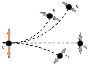
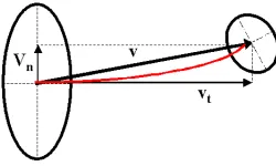
Figure 1: Illustration of tensor voting in 2-D. The voter is an oriented curve element V on a hori-zontal curve whose normal is represented by the orange arrow. The four receivers R1-R4 collect votes from V . (In practice, they would also cast votes to V and among themselves, but this is omitted here.) Each receiver is connected to V by a circular arc which is the simplest structure that can be inferred from two points, one of which is oriented. The gray votes at the receivers indicate the curve normal the receivers should have according to the voter.
a receiver is a circular arc, for which curvature is constant. Therefore, we connect the voter and receiver by a circular arc which is tangent at the voter and passes through the receiver and define the vote cast as the normal to this arc at the location of the receiver. The votes shown as gray arrows in Figure 1 represent the orientations the receivers would have according to the voter V . The mag-nitude of the votes decays with distance and curvature. It will be defined formally in Section 3.2. Voting from all possible types of voters, such as surface or curve elements in 3-D, can be derived from the fundamental case of a curve element voter in 2-D (Medioni et al., 2000). Tensor voting is based on strictly local computations in the neighborhoods of the inputs. The size of these neighbor-hoods is controlled by the only critical parameter in the framework: the scale of votingσ. The scale parameter is introduced in Eq. 3. By determining the size of the neighborhoods, scale regulates the amount of smoothness and provides a knob to the user for balancing fidelity to the data and noise reduction.
Regardless of the computational feasibility of an implementation, the same grouping principles apply to spaces with even higher dimensions. For instance, Tang et al. (2001) observed that pixel correspondences can be viewed as points in the 8-D space of free parameters of the fundamental matrix. Correct correspondences align to form a hyperplane in that space, while wrong correspon-dences are randomly distributed. By applying tensor voting in 8-D, Tang et al. were able to infer the dominant hyperplane and the desired parameters of the fundamental matrix. Storage and com-putation requirements, however, soon become prohibitively high as the dimensionality of the space increases. Even though the applicability of tensor voting as a manifold learning technique seems to have merit, the generalization of the implementation of Medioni et al. (2000) is not practical, mostly due to computational complexity and storage requirements in N dimensions. The bottleneck is the generation and storage of voting fields, the number of which is equal to the dimensionality of the space.
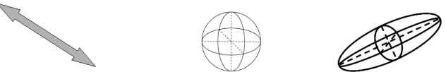
(a) Oriented or stick tensor (b) Unoriented or ball tensor (c) Generic tensor
Figure 2: Examples of tensors in 3-D. The tensor on the left has only one non-zero eigenvalue and encodes a preference for an orientation parallel to the eigenvector corresponding to that eigenvalue. The eigenvalues of the tensor in the middle are all equal, and thus the tensor does not encode a preference for a particular orientation. The tensor on the right is a generic 3-D tensor.
our work is a new formulation of the voting process that is practical for spaces of dimensionality up to a few hundreds. Efficiency is considerably higher than the preliminary version of this formulation presented in Mordohai and Medioni (2005), where we focused on dimensionality estimation.
3.1 Data Representation
The representation of a token (a generic data point) is a second order, symmetric, non-negative definite tensor, which is equivalent to an N×N matrix and an ellipsoid in an N-D space. All tensors
in this paper are second order, symmetric and non-negative definite, so any reference to a tensor automatically implies these properties. Three examples of tensors, in 3-D, can be seen in Figure 2. A tensor represents the structure of a manifold going through the point by encoding the normals to the manifold as eigenvectors of the tensor that correspond to non-zero eigenvalues, and the tangents as eigenvectors that correspond to zero eigenvalues. (Note that eigenvectors and vectors in general in this paper are column vectors.) For example, a point in an N-D hyperplane has one normal and
N−1 tangents, and thus is represented by a tensor with one non-zero eigenvalue associated with an eigenvector parallel to the hyperplane’s normal. The remaining N−1 eigenvalues are zero. A point belonging to a 2-D manifold in N-D is represented by two tangents and N−2 normals, and thus is represented by a tensor with two zero eigenvalues associated with the eigenvectors that span the tangent space of the manifold. The tensor also has N−2 non-zero, equal eigenvalues whose corresponding eigenvectors span the manifold’s normal space. Two special cases of tensors are: the
stick tensor that has only one non-zero eigenvalue and represents perfect certainty for a hyperplane
normal to the eigenvector that corresponds to the non-zero eigenvalue; and the ball tensor that has all eigenvalues equal and non-zero which represents perfect uncertainty in orientation, or, in other words, just the presence of an unoriented point.
The tensors can be formed by the summation of the direct products (~n~nT) of the eigenvectors that span the normal space of the manifold. The tensor at a point on a manifold of dimensionality
d, with~nibeing the unit vectors that span the normal space, can be computed as follows:
T = d
∑
i=1
An unoriented point can be represented by a ball tensor which contains all possible normals and is encoded as the N×N identity matrix. Any point on a manifold of known dimensionality and
orientation can be encoded in this representation by appropriately constructed tensors, according to Eq. 1.
On the other hand, given an N-D second order, symmetric, non-negative definite tensor, the type of structure encoded in it can be inferred by examining its eigensystem. Any such tensor can be decomposed as in the following equation:
T= N
∑
d=1
λdeˆdeˆTd =
= (λ1−λ2)eˆ1eˆT1 + (λ2−λ3)(eˆ1eˆT1+eˆ2eˆT2) +....+λN(eˆ1eˆT1+eˆ2eˆT2+...+eˆNeˆTN) =
N−1
∑
d=1
[(λd−λd+1) d
∑
k=1 ˆ
edeˆTd] +λN(eˆ1eˆT1+...+eˆNeˆTN)
(2)
whereλdare the eigenvalues in descending order of magnitude and ˆed are the corresponding eigen-vectors. The tensor simultaneously encodes all possible types of structure. The confidence, or
saliency in perceptual organization terms, of the type that has d normals is encoded in the
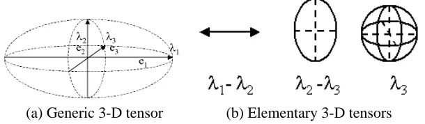
differ-enceλd−λd+1, or λN for the ball tensor. If only one of these eigenvalue differences is not zero, then the tensor encodes a single type of structure. Otherwise, more than one type can be present at the location of the tensor, each having a saliency value given by the appropriate difference between consecutive eigenvalues ofλN. An illustration of tensor decomposition in 3-D can be seen in Figure 3.
(a) Generic 3-D tensor (b) Elementary 3-D tensors
Figure 3: Tensor decomposition in 3-D. A generic tensor can be decomposed into the stick, plate and ball components that have a normal subspace of rank one, two and three respectively.
3.2 The Voting Process
After the inputs have been encoded with tensors, the information they contain is propagated to their neighbors via a voting operation. Given a tensor at A and a tensor at B, the vote the token at A (the
voter) casts to B (the receiver) has the orientation the receiver would have, if both the voter and
3.2.1 STICKVOTING
We first examine the case of a voter associated with a stick tensor, that is the normal space is a single vector in N-D. We claim that, in the absence of other information, the arc of the osculating circle (the circle that shares the same normal as a curve at the given point) at A that goes through B is the most likely smooth path between A and B, since it minimizes total curvature. The center of the circle is denoted by C in Figure 4(a). (For visualization purposes, the illustrations are for the 2-D and 3-D cases.) In case of straight continuation from A to B, the osculating circle degenerates to a straight line. Similar use of circular arcs can also be found in Parent and Zucker (1989), Saund (1992), Sarkar and Boyer (1994) and Yen and Finkel (1998). The vote is also a stick tensor and is generated as described in Section 3 according to the following equation:
Svote(s,θ,κ) = e−(s2+cκ
2
σ2 )
−sin(2θ) cos(2θ)
[−sin(2θ) cos(2θ)], (3)
θ = arcsin(~v Teˆ
1 k~vk),
s = θk~vk sin(θ),
κ = 2 sin(θ) k~vk .
In the above equation, s is the length of the arc between the voter and receiver, andκis its curvature (which can be computed from the radius AC of the osculating circle in Figure 4(a)),σis the scale of voting, and c is a constant, which controls the degree of decay with curvature. The constant c is a function of the scale and is optimized to make the extension of two orthogonal line segments to from a right angle equally likely to the completion of the contour with a rounded corner (Guy and Medioni, 1996). Its value is given by: c= −16log(0π.12)×(σ−1). The scaleσessentially controls
the range within which tokens can influence other tokens. It can also be viewed as a measure of smoothness that regulates the inevitable trade-off between over-smoothing and over-fitting. Small values preserve details better, but are more vulnerable to noise and over-fitting. Large values pro-duce smoother approximations that are more robust to noise. As shown in Section 7, the results are very stable with respect to the scale. Note thatσis the only free parameter in the framework.
The vote as defined above is on the plane defined by A, B and the normal at A. Regardless of the dimensionality of the space, stick vote generation always takes place in a 2-D subspace defined by the position of the voter and the receiver and the orientation of the voter. (This explains why Eq. 3 is defined in a 2-D space.) Stick vote computation is identical in any space between 2 and
N dimensions. After the vote has been computed, it has to be transformed to the N-D space and
aligned to the voter by a rotation and translation. For simplicity, we also use the notation:
Svote(A,B,~n) =S(s(A,B,~n),θ(A,B,~n),κ(A,B,~n)) (4)
to denote the stick vote from A to B with~n being the normal at A. s(A,B,~n),θ(A,B,~n)andκ(A,B,~n) are the resulting values of the parameters of Eq. 3 given A,B and~n.
continuation over curved alternatives. Moreover, no votes are cast if the receiver is at an angle larger than 45◦with respect to the tangent of the osculating circle at the voter. Similar restrictions on re-gions of influence also appear in Heitger and von der Heydt (1993), Yen and Finkel (1998) and Li (1998) to prevent high-curvature connections without support from the data. Votes corresponding to such connections would have been very weak regardless of the restriction since their magni-tude is attenuated due to curvature. The saliency decay function (Gaussian) of Eq. 3 has infinite support, but for practical purposes the field is truncated so that negligible votes do not have to be computed. For all experiments shown here, we limited voting neighborhoods to the extent in which the magnitude of a vote is more than 3% of the magnitude of the voter. Both truncation beyond 45◦ and truncation beyond a certain distance are not critical choices, but are made to eliminate the computation of insignificant votes.
3.2.2 N-D FORMULATION OFTENSORVOTING
We have shown that stick vote computation is identical up to a simple transformation from 2-D to N-D. Now we turn our attention to votes generated by voters that are not stick tensors. In the original formulation (Medioni et al., 2000) these votes can be computed by integrating the votes cast by a rotating stick tensor that spans the normal space of the voting tensor. Since the resulting integral has no closed form solution, the integration is approximated numerically by taking sample positions of the rotating stick tensor and adding the votes it generates at each point within the voting neighborhood. As a result, votes that cover the voting neighborhood are pre-computed and stored in voting fields. The advantage of this scheme is that all votes are generated based on the stick voting field. Its computational complexity, however, makes its application in high-dimensional spaces prohibitive. Voting fields are used as look-up tables to retrieve votes via interpolation between the pre-computed samples. For instance, a voting field in 10-D with k samples per axis, requires storage for k10 10×10 tensors, which need to be computed via numerical integration over 10 variables. Thus, the use of pre-computed voting fields becomes impractical as dimensionality grows. At the same time, the probability of using a pre-computed vote decreases.
Here, we present a simplified vote generation scheme that allows the direct computation of votes from arbitrary tensors in arbitrary dimensions. Storage requirements are limited to storing the tensors at each sample, since explicit voting fields are not used any more. The advantage of the novel vote generation scheme is that it does not require integration. As in the original formulation, the eigenstructure of the vote represents the normal and tangent spaces that the receiver would have, if the voter and receiver belong in the same smooth structure.
3.2.3 BALLVOTING
identity matrix). The resulting tensor is attenuated by the same Gaussian weight according to the distance between the voter and the receiver.
Bvote(s) =e−(
s2 σ2)
I
− ~v~v Tk~vT~vk
(5)
where~v is a unit vector parallel to the line connecting the voter and the receiver and
I
is the N-D identity matrix. In this case, s=|~v|and we omitθandκsince they do not affect the computation.Along the lines of Equation 4, we define a simpler notation:
Bvote(A,B) =Bvote(s(A,B)) (6)
where s(A,B) =|~v|.
3.2.4 VOTING BY ELEMENTARYTENSORS
To complete the description of vote generation, we need to describe the case of a tensor that has
d equal eigenvalues, where d is not equal to 1 or N. (An example of such a tensor would be a
curve element in 3-D, which has a rank-two normal subspace and a rank-one tangent subspace.) The description in this section also applies to ball and stick tensors, but we use the above direct computations, which are faster. Let~v be the vector connecting the voting and receiving points. It
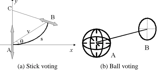
can be decomposed into~vt and~vn in the tangent and normal spaces of the voter respectively. The new vote generation process is based on the observation that curvature in Eq. 3 is not a factor when θis zero, or, in other words, if the voting stick is orthogonal to~vn. We can exploit this by defining a new basis for the normal space of the voter that includes~vn. The new basis is computed using the Gramm-Schmidt procedure. The vote is then constructed as the tensor addition of the votes cast by stick tensors parallel to the new basis vectors. Among those votes, only the one generated by the stick tensor parallel to~vnis not parallel to the normal space of the voter and curvature has to be considered. All other votes are a function of the length of~vt only. See Figure 5 for an illustration in 3-D. Analytically, the vote is computed as the summation of d stick votes cast by the new basis of the normal space. Let NSdenote the normal space of the voter and let~bi,i∈[1,d]be a basis for it with~b1being parallel to~vn. If Svote(A,B,~b)is the function that generates the stick vote from a
(a) Stick voting (b) Ball voting
Figure 5: Vote generation for generic tensors. The voter here is a tensor with a 2-D normal subspace in 3-D. The vector connecting the voter and receiver is decomposed into~vnand~vt that lie in the normal and tangent space of the voter. A new basis that includes~vn is defined for the normal space and each basis component casts a stick vote. Only the vote generated by the orientation parallel to~vnis not parallel to the normal space. Tensor addition of the stick votes produces the combined vote.
unit stick tensor at A parallel to~b to the receiver B, then the vote from a generic tensor with normal
space N is given by:
Vvote(A,B,Te,d) =Svote(A,B,~b1) +
∑
i∈[2,d]Svote(A,B,~bi). (7)
In the above equation, Te,ddenotes the elementary voting tensor with d equal non-zero eigenvalues. On the right-hand side, all the terms are pure stick tensors parallel to the voters, except the first one which is affected by the curvature of the path connecting the voter and receiver. Therefore, the computation of the last d−1 terms is equivalent to applying the Gaussian weight to the voting sticks and adding them at the position of the receiver. Only one vote requires a full computation of orientation and magnitude. This makes the proposed scheme computationally inexpensive.
3.2.5 THEVOTING PROCESS
During the voting process (Algorithm 1), each point casts a vote to all its neighbors within the voting neighborhood. If the voters are not pure elementary tensors, that is if more than one saliency value is non-zero, they are decomposed before voting according to Eq. 2. Then, each component votes separately and the vote is weighted byλd−λd+1, except the ball component whose vote is weighted byλN. Besides the voting tensor T, points also have a receiving tensor R that acts as vote accumulator. Votes are accumulated at each point by tensor addition, which is equivalent to matrix addition.
3.3 Vote Analysis
Vote analysis takes place after voting to determine the most likely type of structure and the orienta-tion at each point. There are N+1 types of structure in an N-D space ranging from 0-D points to
N-D hypervolumes.
Algorithm 1 The Voting Process 1. Initialization
Read M input points Piand initial conditions, if available. for all i∈[1,M]do
Initialize Tiaccording to initial conditions or set equal to the identity
I
. Compute Ti’s eigensystem(λ(di),eˆ(di)).Set vote accumulator Ri←0 end for
Initialize Approximate Nearest Neighbor (ANN) k-d tree (Arya et al., 1998) for fast neighbor retrieval.
2. Voting
for all i∈[1,M]do
for all Pjin Pi’s neighborhood do if λ1−λ2>0 then
Compute stick vote Svote(Pi,Pj,eˆ1(i))from Pito Pj according to Eq. 4. end if
if λN>0 then
Compute ball vote Bvote(Pi,Pj)from Pito Pjaccording to Eq. 6. end if
for d=2 to N−1 do
if λd−λd+1>0 then
Compute vote Vvote(Pi,Pj,T(ei,)d)according to Eq. 7. end if
end for
Add votes to Pj’s accumulator
Rj←Rj+ (λ1−λ2)Svote(Pi,Pj,eˆ1) + (λN)Bvote(Pi,Pj) +
∑
d∈[2,N−1]
(λd−λd+1)Vvote(Pi,Pj,T( i)
e,d)
end for end for
3. Vote Analysis for all i∈[1,M]do
Compute eigensystem of Ri (Eq. 2) to determine dimensionality and orientation. Ti←Ri
end for
dimensionality is N−d, and the manifold has d normals and N−d tangents. Moreover, the first d eigenvectors that correspond to the largest eigenvalues are the normals to the manifold, and the
small and no preferred structure type emerges. This happens because they are more isolated than inliers, thus they do not receive votes that consistently support any salient structure. Our past and current research has demonstrated that tensor voting is very robust against outliers.
This vote accumulation and analysis method does not optimize any explicit objective function, especially not a global one. Dimensionality emerges from the accumulation of votes, but it is not a equal to the average, nor the median, nor the majority of the dimensionalities of the voters. For instance, the accumulation of votes from elements of two or more intersecting curves in 2-D results in a rank-two normal space at the junction. If one restricts the analysis to the estimates of orientation, tensor voting can be viewed as a method for maximizing an objective at each point. The weighted (tensor) sum of all votes received is up to a constant equivalent to the weighted mean in the space of symmetric, non-negative definite, second-order tensors. This can be thought of as the tensor that maximizes the consensus among the incoming votes. In that sense, assuming dimensionality is provided by some other process, the estimated orientation at each point is the maximum likelihood estimate given the incoming votes. It should be pointed out here, that the sum is used for all subsequent computations, since the magnitude of the eigenvalues and the of the gaps between them are measures of saliency.
In all subsequent sections, the eigensystem of the accumulator tensor is used as the voter during subsequent processing steps described in the following sections.
Figure 6: 20,000 points sampled from the “Swiss Roll” data set in 3-D.
4. Dimensionality Estimation
In this section, we present experimental results in dimensionality estimation. According to Section 3.3, the intrinsic dimensionality at each point can be found as the maximum gap in the eigenvalues of the tensor after votes from its neighboring points have been collected. All inputs consist of unoriented points since no orientation information is provided and are encoded as ball tensors.
4.1 Swiss Roll
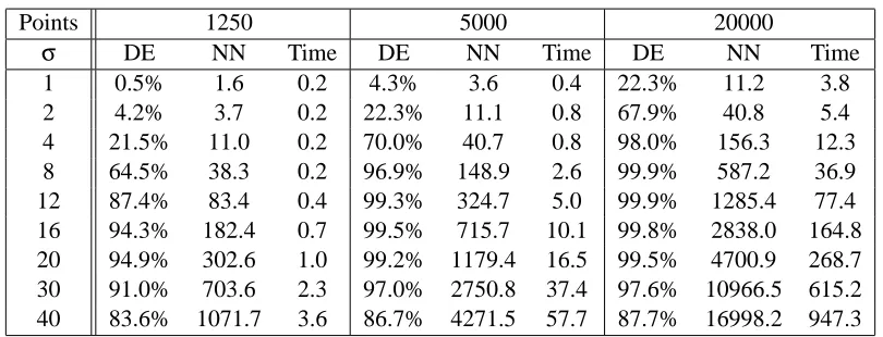
Points 1250 5000 20000
σ DE NN Time DE NN Time DE NN Time
1 0.5% 1.6 0.2 4.3% 3.6 0.4 22.3% 11.2 3.8
2 4.2% 3.7 0.2 22.3% 11.1 0.8 67.9% 40.8 5.4 4 21.5% 11.0 0.2 70.0% 40.7 0.8 98.0% 156.3 12.3 8 64.5% 38.3 0.2 96.9% 148.9 2.6 99.9% 587.2 36.9 12 87.4% 83.4 0.4 99.3% 324.7 5.0 99.9% 1285.4 77.4 16 94.3% 182.4 0.7 99.5% 715.7 10.1 99.8% 2838.0 164.8 20 94.9% 302.6 1.0 99.2% 1179.4 16.5 99.5% 4700.9 268.7 30 91.0% 703.6 2.3 97.0% 2750.8 37.4 97.6% 10966.5 615.2 40 83.6% 1071.7 3.6 86.7% 4271.5 57.7 87.7% 16998.2 947.3
Table 1: Rate of correct dimensionality estimation (DE), average number of neighbors per point and execution times (in seconds) as functions ofσand the number of samples for the “Swiss Roll” data set. All experiments have been repeated 10 times on random samplings of the Swiss Roll function. Note that the range of scales includes extreme values as evidenced by the very high and very low numbers of neighbors in several cases.
second column shows the average number of nearest neighbors included in the voting neighborhood of each point. The third column shows processing times of a single-threaded C++ implementation running on an Intell Pentium 4 processor at 2.50GHz. We have also repeated the experiment on 10 instances of 500 points from the Swiss Roll using the same values of the scale. Meaningful results are obtained forσ>8. The peak of correct dimensionality estimation is at 80.3% forσ=20.
A conclusion that can be drawn from Table 1 is that the accuracy is high and stable for a large range of values ofσ, as long as a few neighbors are included in each neighborhood. The majority of neighborhoods being empty is an indication of inappropriate scale selection. Performance degrades as scale increases and the neighborhoods become too large to capture the curvature of the manifold. This robustness to large variations in parameter selection are due to the weighting of the votes according to Eqs. 3, 5 and 7 and alleviates the need for extensive parameter tuning.
4.2 Structures with Varying Dimensionality
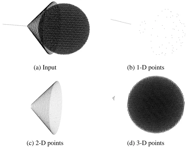
(a) Input (b) 1-D points
(c) 2-D points (d) 3-D points
Figure 7: Data of varying dimensionality in 4-D. (The first three dimensions of the input and the classified points are shown.) Note that the hyper-sphere is empty in 4-D, but appears as a full sphere when visualized in 3-D.
4.3 Data in High Dimensions
The data sets for this experiment were generated by sampling a few thousand points from a low-dimensional space (3- or 4-D) and mapping them to a medium low-dimensional space (14- to 16-D) using linear and quadratic functions. The generated points were then rotated and embedded in a 50- to 150-D space. Outliers drawn from a uniform distribution inside the bounding box of the data were added to the data set. The percentage of correct point-wise dimensionality estimates after tensor voting can be seen in Table 2.
Intrinsic Linear Quadratic Space Dimensionality Dimensionality Mappings Mappings Dimensions Estimation (%)
4 10 6 50 93.6
3 8 6 100 97.4
4 10 6 100 93.9
3 8 6 150 97.3
5. Manifold Learning
In this section we show quantitative results on estimating manifold orientation for various data sets.
Points 1250 5000 20000
σ Orientation Error Orientation Error Orientation Error
1 47.2 28.1 3.1
2 28.7 3.5 0.4
4 4.9 0.9 0.5
8 2.0 1.3 1.1
12 2.5 2.0 1.9
16 3.5 3.1 3.0
20 5.4 4.8 4.7
30 16.9 15.0 14.9
40 28.3 26.2 25.9
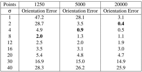
Table 3: Error (in degrees) in surface normal orientation estimation as a function of σ and the number of samples for the “Swiss Roll” data set. The error reported is the (unsigned) angle between the eigenvector corresponding to the largest eigenvalue of the estimated tensor at each point and the ground truth surface normal. See also Table 1 for processing times and the average number of points in each neighborhood.
5.1 Swiss Roll
We begin this section by completing the presentation of our experiments on the Swiss Roll data sets described in the previous section. Here we show the accuracy of normal estimation, regardless of whether the dimensionality was estimated correctly, for the experiments of Table 1. Table 3 is a complement to Table 1, which contains information on the average number of points in the voting neighborhoods and processing time that is not repeated here. The error reported is the (unsigned) angle between the eigenvector corresponding to the largest eigenvalue of the estimated tensor at each point and the ground truth surface normal. These results are over 10 different samplings for each number of points reported in the table.
For comparison, we also estimated the orientation at each point of the Swiss Roll using local PCA computed on the point’s k nearest neighbors. We performed an exhaustive search over k, but only report the best results here. As for tensor voting, orientation accuracy was measured on 10 instances of each data set. The lowest errors for 1,250, 5,000 and 20,000 points are 2.51◦, 1.16◦ and 0.56◦for values of k equal to 9, 10 and 13 respectively. These errors are approximately 20% larger than the lowest errors achieved by tensor voting, which are shown in bold in Table 3. It should be noted, that, unlike tensor voting, local PCA cannot be used to refine these estimates or take advantage of existing orientation estimates that may be available at the inputs.
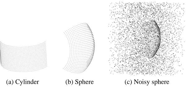
(a) Cylinder (b) Sphere (c) Noisy sphere
Figure 8: Data sets used in Sections 5 and 6.
bounds for the eigenvalues of square matrices. The authors show how noise and curvature affect the estimation of curve and surface normals under some assumptions about the distribution of the points. The conclusions are that for large neighborhood sizes, errors caused by curvature dominate, while for small neighborhood sizes, errors due to noise dominate. (There is no noise in the data for this experiment.)
5.2 Spherical and Cylindrical Sections
Here, we present quantitative results on simple data sets in 3-D for which ground truth can be analytically computed. In Section 6, we process the same data with state of the art manifold learning algorithms and compare their results against ours. The two data sets are a section of a cylinder and a section of a sphere shown in Figure 8. The cylindrical section spans 150◦ and consists of 1000 points. The spherical section spans 90◦×90◦and consists of 900 points. Both are approximately uniformly sampled. The points are represented by ball tensors, assuming no information about their orientation. In the first part of the experiment, we compute local dimensionality and normal orientation as a function of scale. The results are presented in Tables 4 and 5. The results show that if the scale is not too small, dimensionality estimation is very reliable. For all scales the orientation errors are below 0.4o.
σ Average Orientation Dimensionality Neighbors Error(◦) Estimation (%)
10 5 0.06 4
20 9 0.07 90
30 9 0.08 90
40 12 0.09 90
50 20 0.10 100
60 20 0.11 100
70 23 0.12 100
80 25 0.12 100
90 30 0.13 100
100 34 0.14 100
Table 4: Results on the cylinder data set. Shown in the first column isσ, in the second is the average number of neighbors that cast votes to each point, in the third the average error in degrees of the estimated normals, and in the fourth the accuracy of dimensionality estimation.
σ Average Orientation Dimensionality Neighbors Error(◦) Estimation (%)
10 5 0.20 44
20 9 0.23 65
30 11 0.24 93
40 20 0.26 94
50 21 0.27 94
60 23 0.29 94
70 26 0.31 94
80 32 0.34 94
90 36 0.36 94
100 39 0.38 97
Table 5: Results on the sphere data set. The columns are the same as in Table 4.
due to the structure imposed to them by the mapping, which makes the outliers less random, and due to the increase in their density in the low-dimensional space compared to that in the original high-dimensional space.
5.3 Data with Non-uniform Density
We also conducted two experiments on functions proposed in Wang et al. (2005). The key difficulty with these functions is the non-uniform density of the data. In the first example we attempt to estimate the tangent at the samples of:
Outliers 900 3000 5000 σ 10 20 30 40 50 60 70 80 90 100 OE DE 1.15 44 0.93 65 0.88 92 0.88 93 0.90 93 0.93 94 0.97 94 1.00 94 1.04 95 1.07 97 OE DE 3.68 41 2.95 52 2.63 88 2.49 90 2.41 92 2.38 93 2.38 93 2.38 94 2.38 95 2.39 95 OE DE 6.04 39 4.73 59 4.15 85 3.85 88 3.63 91 3.50 93 3.43 93 3.38 94 3.34 94 3.31 95
Table 6: Results on the sphere data set contaminated by noise. OE: error in normal estimation in degrees, DE: percentage of correct dimensionality estimation.
(a) Samples from Eq. 8 (b) Samples from Eq. 9
Figure 9: Input data for the two experiments proposed by Wang et al. (2005).
where the distance between consecutive samples is far from uniform. See Figure 9(a) for the inputs and the second column of Table 7 for quantitative results on tangent estimation for 152 points as a function of scale.
In the second example, which is also taken from Wang et al. (2005), points are uniformly sam-pled on the t-axis from the [-6, 6] interval. The output is produced by the following function:
xi= [ti 10e−t
2
i]. (9)
σ Eq. 8 Eq. 9 Eq. 9 152 points 180 points 360 points
10 0.60 4.52 2.45
20 0.32 3.37 1.89
30 0.36 2.92 1.61
40 0.40 2.68 1.43
50 0.44 2.48 1.22
60 0.48 2.48 1.08
70 0.51 2.18 0.95
80 0.54 2.18 0.83
90 0.58 2.02 0.68
100 0.61 2.03 0.57
Table 7: Error in degrees for tangent estimation for the functions of Eq. 8 and Eq. 9.
6. Geodesic Distances and Nonlinear Interpolation
In this section, we present an algorithm that can interpolate, and thus produce new points, on the manifold and is also able to evaluate geodesic distances between points. Both of these capabilities are useful tools for many applications. The key concept is that the intrinsic distance between any two points on a manifold can be approximated by taking small steps on the manifold, collecting votes, estimating the local tangent space and advancing on it until the destination is reached. Such processes have been reported in Mordohai (2005), Doll´ar et al. (2007a) and Doll´ar et al. (2007b).
Processing begins by learning the manifold structure, as in the previous section, usually starting from unoriented points that are represented by ball tensors. Then, we select a starting point that has to be on the manifold and a target point or a desired direction from the starting point. At each step, we can project the desired direction on the tangent space of the current point and create a new point at a small distance. The tangent space of the new point is computed by collecting votes from the neighboring points, as in regular tensor voting. Note that the tensors used here are no longer balls, but the ones resulting from the previous pass of tensor voting, according to Algorithm 1, step 3. The desired direction is then projected on the tangent space of the new point and so forth until the destination is reached. The process is illustrated in Figure 10, where we start from point A and wish to reach B. We project~t, the vector from A to B, on the estimated tangent space of A and obtain its
projection~p. Then, we take a small step along~p to point A1, on which we collect votes to obtain an estimate of its tangent space. The desired direction is then projected on the tangent space of each new point until the destination is reached withinε. The geodesic distance between A and B is approximated by measuring the length of the path. In the process, we have also generated a number of new points on the manifold, which may be a desirable by-product for some applications.
Figure 10: Nonlinear interpolation on the tangent space of a manifold.
converges to the destination and the geodesic distance is approximated accurately using a small step size. A second failure mode of the simple algorithm is for cases where the desired direction may vanish. This may occur in a manifold such as the “Swiss Roll” (Figure 6) if the destination lies on the normal space of the current point. Adding memory or inertia to the system when the desired direction vanishes, effectively addresses this situation. It should be noted that our algorithm does not handle holes and boundaries properly at its current stage of development.
6.1 Comparison with State-of-the-Art algorithms
The first experiment on manifold distance estimation is a quantitative evaluation against some of the most widely used algorithms of the literature. For the results reported in Table 8, we learn the local structure of the cylinder and sphere manifolds of the previous section using tensor voting. We also compute embeddings using LLE (Roweis and Saul, 2000), Isomap (Tenenbaum et al., 2000), Laplacian eigenmaps (Belkin and Niyogi, 2003), HLLE (Donoho and Grimes, 2003) and SDE (Weinberger and Saul, 2004). Matlab implementations for these methods can be downloaded from the following internet locations.
• LLE fromhttp://www.cs.toronto.edu/˜roweis/lle/code.html
• Isomap fromhttp://isomap.stanford.edu/
• Laplacian Eigenmaps fromhttp://people.cs.uchicago.edu/˜misha/ManifoldLearning/ index.html
• HLLE fromhttp://basis.stanford.edu/HLLEand
• SDE fromhttp://www.seas.upenn.edu/˜kilianw/sde/download.htm.
We are grateful to the authors for making the code for their methods available to the community. We have also made our software publicly available at:
http://iris.usc.edu/˜medioni/download/download.htm.
space using tensor voting and in the embedding space using the other five methods. The estimated distances are compared to the ground truth: r∆θfor the sphere andp(r∆θ)2+ (∆z)2for the cylin-der. Among the above approaches, only Isomap and SDE produce isometric embeddings, and only Isomap preserves the absolute distances between the input and the embedding space. To make the evaluation fair, we compute a uniform scale that minimizes the error between the computed dis-tances and the ground truth for all methods, except Isomap for which it is not necessary. Thus, perfect distance ratios would be awarded a perfect rating in the evaluation, even if the absolute magnitudes of the distances are meaningless in the embedding space. For all the algorithms, we tried a wide range for the number of neighbors, K. In some cases, we were not able to produce good embeddings of the data for any value of K. This occurred more frequently for the cylinder, probably due to its data density not being perfectly uniform. Errors above 20% indicate very poor performance, which is also confirmed by visual inspection of the embeddings.
Even though among the other approaches only Isomap and SDE produce isometric embeddings, while the rest produce embeddings that only preserve local structure, we think that the evaluation of the quality of manifold learning based on the computation of pairwise distances is a fair measure for the performance of all algorithms, since high quality manifold learning should minimize distortions. The distances on which we evaluate the different algorithms are both large and small, with the latter measuring the presence of local distortions. Quantitative results, in the form of the average absolute difference between the estimated and the ground truth distances as a percentage of the latter, are presented in Tables 8-10, along with the parameter that achieves the best performance for each method. In the case of tensor voting, the same scale was used for both learning the manifold and computing distances.
We also apply our method in the presence of 900, 3000 and 5000 outliers, while the inliers for the sphere and the cylinder data sets are 900 and 1000 respectively. The outliers are generated according to a uniform distribution. The error rates using tensor voting for the sphere are 0.39%, 0.47% and 0.53% respectively. The rates for the cylinder are 0.77%, 1.17% and 1.22%. Compared with the noise free case, these results demonstrate that our approach degrades slowly in the presence of outliers. The best performance achieved by any other method is 3.54% on the sphere data set with 900 outliers by Isomap. Complete results are shown in Table 9. In many cases, we were unable to achieve useful embeddings for data sets with outliers. We were not able to perform this experiment
Data Set Sphere Cylinder
K Err(%) K Err(%)
LLE 18 5.08 6 26.52
Isomap 6 1.98 30 0.35
Laplacian Eigenmaps 16 11.03 10 29.36
HLLE 12 3.89 40 26.81
SDE 2 5.14 6 25.57
TV (σ) 60 0.34 50 0.62
Data Set Sphere Cylinder
900 outliers 900 outliers
K Err(%) K Err(%)
LLE 40 60.74 6 15.40
Isomap 18 3.54 14 11.41
Laplacian Eigenmaps 6 13.97 14 27.98
HLLE 30 8.73 30 23.67
SDE N/A N/A
TV (σ) 70 0.39 100 0.77
Table 9: Error rates in distance measurement between pairs of points on the manifolds under outlier corruption. The best result of each method is reported along with the number of neighbors used for the embedding (K), or the scale σin the case of tensor voting (TV). Note that HLLE fails to compute an embedding for small values of K, while SDE fails at both examples for all choices of K.
Data Set σ Error rate
Sphere (3000 outliers) 80 0.47 Sphere (5000 outliers) 100 0.53 Cylinder (3000 outliers) 100 1.17 Cylinder (5000 outliers) 100 1.22
Table 10: Error rates for our approach for the experiment of Section 6.1 in the presence of 3000 and 5000 outliers.
in the presence of more than 3000 outliers with any graph-based method, probably because the graph structure is severely corrupted by the outliers.
6.2 Data Sets with Varying Dimensionality and Intersections
For the final experiment of this section, we create synthetic data in 3-D that were embedded in higher dimensions. The first data set consists of a line and a cone. The points are embedded in 50-D by three orthonormal 50-D vectors and initialized as ball tensors. Tensor voting is performed in the 50-D space and a path from point A on the line to point B on the cone is interpolated as in the previous experiment, making sure that it belongs to the local tangent space, which changes dimensionality from one to two. The data is re-projected back to 3-D for visualization in Figure 11(a).
(a) Line and cone (b) S and plane
Figure 11: Nonlinear interpolation in 50-D with varying dimensionality (a) and 30-D with inter-secting manifolds under noise corruption (b).
points in 30-D is 2 min. and 40 sec. on a Pentium 4 at 2.8GHz using voting neighborhoods that included an average of 44 points.
7. Generation of Unobserved Samples and Nonparametric Function Approximation
In this section, we build upon the results of the previous section to address function approximation. A common practice is to treat functions with multiple outputs as multiple single-output functions. We adopt this scheme here, even though nothing prohibits us from directly approximating multiple-input multiple-output functions. We assume that observations in N-D that include values for the input and output variables are available for training. The difference with the examples of the pre-vious sections is that the queries are given as input vectors with unknown output values, and thus are of lower dimensionality than the voting space. The required module to convert this problem to that of Section 6 is one that can find a point on the manifold that corresponds to an input similar to the query. Then, in order to predict the output y of the function for an unknown input~x, under the
assumption of local smoothness, we move on the manifold formed by the training samples until we reach the point corresponding to the given input coordinates. To ensure that we always remain on the manifold, we need to start from a point on it and proceed as in the previous section.
One way to find a suitable starting point is to find the nearest neighbor of~x in the input space,
Figure 12: Interpolation to obtain output value for unknown input point Ai. Bi is the nearest neigh-bor in the input space and corresponds to B in the joint input-output space. We can march from B on the manifold to arrive at the desired solution A that projects on Ai in the input space.
outputs, or use other information, such as the previous state of the system, to pursue only one of the alternatives. One could find multiple nearest neighbors, run the proposed algorithm starting from each of them and produce a multi-valued answer with a probability associated with each potential output value.
Figure 12 provides a simple illustration. We begin with a point Ai in the input space. We proceed by finding its nearest neighbor among the projections of the training data on the input space
Bi. (Even if Biis not the nearest neighbor the scheme still works but possibly requires more steps.) The sample B in the input-output space that corresponds to Biis the starting point on the manifold. The desired direction is the projection of the AiBi vector on the tangent space of B. Now, we are in the case described in Section 6, where the starting point and the desired direction are known. Processing stops when the input coordinates of the point on the path from B are withinεof Ai. The corresponding point A in the input-output space is the desired interpolated sample.
As in all the experiments presented in this paper, the input points are encoded as ball tensors, since we assume that we have no knowledge of their orientation. We first attempt to approximate the following function, proposed by Schaal and Atkeson (1998):
y=max{e−10x21 e−50x22 1.25e−5(x21+x22)}. (10)
1681 samples of y are generated by uniformly sampling the[−1,1]×[−1,1]square. We perform four experiments with increasing degree of difficulty. In all cases, after voting on the given inputs, we generate new samples by interpolating between the input points. The four configurations and noise conditions were:
• In the first experiment, we performed all operations with noise free data in 3-D.
• For the second experiment, we added 8405 outliers (five times more than the inliers) drawn from a uniform distribution in a 2×2×2 cube containing the data.
(a) Noise free inputs (b) Inputs with outliers
(c) Interpolated points with (d) Interpolated points with outliers and perturbation outliers and perturbation in 60-D
Figure 13: Inputs and interpolated points for Eq. 10. The top row shows the noise-free inputs and the noisy input set where only 20% of the points are inliers. The bottom row shows the points generated in 3-D and 60-D respectively. In both cases the inputs were contami-nated with outliers and Gaussian noise.
• Finally, we embedded the perturbed data (and the outliers) in a 60-D space, before voting and nonlinear interpolation.