Theoretical Analysis of Bayesian Matrix Factorization

Theoretical Analysis of Bayesian Matrix Factorization

Shinichi Nakajima [email protected]

Optical Research Laboratory Nikon Corporation

Tokyo 140-8601, Japan

Masashi Sugiyama [email protected]

Department of Computer Science Tokyo Institute of Technology Tokyo 152-8552, Japan

Editor: Inderjit Dhillon

Abstract

Recently, variational Bayesian (VB) techniques have been applied to probabilistic matrix factor-ization and shown to perform very well in experiments. In this paper, we theoretically elucidate properties of the VB matrix factorization (VBMF) method. Through finite-sample analysis of the VBMF estimator, we show that two types of shrinkage factors exist in the VBMF estimator: the positive-part James-Stein (PJS) shrinkage and the trace-norm shrinkage, both acting on each sin-gular component separately for producing low-rank solutions. The trace-norm shrinkage is simply induced by non-flat prior information, similarly to the maximum a posteriori (MAP) approach. Thus, no trace-norm shrinkage remains when priors are non-informative. On the other hand, we show a counter-intuitive fact that the PJS shrinkage factor is kept activated even with flat priors. This is shown to be induced by the non-identifiability of the matrix factorization model, that is, the mapping between the target matrix and factorized matrices is not one-to-one. We call this model-induced regularization. We further extend our analysis to empirical Bayes scenarios where hyperparameters are also learned based on the VB free energy. Throughout the paper, we assume no missing entry in the observed matrix, and therefore collaborative filtering is out of scope.

Keywords: matrix factorization, variational Bayes, empirical Bayes, positive-part James-Stein shrinkage, non-identifiable model, model-induced regularization

1. Introduction

The goal of matrix factorization (MF) is to find a low-rank expression of a target matrix. MF can be used for learning linear relation between vectors such as reduced rank regression (Baldi and Hornik, 1995; Reinsel and Velu, 1998), canonical correlation analysis (Hotelling, 1936; Anderson, 1984), partial least-squares (Wold, 1966; Worsley et al., 1997; Rosipal and Kr¨amer, 2006), and

multi-task learning (Chapelle and Harchaoui, 2005; Yu et al., 2005). More recently, MF is applied

to collaborative filtering for imputing missing entries of a target matrix, for example, in the context of recommender systems (Konstan et al., 1997; Funk, 2006) and microarray data analysis (Baldi and Brunak, 1998). For these reasons, MF has attracted considerable attention these days.

1.1 MF Methods

Srebro and Jaakkola (2003) proposed the weighted low-rank approximation method, which is based on the expectation-maximization (EM) algorithm: a matrix is fitted to the data without a rank con-straint in the E-step and it is projected back to the set of low-rank matrices by singular value

de-composition (SVD) in the M-step. Since the optimization problem of the weighted low-rank

ap-proximation method involves a low-rank constraint, it is non-convex and thus only a local optimal solution may be obtained. Furthermore, SVD of the target matrix needs to be carried out in each iteration, which may be computationally intractable for large-scale data.

Funk (2006) proposed the regularized SVD method that minimizes a goodness-of-fit term com-bined with the Frobenius-norm penalty under a low-rank constraint by gradient descent (see also Paterek, 2007). The regularized SVD method could be computationally more efficient than the weighted low-rank approximation method in the context of collaborative filtering since only ob-served entries are referred to in each gradient iteration.

Srebro et al. (2005) proposed to use the trace-norm penalty instead of the Frobenius-norm penalty, so that a low-rank solution can be obtained without having an explicit low-rank constraint. Thanks to the convexity of the trace-norm, a semi-definite programming formulation can be ob-tained when the hinge-loss (Sch¨olkopf and Smola, 2002) is used. See also Rennie and Srebro (2005) for a computationally efficient variant using a gradient-based optimization method with smooth ap-proximation.

Salakhutdinov and Mnih (2008) proposed a Bayesian maximum a posteriori (MAP) method based on the Gaussian noise model and Gaussian priors on the decomposed matrices. This method actually corresponds to minimizing the squared-loss with the trace-norm penalty (Srebro et al., 2005).

Recently, the variational Bayesian (VB) approach (Attias, 1999) has been applied to MF (Lim and Teh, 2007; Raiko et al., 2007), which we refer to as VBMF. The VBMF method was shown to perform very well in experiments. However, its good performance was not completely understood beyond its experimental success. The purpose of this paper is to provide new insight into Bayesian MF.

1.2 MF Models and Non-identifiability

The MF models can be regarded as re-parameterization of the target matrix using low-rank matrices. This kind of re-parameterization often significantly changes the statistical behavior of the estimator (Gelman, 2004). Indeed, MF models possess a special structure called non-identifiability (Watan-abe, 2009), meaning that the mapping between the target matrix and the factorized matrices is not one-to-one .

Previous theoretical studies on non-identifiable models investigated the behavior of multi-layer

pereptrons, Gaussian mixture models, and hidden Markov models. It was shown that when such

reduced rank regression models, theoretical properties of VB have also been investigated (Watanabe and Watanabe, 2006; Nakajima and Watanabe, 2007).

1.3 Our Contribution

In this paper, following the line of Nakajima and Watanabe (2007) which investigated asymptotic behavior of VBMF estimators and the generalization error, we provide a more precise analysis of VB estimators. More specifically, we derive non-asymptotic bounds of the VBMF estimator. The obtained solution can be seen as a re-weighted singular value decomposition, and the weights in-clude a factor induced by the Bayesian inference procedure, in the same way as automatic relevance

determination (Neal, 1996; Wipf and Nagarajan, 2008).

We show that VBMF consists of two shrinkage factors, the positive-part James-Stein (PJS) shrinkage (James and Stein, 1961; Efron and Morris, 1973) and the trace-norm shrinkage (Srebro et al., 2005), operating on each singular component separately for producing low-rank solutions.

The trace-norm shrinkage is simply induced by non-flat prior information, as in the MAP ap-proach (Salakhutdinov and Mnih, 2008). Thus, no trace-norm shrinkage remains when priors are non-informative. On the other hand, we show a counter-intuitive fact that the PJS shrinkage factor is still kept activated even with uniform priors. This allows the VBMF method to avoid overfitting (or in some cases, this may cause underfitting) even when non-informative priors are provided. We call this regularization effect model-induced regularization since it is caused by the structure of the model likelihood function.

We further extend the above analysis to empirical VBMF (EVBMF) scenarios, where hyperpa-rameters in prior distributions are also learned based on the VB free energy. We derive bounds of the EVBMF estimator, and show that the effect of PJS shrinkage is at least doubled compared with the uniform prior cases.

Finally, we note that our analysis relies on the following three assumptions: First, we assume that the given matrix is fully observed, and no missing entry exists. This means that missing entry prediction is out of scope of our theory. Second, we require the noise to be independent Gaussian noise and the priors to be isotropic Gaussian. Third, we assume the column-wise independence on the VB posterior, which is different from the standard VB assumption that only the matrix-wise independence is required.

1.4 Organization

The rest of this paper is organized as follows. In Section 2, we formulate the MF problem and review its Bayesian approaches including FB, MAP, VB methods, and their empirical variants. In Section 3, we analyze the behavior of MAPMF, VBMF, and their empirical variants, and elucidate the regularization mechanism. In Section 4, we illustrate the characteristic behavior of MF solutions through simple numerical experiments, highlighting the influence of non-identifiability of the MF models. Finally, we conclude in Section 5. A brief review of the James-Stein shrinkage estimator and all the technical details are provided in Appendix.

2. Bayesian Approaches to Matrix Factorization

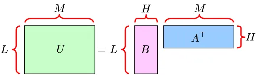
Figure 1: Matrix factorization model.

2.1 Formulation

The goal of the MF problem is to estimate a target matrix U(_∈RL×M_{)from its observation}

V_∈RL×M_.

Throughout the paper, we assume that

L_≤M.

If L>M, we may simply re-define the transpose U⊤as U so that L_≤M holds. Thus this does not

impose any restriction.

A key assumption of MF is that U is a low-rank matrix. Let H (_≤L) be the rank of U . Then the

matrix U can be decomposed into the product of A_∈RM×H_{and B∈R}L×H_{as follows (see Figure 1):}

U=BA⊤.

With appropriate pre-whitening (Hyv¨arinen et al., 2001), reduced rank regression (Baldi and Hornik, 1995; Reinsel and Velu, 1998), canonical correlation analysis (Hotelling, 1936; Anderson, 1984), partial least-squares (Wold, 1966; Worsley et al., 1997; Rosipal and Kr¨amer, 2006), and

multi-task learning (Chapelle and Harchaoui, 2005; Yu et al., 2005) can be seen as special cases of

the MF problem. Collaborative filtering (Konstan et al., 1997; Baldi and Brunak, 1998; Funk, 2006) and image processing (Lee and Seung, 1999) would be popular applications of MF. Note that, some of these applications such as collaborative filtering and multi-task learning with unshared input sets are out of scope of our theory, since they require missing entry prediction.

Assume that the observed matrix V is subject to the following additive-noise model:

V =U+

E

where

E

_E

Gaussian distribution with mean zero and varianceσ2. Then, the likelihood p(V_|A,B)is given by

p(V_|A,B)∝exp

−_2σ1₂kV₋BA⊤_k2_Fro

, (1)

2.2 Full-Bayesian Matrix Factorization (FBMF) and Its Empirical Variant (EFBMF)

We use the Gaussian priors on the parameters A and B:

φ(U) =φA(A)φB(B),

where

φA(A)∝exp −

H

∑

h=1

kahk2 2c2

ah !

=exp −tr(AC−

1 A A⊤) 2

!

, (2)

φB(B)∝exp −

H

∑

h=1

kbhk2 2c2_b

h !

=exp

−tr(BC−

1 B B⊤) 2

. (3)

Here,ahandbhare the h-th column vectors of A and B, respectively, that is,

A= (a1, . . . ,aH),

B= (b1, . . . ,bH).

c2_ah and c2_b

h are hyperparameters corresponding to the prior variances of those vectors. Without loss

of generality, we assume that the product cahcbh is non-increasing with respect to h. We also denote

them as covariance matrices:

CA=diag(c2a1, . . . ,c 2 aH), CB=diag(c2b1, . . . ,c

2 bH),

where diag(c)denotes the diagonal matrix with its entries specified by vectorc. tr(_·)denotes the trace of a matrix.

With the Bayes theorem and the definition of marginal distributions, the Bayes posterior p(A,B_|V) can be written as

p(A,B|V) = p(A,B,V)

p(V) =

p(V_|A,B)φA(A)φB(B)

hp(V_|A,B)_iφA(A)φB(B)

, (4)

where_h·ip denotes the expectation over p. The full-Bayesian (FB) solution is given by the Bayes

posterior mean:

b

UFB=_hBA⊤_ip(A,B|V). (5)

We call this method FBMF.

The hyperparameters cah and cbh may be determined so that the Bayes free energy F(V) is

minimized.

F(V) =₋log p(V)

=₋log_hp(V_|A,B)_iφA(A)φB(B). (6)

We call this method the empirical full-Bayesian MF (EFBMF). The Bayes free energy is also referred to as the marginal log-likelihood (MacKay, 2003), the evidence (MacKay, 1992) or the

2.3 Maximum A Posteriori Matrix Factorization (MAPMF) and Its Empirical Variant (EMAPMF)

When computing the Bayes posterior (4), the expectation in the denominator of Equation (4) is often intractable due to high dimensionality of the parameters A and B. More importantly, computing the posterior mean (5) is also intractable. A simple approach to mitigating this problem is to use the

maximum a posteriori (MAP) approximation, which we refer to as MAPMF. The MAP solution b

UMAPis given by

b

UMAP=BbMAP(AbMAP)⊤,

where

(AbMAP,BbMAP) =argmax A,B

p(A,B_|V).

In the MAP framework, one may determine the hyperparameters cah and cbh so that the Bayes

posterior p(A,B_|V) is maximized (equivalently, the negative log posterior is minimized). We call this method empirical MAPMF (EMAPMF). Note that EMAPMF does not work properly, as ex-plained in Section 3.3.

2.4 Variational Bayesian Matrix Factorization (VBMF) and Its Empirical Variant (EVBMF)

Another approach to avoiding computational intractability of the FB method is to use the variational

Bayes (VB) approximation (Attias, 1999; Bishop, 2006). Here, we review the VB-based MF method

(Lim and Teh, 2007; Raiko et al., 2007).

Let r(A,B_|V) be a trial distribution for A and B, and we define the following functional FVB called the VB free energy with respect to r(A,B_|V):

FVB(r|V) =

logr(A,B|V)

p(V,A,B)

r(A,B|V)

. (7)

Using p(V,A,B) =p(A,B_|V)p(V), we can decompose Equation (7) into two terms:

FVB(r|V) =

logr(A,B|V)

p(A,B_|V)

r(A,B|V)

+F(V), (8)

where F(V)is the Bayes free energy defined by Equation (6). The first term in Equation (8) is the

Kullback-Leibler divergence (Kullback and Leibler, 1951) from r(A,B_|V) to the Bayes posterior

p(A,B_|V). This is non-negative and vanishes if and only if the two distributions agree with each other. Therefore, the VB free energy FVB(r_|V)is lower-bounded by the Bayes free energy F(V):

FVB(r|V)≥F(V),

where the equality is satisfied if and only if r(A,B_|V)agrees with p(A,B_|V).

The VB approach minimizes the VB free energy FVB(r_|V)with respect to the trial distribution

r(A,B_|V), by restricting the search space of r(A,B_|V)so that the minimization is computationally tractable. Typically, dissolution of probabilistic dependency between entangled parameters (A and

B in the case of MF) makes the calculation feasible:

Then, the VB free energy (7) is written as

FVB(r|V) =

log rA(A|V)rB(B|V)

p(V_|A,B)φA(A)φB(B)

rA(A|V)rB(B|V)

. (10)

The resulting distribution is called the VB posterior. The VB solutionUbVB is given by the VB

posterior mean:

b

UVB=_hBA⊤_ir(A,B_|V). (11)

We call this method VBMF.

Applying the variational method to the VB free energy shows that the VB posterior satisfies the following conditions:

rA(A|V)∝ φA(A)exp hlog p(V|A,B)irB(B|V)

, (12)

rB(B|V)∝ φB(B)exp hlog p(V|A,B)irA(A|V)

. (13)

Recall that we are using the Gaussian priors (2) and (3). Also, Equation (1) implies that the log-likelihood log p(V_|A,B) is a quadratic function of A when B is fixed, and vice versa. Then the conditions (12) and (13) imply that the VB posteriors rA(A|V) and rB(B|V) are also Gaussian. This enables one to derive a computationally efficient algorithm called the iterated conditional

modes (Besag, 1986; Bishop, 2006), where the mean and the covariance of the parameters A and B are iteratively updated using Equations (12) and (13) (Lim and Teh, 2007; Raiko et al., 2007).

This amounts to alternating between minimizing the free energy (10) with respect to rA(A_|V)and

rB(B|V).

As in Raiko et al. (2007), we assume in our theoretical analysis that the trial distribution

r(A,B_|V)can be further factorized as

r(A,B_|V) =

H

∏

h=1

rah(ah|V)rbh(bh|V). (14)

Then the update rules (12) and (13) are simplified as

rah(ah|V)∝ φah(ah)exp

hlog p(V_|A,B)_ir_\ah(A\ah,B|V)

, (15)

rbh(bh|V)∝ φbh(bh)exp

hlog p(V_|A,B)_ir

\bh(A,B\bh|V)

, (16)

where r_\ahand r\bh denote the VB posterior of the parameters A and B exceptahandbh, respectively. The VB free energy also allows us to determine the hyperparameters c2_ah and c2_b

h in a

computa-tionally tractable way. That is, instead of the Bayes free energy F(V), the VB free energy FVB(r|V) is minimized with respect to c2_ah and c2_b

h. We call this method empirical VBMF (EVBMF).

3. Analysis of Bayesian MF Methods

3.1 MAPMF

The MAP estimator(AbMAP,BbMAP) is the maximizer of the Bayes posterior. In our model (1), (2), and (3), the negative log of the Bayes posterior is expressed as

−log p(A,B|V) =LM logσ 2

2 +

1 2

H

∑

h=1

M log c2_ah+L log c2_bh+kahk 2

c2 ah

+kbhk 2

c2 bh

!

+ 1 2σ2

V−

H

∑

h=1

bha⊤h

2 Fro

+Const. (17)

Differentiating Equation (17) with respect to A and B and setting the derivatives to zero, we have the following conditions:

ah=

kbhk2+ σ2

c2 ah

−1

V−

∑

h′_6=h

bh′a⊤_h′

!⊤

bh, (18)

bh= kahk2+

σ2

c2_b h

!−1

V₋

∑

h′_6=h

bh′a⊤_h′

!

ah. (19)

One may search a local solution (i.e., a local minimum of the negative log posterior (17)) by iterating Equations (18) and (19). However, as shown below, the optimal solution can be obtained analytically in the current setup.

When the hyperparameters are homogeneous, that is,_{cahcbh=c;∀h=1, . . . ,H}, a closed-form

expression of the MAP estimator can be immediately obtained by combining the results given in Srebro et al. (2005) and Cai et al. (2010). The following theorem is its slight extension that covers heterogeneous cases (its proof is given in Appendix B):

Theorem 1 Letγh(≥0)be the h-th largest singular value of V . Letωah andωbh be the associated right and left singular vectors:

V =

L

∑

h=1

γhωbhωa⊤h. (20)

The MAP estimatorUbMAP_{is given by}

b

UMAP=

H

∑

h=1

bγMAP

h ωbhωa⊤h,

where

bγMAP

h =max

0,γh− σ2

cahcbh

. (21)

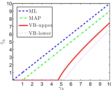
The theorem implies that the MAP solution cuts off the singular values less than σ2_/(c ahcbh);

otherwise it reduces the singular values byσ2/(cahcbh)(see Figure 2). This shrinkage effect allows

1 2 3 4 5 6 7 8 9 10 1

2 3 4 5 6 7 8 9 10

γh

b

γh

ML MAP VB-upp er VB-lower

Figure 2: Shrinkage of the ML estimator (22), the MAP estimator (21), and the VB estimator (28) whenσ2=0.1, cahcbh =0.1, L=100, and M=200.

Similarly to Theorem 1, we can show that the maximum likelihood (ML) estimator is given by

b

UML=

H

∑

h=1

bγML

h ωbhωa⊤h,

where

bγML

h =γhfor all h. (22)

Thus the ML solution is reduced to V when H=L (see Figure 2):

b

UML=

L

∑

h=1

bγML

h ωbhω⊤ah=V.

A parametric model is said to be identifiable if the mapping between parameters and functions is one-to-one; otherwise the model is said to be non-identifiable (Watanabe, 2001). Since the

decom-position U=BA⊤is redundant, the MF model is non-identifiable (Nakajima and Watanabe, 2007).

For identifiable models, the MAP estimator with the uniform prior is reduced to the ML estimator (Bishop, 2006). On the other hand, in the MF model, a single point in the space of U corresponds to a set of points in the joint space of A and B. For this reason, the uniform priors on A and B do not produce the uniform prior on U . Nevertheless, Equations (21) and (22) imply that MAP is reduced to ML when the priors on A and B are uniform (i.e., cah,cbh →∞).

More precisely, Equations (21) and (22) show that the product cahcbh→∞is sufficient for MAP

to be reduced to ML, which is weaker than both cah,cbh →∞. This implies that both priors on A

and B do not have to be uniform; only the condition that one of the priors is uniform is sufficient for MAP to be reduced to ML in the MF model. This phenomenon is distinctively different from the case of identifiable models.

density. For identifiable models, this fact implies that the FB and MAP solutions agree with each other. However, the FB and MAP solutions are generally different in non-identifiable models since the symmetry of the Gaussian density in the space of U is no longer kept in the joint space of A and B. In Section 4.1, we will further investigate these distinctive features of the MF model using illustrative examples.

3.2 VBMF

Substituting Equations (1), (2), and (3) into Equations (15) and (16), we find that the VB posteriors can be expressed as follows:

rA(A|V) = H

∏

h=1

N

rB(B|V) = H

∏

h=1

N

where

N

µah=

1

σ2Σah V−

∑

h′_6=h

µbh′µ

⊤ a_h′

!⊤

µbh, (23)

µbh=

1

σ2Σbh V−

∑

h′_6=h

µb_h′µ⊤ah′

!

µah, (24)

Σah=

1

σ2 kµbhk

2_+tr(Σ bh)

+c−_ah2 −1

IM, (25)

Σbh=

1

σ2 kµahk

2_+tr(Σ ah)

+c−_b2 h

−1

IL. (26)

Iddenotes the d-dimensional identity matrix. One may search a local solution (i.e., a local minimum of the free energy (10)) by iterating Equations (23)–(26).

It is straightforward to see that the VB solutionUbVB(see Equation (11)) can be expressed as

b

UVB=

H

∑

h=1

µbhµ⊤ah. (27)

Then we have the following theorem (its proof is given in Appendix C):1

Theorem 2 UbVB_{is expressed as}

b

UVB=

H

∑

h=1

bγVB

h ωbhωa⊤h,

where ωah andωbh are the right and the left singular vectors of V (see Equation (20)). When

γh>

√

Mσ2_,bγVB

h (=kµahkkµbhk)is bounded as

max

(

0,

1₋Mσ

2 γ2

h

γh−

σ2p_M/L

cahcbh )

≤bγVB h <

1₋Mσ

2 γ2

h

γh. (28)

Otherwise,bγVB h =0.

The upper and lower bounds given in Equation (28) are illustrated in Figure 2. Theorem 2 states that, in the limit of cahcbh→∞, the lower bound agrees with the upper bound and we have

lim c_ahc_bh→∞bγ

VB

h =

    

max

0,

1₋Mσ

2 γ2

h

γh

ifγh>0,

0 otherwise.

(29)

This is the same form as the positive-part James-Stein (PJS) shrinkage estimator (James and Stein, 1961; Efron and Morris, 1973) (see Appendix A for the details of the PJS estimator). The factor

Mσ2is the expected contribution of the noise toγ2_h—when the target matrix is U=0, the expectation ofγ2_hover all h is given by Mσ2. Whenγ2_h<Mσ2, Equation (29) implies thatbγVB_h =0. Thus, the PJS estimator cuts off the singular components dominated by noise. Asγ2_hincreases, the PJS shrinkage factor Mσ2_/γ2

htends to 0, and thus the estimated singular valuebγVBh becomes close to the original singular valueγh.

Let us compare the behavior of the VB solution (29) with that of the MAP solution (21) when

cahcbh→∞. In this case, the MAP solution merely results in the ML solution where no regularization

is incorporated. In contrast, VB offers PJS-type regularization even when cahcbh →∞. Thus VB

can still mitigate overfitting (or it can possibly cause underfitting). This fact is in good agreement with the experimental results reported in Raiko et al. (2007), where no overfitting was observed when c2_a

h =1 and c

2

bh is set to large values. This counter-intuitive fact stems again from the

non-identifiability of the MF model—the Gaussian noise

E

complex surface in the joint space of A and B, in particular, multimodal structure. This causes the MAP solution to be distinctively different from the VB solution. We call this regularization effect model-induced regularization. In Section 4.2, we investigate the effect of model-induced regularization in more detail using illustrative examples.

The following theorem more precisely specifies under which condition the VB estimator is strictly positive or zero (its proof is also included in Appendix C):

Theorem 3 It holds that

bγVB

h =0 ifγh≤eγVBh ,

bγVB

h >0 ifγh>eγVBh ,

where

eγVB

h =

v u u u

t(L+M)σ2

2 +

σ4 2c2

ahc

2 bh

+

v u u

t (L+M)σ2

2 +

σ4 2c2

ahc

2 bh

!2

eγVB

h is monotone decreasing with respect to cahcbh, and is lower-bounded as

eγVB

h >_c lim

ahcbh→∞e

γVB

h =

√

Mσ2_.

As shown in Equation (21),bγMAP

h satisfies

bγMAP

h =0 ifγh≤eγMAPh ,

bγMAP

h >0 ifγh>eγMAPh , where

eγMAP

h =

σ2

cahcbh .

Since

eγVB h >

s

σ4

c2 ahc

2 bh

=eγMAP

h ,

VB has a stronger shrinkage effect than MAP in terms of the vanishing condition of singular values. We can derive another upper bound ofbγVB

h , which depends on hyperparameters cah and cbh (its

proof is also included in Appendix C):

Theorem 4 Whenγh>

√

Mσ2_,bγVB

h is upper-bounded as

bγVB

h ≤

s

1₋Lσ 2 γ2

h

1₋Mσ

2 γ2

h

·γh− σ2

cahcbh

. (31)

When L=M andγh>

√

Mσ2_{, the lower bound in Equation (28) and the upper bound in}

Equa-tion (31) agree with each other. Thus, we have an analytic-form expression ofbγVB

h as follows:

bγVB

h =

    

max

0,

1₋Mσ

2 γ2

h

γh− σ2

cahcbh

ifγh>0,

0 otherwise.

(32)

Then, the complete VB posterior can also be obtained analytically (its proof is given in Appendix D):

Corollary 1 When L=M, the VB posteriors are given by

rA(A|V) = H

∏

h=1

N

rB(B|V) = H

∏

h=1

where, forbγVB

h given by Equation (32),

µah=±

r_c

ah cbh

bγVB

h ·ωah, (33)

µbh=±

r_c

bh cah

bγVB

h ·ωbh, (34)

Σah= cah

2cbhM  

s bγVB

h +

σ2

cahcbh 2

+4σ2_M−

bγVB

h +

σ2

cahcbh



IM, (35)

Σbh= cbh

2cahM  

s bγVB

h +

σ2

cahcbh 2

+4σ2_M−

bγVB

h +

σ2

cahcbh



IM. (36)

3.3 EMAPMF

In the EMAPMF framework, the hyperparameters cah and cbh are determined so that the Bayes

posterior p(A,B_|V)is maximized (equivalently, the negative log posterior is minimized). Differentiating the negative log posterior (17) with respect to c2_ah and c2_b

h and setting the

deriva-tives to zero lead to the following optimality conditions.

c2_a h =

kahk2

M , (37)

c2_bh =kbhk 2

L . (38)

Alternating Equations (18), (19), (37), and (38), one may learn the parameters A,B and the

hyper-parameters cah,cbh at the same time.

However, as pointed out in Raiko et al. (2007), EMAPMF does not work properly since its objective (17) is unbounded from below atah,bh=0and cah,cbh →0. Thus we end up in merely

finding the trivial solution (ah,bh=0) unless the iterative algorithm is stuck at some local optimum.

3.4 EVBMF

For the trial distribution (14), the VB free energy (10) can be written as follows:

FVB(r|V,{c2ah,c

2 bh}) =

LM

2 logσ

2₊

∑

M

2 log c 2 ah−

1

2log|Σah|+ kµahk

2_+tr(Σ ah)

2c2 ah

+L 2log c

2 bh−

1

2log|Σbh|+ kµbhk

2_+tr(Σ bh)

2c2_b

h

!

+ 1 2σ2

V−

H

∑

h=1

µbhµ⊤ah

2 Fro + 1

2σ2 H

∑

h=1

kµahk

2_tr(Σ

bh) +tr(Σah)kµbhk

2_+tr(Σ

ah)tr(Σbh)

where| · |denotes the determinant of a matrix. Differentiating Equation (39) with respect to c2_ah and

c2_b

h and setting the derivatives to zero, we obtain the following optimality conditions:

c2_ah =kµahk

2_+tr(Σ ah)

M , (40)

c2_bh =kµbhk

2_+tr(Σ bh)

L . (41)

Here, we observe the invariance of Equation (39) with respect to the transform

(µah,µbh,Σah,Σbh,c

2 ah,c

2 bh) →

n

(s1_h/2µah,s

−1/2

h µbh,shΣah,s−

1 h Σbh,shc

2 ah,s

−1 h c

2 bh)

o

(42)

for any{sh∈R; sh>0,h=1, . . . ,H}. This redundancy can be eliminated by fixing the ratio between the hyperparameters to some constant—we choose 1 without loss of generality:

cah cbh

=1. (43)

Then, Equations (40) and (41) yield

c2_ah=

r

(_kµahk2+tr(Σah)) (kµbhk2+tr(Σbh))

LM , (44)

c2_bh=

r

(_kµahk

2_+tr(Σ

ah)) (kµbhk

2_+tr(Σ bh))

LM . (45)

One may learn the parameters A,B and the hyperparameters cah,cbhby applying Equations (44) and

(45) after every iteration of Equations (23)–(26) (this gives a local minimum of Equation (39) at convergence).

For the EVB solution UbEVB, we have the following theorem (its proof is provided in

Ap-pendix E):

Theorem 5 The EVB estimator is given by the following form:

b

UEVB=

H

∑

h=1

bγEVB

h ωbhωa⊤h.

bγEVB

h =0 ifγh<γEVB_h , where

γEVB

h =

_√

L+√M

σ.

Ifγh≥γEVB_h ,bγEVB_h is upper-bounded as

bγEVB h <

1₋Mσ

2 γ2

h

γh. (46)

Ifγh≥γEVBh , where

γEVB

h =

√

bγEVB

h is lower-bounded as

bγEVB h >max

  0,



1₋ 2Mσ

2 γ2

h−

q

γ2

h(L+M+

√

LM)σ2

 γh

 

. (47)

Theorem 5 implies that

bγEVB

h =0 ifγh<γEVB_h ,

bγEVB

h >0 ifγh≥γEVBh . When

γEVB

h ≤γh<γ EVB h ,

our theoretical analysis is not precise enough to conclude whetherbγEVB

h is zero or not. As explained

in Section 3.3, EMAP always results in the trivial solution (i.e.,bγEMAP

h =0). In contrast, Theorem 5

states that EVB gives a non-trivial solution (i.e.,bγEVB

h >0) whenγh≥γ EVB

h . Since limc_ahc_bh→∞eγVBh =

√

Mσ2_<γEVB

h (see Theorem 3), EVB has stronger shrinkage effect than VB with flat priors in terms

of the vanishing condition of singular values.

It is also note worthy that the upper bound in Equation (46) is the same as that in Theorem 2.

Thus, even when the hyperparameters cah and cbh are learned from data by EVB, the same upper

bound as the fixed-hyperparameter case in VB holds. Another upper bound ofbγEVB

h is given as follows (its proof is also included in Appendix E):

Theorem 6 Whenγh≥γEVB_h (= (

√

L+√M)σ),bγEVB

h is upper-bounded as

bγEVB h <

s

1₋Lσ

2 γ2

h

1₋Mσ

2 γ2

h

γh−

√

LMσ2

γh

. (48)

Note that the right-hand side of (48) is strictly positive underγh≥γEVB_h .

When L=M, the upper bound in Equation (48) is sharper than that in Equation (46), resulting

in

bγEVB h <

1₋2Mσ

2 γ2

h

γh. (49)

The PJS shrinkage factor of the upper bound (49) is 2Mσ2_/γ2

h. On the other hand, as shown in Equa-tion (29), the PJS shrinkage factor of the plain VB with uniform priors on A and B (i.e., ca,cb→∞) is Mσ2_/γ2

h, which is less than a half of EVB. Thus, EVB provides substantially stronger regulariza-tion effect than the plain VB with uniform priors. Furthermore, from Equaregulariza-tion (32), we can confirm that the upper bound (49) is equivalent to the VB solution when cahcbh =γh/M.

When L=M, the complete EVB posterior is obtained analytically by using the following

corol-lary (the proof is given in Appendix F):

Corollary 2 Forγh≥2

√

Mσ, we define

ϕ(γh) =log

_γ2

h

Mσ2(1−ρ−)

− γ

2 h

Mσ2(1−ρ−) +

1+ γ

2 h

2Mσ2ρ

2

+

−3 −2 −1 0 1 2 3 −3

−2 −1 0 1 2 3

A

B

U=2 U=1 U=0 U=−1 U=−2

Figure 3: Equivalence class. Any A and B such that their product is unchanged give the same U .

where

ρ_±=

v u u

t1

2 1−

2Mσ2

γ2 h

±

s

1₋4Mσ

2 γ2

h

!

.

Suppose L=M. Ifγh≥2

√

Mσandϕ(γh)≤0, then the EVB estimator of cahcbh is given by

b

cEVB_ah c_bEVB_bh =γh

Mρ+. (51)

Otherwise,c_bEVB_ah c_bEVB_b

h →0. The EVB posterior is obtained by Corollary 1 with

(c2_ah,c2_bh) = _bcEVB_ah c_bEVB_b h ,bc

EVB ah bc

EVB bh

.

Furthermore, whenγh≥

√_7Mσ

, it holds that

ϕ(γh)<0. (52)

Givenγh, Equation (50) and then Equation (51) are computed analytically. By substituting

Equa-tions (51) and (43) into EquaEqua-tions (33)–(36), the complete EVB posterior is obtained. In Section 4.3, properties of EVBMF along with the behavior of the function (50) are further investigated through numerical examples.

4. Illustration of Influence of Non-identifiability

In order to understand the regularization mechanism of the Bayesian MF methods more intuitively,

we illustrate the influence of non-identifiability when L=M=H =1 (i.e., U , V , A, and B are

merely scalars). In this case, any A and B such that their product is unchanged form an equivalence

class and give the same U (see Figure 3). When U =0, the equivalence class has a ‘cross-shape’

0.1 0.1 0.1 0.1 0.1 0.1 0.1 0.1 0.2 0.2 0.2 0.2 0.2 0.2 0.2 0.2 0.3 0.3 0.3 0.3 0.3 0.3 0.3 0.3 A B

Bayes p osterior (V = 0)

−3 −2 −1 0 1 2 3

−3 −2 −1 0 1 2 3 MAP estimator:

(A, B) = (0,0)

0.1 0.1 0.1 0.1 0.1 0.1 0.1 0.1 0.2 0.2 0.2 0.2 0.2 0.2 0.2 0.2 0.2 0.2 0.3 0.3 0.3 0.3 0.3 0.3 0.3 0.3 0.3 0.3 A B

Bayes p osterior (V= 1)

−3 −2 −1 0 1 2 3

−3 −2 −1 0 1 2 3 MAP estimators:

(A, B)≈ (±1,±1)

0.1 0.1 0.1 0.1 0.1 0.1 0.1 0.1 0.2 0.2 0.2 0.2 0.2 0.2 0.2 0.2 0.3 0.3 0.3 0.3 0.3 0.3 0.3 0.3 A B

Bayes p osterior (V = 2)

−3 −2 −1 0 1 2 3

−3 −2 −1 0 1 2 3 MAP estimators:

(A, B)≈(±√2,±√2)

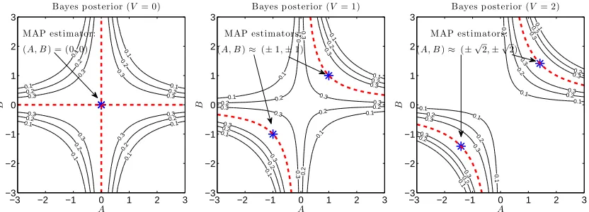
Figure 4: Bayes posteriors with ca=cb=100 (i.e., almost flat priors). The asterisks are the MAP solutions, and the dashed lines indicate the ML solutions (the modes of the contour when

ca=cb=c→∞).

0.1 0.1 0.1 0.1 0.1 0.1 0.1 0.1 0.2 0.2 0.2 0.2 0.2 0.2 0.2 0.3 0.3 0.3 0.3 A B

Bayes p osterior (V = 0)

−3 −2 −1 0 1 2 3

−3 −2 −1 0 1 2 3 0.1 0.1 0.1 0.1 0.1 0.1 0.1 0.1 0.2 0.2 0.2 0.2 0.2 0.2 0.2 0.3 0.3 A B

Bayes p osterior (V= 1)

−3 −2 −1 0 1 2 3

−3 −2 −1 0 1 2 3 0.1 0.1 0.1 0.1 0.1 0.1 0.1 0.1 0.1 0.1 0.2 0.2 0.2 0.2 A B

Bayes p osterior (V = 2)

−3 −2 −1 0 1 2 3

−3 −2 −1 0 1 2 3

Figure 5: Bayes posteriors with ca=cb=2. The dashed lines indicating the ML solutions are

identical to those in Figure 4.

4.1 MAPMF

First, we illustrate the behavior of the MAP estimator.

When L=M=H=1, Equation (17) yields that the Bayes posterior p(A,B_|V)is given as

p(A,B_|V)∝exp

−_2σ12(V−BA) 2 − A 2 2c2 a− B2

2c2_b

. (53)

Figure 4 shows the contour of the above Bayes posterior when V =0,1,2 are observed, where the

noise variance isσ2=1 and the hyperparameters are ca=cb=100 (i.e., almost flat priors). When

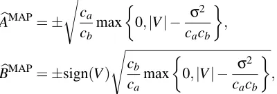
For finite caand cb, Theorem 1 and Equation (66) (in Appendix B) imply that the MAP solution can be expressed as

b

AMAP=_±

s ca

cb max

0,_|V_{| −} σ

2

cacb

,

b

BMAP=_±sign(V)

s cb

ca max

0,_|V| − σ2

cacb

,

where sign(_·)denotes the sign of a scalar. In Figure 4, the asterisks indicate the MAP estimators, and the dashed lines indicate the ML estimators (the modes of the contour of Equation (53) when

ca=cb=c→∞). When V=0, the Bayes posterior takes the maximum value on the A- and B-axes,

which results inUbMAP=0. When V =1, the profile of the Bayes posterior is hyperbolic and the

maximum value is achieved on the hyperbolic curves in the positive orthant (i.e., A,B>0) and the negative orthant (i.e., A,B<0); in either case,UbMAP_≈1 (andUbMAP_→1 as ca,cb→∞). When

V =2, a similar multimodal structure is observed and the solution isUbMAP_≈2 (andUbMAP_→2 as

ca,cb→∞). From these plots, we can visually confirm that the MAP solution with almost flat priors (ca=cb=100) approximately agrees with the ML solution:UbMAP≈UbML=V (andUbMAP→UbML as ca,cb→∞).

Furthermore, these graphs illustrate the reason why the product cacb→∞is sufficient for MAP to agree with ML in the MF setup (see Section 3.1). Suppose cais kept small, say ca=1, in Figure 4. Then the Gaussian ‘decay’ remains along the horizontal axis in the profile of the Bayes posterior.

However, the MAP solutionUbMAP does not change since the mode of the Bayes posterior is kept

lying on the dashed line (equivalence class). Thus, MAP agrees with ML if either caor cbtends to infinity.

Figure 5 shows the contour of the Bayes posterior when ca=cb=2. The MAP estimators are

shifted from the ML estimators (dashed lines) toward the origin, and they are more clearly contoured as peaks.

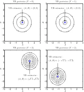
4.2 VBMF

Here, we illustrate the behavior of the VB estimator, where the Bayes posterior is approximated by a spherical Gaussian.

In the current one-dimensional setup, Corollary 1 implies that the VB posteriors rA(A_|V)and

rB(B|V)can be expressed as

rA(A|V) =

N

q bγVB_c

a/cb,ζca/cb),

rB(B|V) =

N

q bγVB_c

b/ca,ζcb/ca),

where

N

s bγVB

2 +

σ2 2cacb

2 +σ2₋

bγVB

2 +

σ2 2cacb

,

bγVB₌

  

max

0,

1₋σ

2

V2

|V_{| −} σ

2

cacb

if V ₆=0,

0.05

0.05

0.05

0.05

0.05

0.05

0.05

0.1

0.1

0.1

0.1 0.15 0.15

A

B

VB p osterior (V= 0)

−3 −2 −1 0 1 2 3

−3 −2 −1 0 1 2 3

VB estimator : (A, B) = (0,0)

0.05

0.05

0.05

0.05

0.05

0.05

0.05

0.1

0.1

0.1

0.1 0.15 0.15

A

B

VB p osterior (V = 1)

−3 −2 −1 0 1 2 3

−3 −2 −1 0 1 2 3

VB estimator : (A, B) = (0,0)

0.05

0.05

0.05 0.05

0.05

0.05

0.1 0.1

0.1 0.1

0.1

0.15 0.15 0.15

0.15

0.2

0.2 0.2

0.25

0.25

0.3

A

B

VB p osterior (V= 2)

−3 −2 −1 0 1 2 3

−3 −2 −1 0 1 2 3

VB estimator :

(A, B)≈(√1.5,√1.5)

0.05

0.05

0.05

0.05

0.05

0.05

0.1 0.1

0.1

0.1 0.1

0.15

0.15

0.15

0.15

0.2

0.2 0.2

0.25

0.25 0.3

A

B

VB p osterior (V = 2)

−3 −2 −1 0 1 2 3

−3 −2 −1 0 1 2 3

VB estimator :

(A, B)≈(−√1.5,−√1.5)

Figure 6: VB posteriors and VB solutions when L=M=1 (i.e., the matrices V , U , A, and B are

scalars). When V =2, VB gives either one of the two solutions shown in the bottom row.

Figure 6 shows the contour of the VB posterior r(A,B_|V) =rA(A|V)rB(B|V)when V =0,1,2 are observed, where the noise variance isσ2=1 and the hyperparameters are ca=cb=100 (i.e.,

almost flat priors). When V =0, the cross-shaped contour of the Bayes posterior (see Figure 4)

is approximated by a spherical Gaussian function located at the origin. Thus, the VB estimator is

b

UVB=0, which is equivalent to the MAP solution. When V =1, two hyperbolic ‘modes’ of the

Bayes posterior are approximated again by a spherical Gaussian function located at the origin. Thus, the VB estimator is stillUbVB=0, which is different from the MAP solution.

V=eγVB

h ≈

√

Mσ2_{=1 (e}γVB

h →

√

Mσ2_{as c}

a,cb→∞) is actually a transition point of the behavior

of the VB estimator. When V is not larger than the threshold √Mσ2_{, the VB method tries to}

approximate the two ‘modes’ of the Bayes posterior by the origin-centered Gaussian function. When

V goes beyond the threshold√Mσ2_{, the ‘distance’ between two hyperbolic modes of the Bayes}

posterior becomes so large that the VB method chooses to approximate one of the two modes in the positive and negative orthants. As such, the symmetry is broken spontaneously and the VB solution

is detached from the origin. Note that, as discussed in Section 3, Mσ2 _{amounts to the expected}

contribution of noise

E

The bottom row of Figure 6 shows the contour of two possible VB posteriors when V =2. Note

than the MAP solutionUbMAP=2, and the difference between the VB and MAP solutions tends to shrink as V increases.

4.3 EVBMF

Next, we illustrate the behavior of the EVB estimator.

In the current one-dimensional setup, the free energy (39) is expressed as

FVB(r|V,c2a,c2b) =log

c2_ac2_b

ΣaΣb

+µ 2 a+Σa

2c2 a

+µ 2 b+Σb

2c2_b

−_σ12V µaµb+ 1

2σ2 µ

2

a+Σa µ2b+Σb+Const.

According to Corollary 2, if_|V_{| ≥}2σandϕ(_|V_|)_≤0, the EVB estimator of the hyperparameters is given by

(_bcEVB_a )2= (c_bbEVB)2=_|V_|ρ+, (54)

where

ϕ(_|V|) =log

|V_|2

σ2 (1−ρ−)

−|V|

2

σ2 (1−ρ−) +

1+|V| 2 2σ2ρ

2

+

,

ρ_±=

v u u

t1

2 1−

σ2

|V_|2±

s

1₋4σ

2

|V_|2

!

.

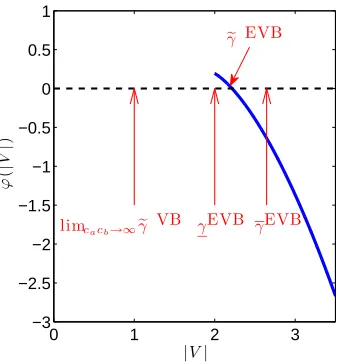
Based on a simple numerical evaluation (Figure 7) ofϕ(_|V|), we can confirm that Equation (54) holds if_|V_{| ≥}eγEVB_{, where}

eγEVB

≈2.22.

Otherwisec_bEVB_ah ,_bcEVB_b

h →0. Note thateγ

EVB_{is theoretically bounded as}

2=2σ2=γEVB_≤eγEVB

≤γEVB=√7σ2_≈2.64

,

as shown in Equation (52).

Using Corollary 1 with Equation (54), we can plot the EVB posterior. When

|V_|<eγEVB

≈2.22,

the infimum of the free energy with respect to (µa,µb,Σa,Σb,c2a,c2b) is attained by c2a =c2b =ε,

µa=µb=0, and

Σa=Σb= σ2 2ε

r

1+4nε2 σ2 −1

!

,

whereε_→0 (i.e., c2

0 1 2 3 −3

−2.5 −2 −1.5 −1 −0.5 0 0.5 1

|V|

ϕ

(

|

V

|

)

limcacb→∞eγ VB γEVB γEVB

e

γ EVB

Figure 7: Numerical evaluation ofϕ(_|V_|)when L=M=1 andσ2=1 (the blue solid curve). The blue solid curve crosses the black dashed line (ϕ(_|V_|) =0) at_|V_|=eγEVB_≈2.22.

is observed, where the noise variance isσ2=1. SinceUbMAP_≈2 andUbVB_≈1.5 under almost flat

priors (see Figure 4 and Figure 6),UbEVB_{=0 is more strongly regularized than VB and MAP.}

On the other hand, when

|V_{| ≥}eγEVB

≈2.22,

the EVB posteriors rA(A|V)and rB(B|V)can be expressed as

rA(A|V) =

N

q

bγEVB_,ζ_),

rB(B|V) =

N

q

bγEVB_,ζ_), where

ζ=

s bγEVB

2 +

|V_|ρ₋

2

2 +σ2₋

bγEVB

2 +

|V_|ρ₋

2

,

ρ₋=

v u u

t1

2 1−

2σ2 γ2

h

−

s

1₋4σ

2 γ2

h

!

,

bγEVB₌

1−σ

2

V2−ρ−

|V|.

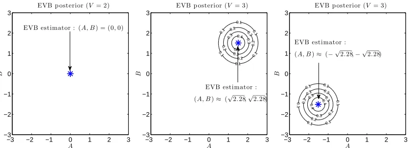
When V=3 is observed, we haveUbEVB_≈2.28 (c2_a=c2_b≈2.62, µa=µb≈

√

2.28, andΣa=Σb≈

0.33). The possible posteriors are plotted in the middle and the right graphs of Figure 8. Since

b

−3 −2 −1 0 1 2 3 −3

−2 −1 0 1 2 3

A

B

EVB p osterior (V = 2)

EVB estimator : (A, B) = (0,0)

0.1 0.1

0.1

0.1 0.1

0.1

0.2

0.2 0.2

0.2 0.2

0.3

0.3

0.3

0.4 0.4

A

B

EVB p osterior (V= 3)

−3 −2 −1 0 1 2 3

−3 −2 −1 0 1 2 3

EVB estimator :

(A, B)≈(√2.28,√2.28)

0.1 0.1

0.1

0.1

0.1

0.1

0.2 0.2

0.2 0.2

0.2

0.3 0.3

0.3 0.4 0.4

A

B

EVB p osterior (V = 3)

−3 −2 −1 0 1 2 3

−3 −2 −1 0 1 2 3

EVB estimator :

(A, B)≈(−√2.28,−√2.28)

Figure 8: EVB posteriors and EVB solutions when L=M=1. Left: When V =2, the EVB

posterior is reduced to Dirac’s delta function located at the origin. Right: When V =3,

the solution is detached from the origin and given by(A,B)_≈(√2.28,√2.28)or(A,B)_≈ (₋√2.28,₋√2.28), which both yields the same solutionUbEVB_≈2.28.

4.4 FBMF

Here, we illustrate the behavior of the FB estimator.

When L=M=H=1, the FB solution (5) is expressed as

b

UFB=_hAB_ip(V|A,B)φA(A)φB(B). (55)

If V =0,1,2,3 are observed, the FB solutions with almost flat priors are 0,0.92,1.93,2.95,

re-spectively, which were numerically computed.2 Since the corresponding MAP solutions (with the

almost flat priors) are 0,1,2,3, FB and MAP were shown to produce different solutions.

The theory by Jeffreys (1946) explains the origin of model-induced regularization in FB. Let us consider the non-factorizing model

p(V_|A,B)∝exp

−_2σ1₂kV₋U_k2_Fro

, (56)

where U itself is the parameter to be estimated. The Jeffreys (non-informative) prior for this model is uniform

φJef

U (U)∝1. (57)

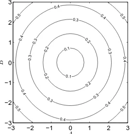
On the other hand, the Jeffreys prior for the MF model (1) is given by

φJef

A,B(A,B)∝

p

A2_+B2_{, (58)}

which is illustrated in Figure 9 (see Appendix I for the derivation of Equations (57) and (58)). Note thatφJef_U (U)andφJef_A,B(A,B)are both improper.

0.1

0.1

0.2

0.2 0.2

0.2

0.3

0.3 0.3 0.3 0.3

0.3

0.4

0.4

0.4

0.4

0.4 0.4

0.4 0.5

0.5

0.5

0.5

A

B

−3 −2 −1 0 1 2 3

−3 −2 −1 0 1 2 3

Figure 9: The Jeffreys non-informative prior of the MF model in the joint space of A and B: φJef(A,B)∝√A2_+B2_{. The scaling of the density value in the graph is arbitrary due} to impropriety.

Jeffreys (1946) states that the both combinations, the non-factorizing model (56) with its Jeffreys prior (57) and the MF model (1) with its Jeffreys prior (58), give the equivalent FB solution. We can easily show that the former combination, Equations (56) and (57), gives an unregularized solution. Thus, the FB solution in the MF model (1) with its Jeffreys prior (58) is also unregularized. Since the flat prior on(A,B)has more probability mass around the origin than the Jeffreys prior (58) (see Figure 9), it favors smaller_|U_|and regularizes the FB solution.

4.5 EMAPMF

As explained in Section 3.3, EMAPMF always results in the trivial solution, A,B=0 and cah,cbh →

0.

4.6 EFBMF

The EFBMF solution is written as follows:

b

UEFB=_hAB_ip(V|A,B)φA(A;bca)φB(B;bcb),

where

(_bca,bcb) =argmin

(ca,cb)

F(V ; ca,cb).

Here F(V ; ca,cb)is the Bayes free energy (6).

When V =0,1,2,3 are observed, the EFB solutions are 0,0.00,1.25,2.58 (_bca=cbb≈0,0.0,1.4, 2.1), respectively, which were numerically computed.3 Since F(V ; ca,cb)→∞when cacb→∞, the

3. The model (1) and the priors (2) and (3) are invariant under the following parameter transformation

(a_h,b_h,ca

h,cbh)→(s 1/2

h ah,s−

1/2

h bh,s

1/2

h cah,s

−1/2

h cbh)

for any{sh∈R_{; sh>0,h=1, . . . ,H}. Here, we fixed the ratio to ca/cb=1. For cacb=10}−2.00_,10−1.99_{, . . . ,10}1.00_,

1 2 3 1

2 3

V

bU

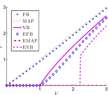
FB MAP VB EFB EMAP EVB

Figure 10: Numerical results of the FBMF solutionUbFB, the MAPMF solutionUbMAP, the VBMF

solution UbVB, the EFBMF solution UbEFB, the EMAPMF solution UbEMAP, and the

EVBMF solutionUbEVBwhen the noise variance isσ2=1. For MAPMF, VBMF, and

FBMF, the hyperparameters are set to ca=cb=100 (i.e., almost flat priors).

minimizer of F(V ; ca,cb)with respect tobca andcbbare always finite. This implies that EFBMF is more strongly regularized than FBMF with almost flat priors (cacb→∞).

4.7 Summary

Finally, we summarize the numerical results of all Bayes estimators in Figure 10, including the

FBMF solutionUbFB, the MAPMF solutionUbMAP, the VBMF solutionUbVB, the EFBMF solution

b

UEFB, the EMAPMF solutionUbEMAP, and the EVBMF solutionUbEVB when the noise variance is

σ2_{=1. For MAPMF, VBMF, and FBMF, the hyperparameters are set to c}

a=cb=100 (i.e., almost flat priors). Overall, the solutions satisfy

b

UEMAP_≤UbEVB_≤UbEFB_≤UbVB_≤UbFB_≤UbMAP,

which shows the strength of regularization effect of each method.

5. Conclusion

In this paper, we theoretically analyzed the behavior of Bayesian matrix factorization methods. More specifically, in Section 3, we derived non-asymptotic bounds of the maximum a posteriori

ma-trix factorization (MAPMF) estimator and the variational Bayesian mama-trix factorization (VBMF)

estimator. Then we showed that MAPMF consists of the trace-norm shrinkage alone, while VBMF consists of the positive-part James-Stein (PJS) shrinkage and the trace-norm shrinkage.

as the Gaussian distribution in the space of the target matrix produce highly complicated multimodal distributions in the space of factorized matrices.

We further extended the above analysis to empirical VBMF scenarios where hyperparameters included in priors are optimized based on the VB free energy. We showed that the ‘strength’ of the PJS shrinkage is more than doubled compared with the flat prior cases. We also illustrated the behavior of Bayesian matrix factorization methods using one-dimensional examples in Section 4.

Our theoretical analysis relies on the assumption that a fully observed matrix is provided as a training sample. Thus, our results are not directly applicable to the collaborative filtering scenarios where an observed matrix with missing entries is given. Our important future work is to extend the current analysis so that the behavior of the collaborative filtering algorithms can also be explained. The correspondence between MAPMF and the trace-norm regularization still holds even if missing entries exist. Likewise, we hope to find a relation between VBMF and a regularization term acting on a matrix, which results in the PJS shrinkage if a fully observed matrix is given.

Our analysis also relies on the column-wise independence constraint (14), which was also used in Raiko et al. (2007), on the VB posterior. In principle, the weaker matrix-wise constraint (9) which was used in Lim and Teh (2007) allows non-zero covariances between column vectors, and can achieve a better approximation to the true Bayes posterior. How this affects the performance and when the difference is substantial are to be investigated.

As explained in Appendix A, the PJS estimator dominates (i.e., uniformly better than) the

max-imum likelihood (ML) estimator in vector estimation. This means that, when L=1, VBMF with

(almost) flat priors dominates MLMF. Another interesting future direction is to investigate whether this nice property is inherited to matrix estimation. For matrix estimation (L>1), a variety of estimators which shrink singular values have been proposed (Stein, 1975; Ledoit and Wolf, 2004; Daniels and Kass, 2001), and were shown to possess nice properties under different criteria. Dis-cussing the superiority of such shrinkage estimators including VBMF is interesting future work.

Our investigation revealed a gap between the fully-Bayesian (FB) estimator and the VB estima-tor (see Section 4.7). Figure 10 showed that the VB estimaestima-tor tends to be strongly regularized. This could cause underfitting and degrade the performance. On the other hand, it is also possible that, in some cases, this stronger regularization could work favorably to suppress overfitting, if we take into account the fact that practitioners do not always choose their prior distributions based on explicit prior information (it is often the case that conjugate priors are chosen only for computational con-venience). Further theoretical analysis and empirical investigation are needed to clarify when the stronger regularization of the VB estimator is harmful or helpful.

Tensor factorization is a high-dimensional extension of matrix factorization, which gathers

con-siderable attention recently as a novel data analysis tool (Cichocki et al., 2009). Among various methods, Bayesian methods of tensor factorization have been shown to be promising (Tao et al., 2008; Yu et al., 2008; Hayashi et al., 2009; Chu and Ghahramani, 2009). In our future work, we will elucidate the behavior of tensor factorization methods based on a similar line of discussion to the current work.

Acknowledgments

Appendix A. James-Stein Shrinkage Estimator

Here, we briefly introduce the James-Stein (JS) shrinkage estimator and its variants (James and Stein, 1961; Efron and Morris, 1973).

Let us consider the problem of estimating the meanµ(_∈Rd_{)of the d-dimensional Gaussian}

distribution

N

d)from its independent and identically distributed samples

X

{xi∈Rd|i=1, . . . ,n}.

We measure the generalization error (or the risk) of an estimatorµbby the expected squared error:

E_kµb−µk2_,

whereE_{denotes the expectation over the samples}

X

An estimatorµ_bis said to dominate another estimatorµ_b′if

E_kµb−µk2_≤E_kµb′_−µk2_{for allµ,}

and

E_kµb−µk2_<E_kµb′_−µk2_{for someµ.}

An estimator is said to be admissible if no estimator dominates it.

Stein (1956) proved the inadmissibility of the maximum likelihood (ML) estimator (or equiva-lently the least-squares estimator),

b

µML=1

n

n

∑

i=1

xi,

when d≥3. This discovery was surprising because the ML estimator had been believed to be a

good estimator. James and Stein (1961) subsequently proposed the JS shrinkage estimator µ_bJS,

which was proved to dominate the ML estimator:

b

µJS=

1₋ χσ

2

n_kµ_bML_k2

b

µML, (59)

whereχ=d₋2. Efron and Morris (1973) showed that the JS shrinkage estimator can be derived as

an empirical Bayes estimator. In the current paper, we refer to all estimators of the form (59) with arbitraryχ>0 as the JS shrinkage estimators.

The positive-part James-Stein (PJS) shrinkage estimator, which was shown to dominate the JS estimator, is given as follows (Baranchik, 1964):

b

µPJS=max

0,

1₋ χσ

2

n_kµ_bML_k2

b

µML

.