Application of Binary Logistic Regression Model to Assess the Likelihood of Overweight

http://www.sciencepublishinggroup.com/j/ajtas doi: 10.11648/j.ajtas.20190801.13

ISSN: 2326-8999 (Print); ISSN: 2326-9006 (Online)

Application of Binary Logistic Regression Model to Assess

the Likelihood of Overweight

Noora Shrestha

Department of Mathematics and Statistics, P. K. Multiple Campus, Tribhuvan University, Kathmandu, Nepal

Email address:

To cite this article:

Noora Shrestha. Application of Binary Logistic Regression Model to Assess the Likelihood of Overweight. American Journal of Theoretical and Applied Statistics. Vol. 8, No. 1, 2019, pp. 18-25. doi: 10.11648/j.ajtas.20190801.13

Received: January 19, 2019; Accepted: February 20, 2019; Published: March 6, 2019

Abstract:

This study attempts to assess the likelihood of overweight and associated factors among the young students by analyzing their physical measurements and physical activity index. This paper has classified four hundred and fifteen subjects and precisely estimated the likelihood of outcome overweight by combining body mass index and CUN-BAE calculated. Multicollinearity is tested with multiple regression analysis. Box-Tidwell Test is used to check the linearity of the continuous independent variables and their logit (log odds). The binary regression analysis was executed to determine the influences of gender, physical activity index, and physical measurements on the likelihood that the subjects fall in overweight category. The sensitivity and specificity described by the model are 55.9% and 96.9% respectively. The increase in the value of waist to height ratio and neck circumference and drop in physical activity index are associated with the increased likelihood of subjects falling to overweight group. The prevalence of overweight is higher (27.8%) in female than in male (14.7%) subjects. The odds ratio for gender reveals that the likelihood of subjects falling to overweight category is 2.6 times higher in female compared to male subjects.

Keywords:

Overweight, Waist to Height Ratio, Neck Circumference, Binary Logistic Model, Odds Ratio

1. Introduction

Overweight and obesity has become a major public health problem from the last two decades in the world. The worldwide problem of overweight and obesity has affected the individual, family, society, and the nation. The prevalence of overweight people in 1990 was 8.1% men and 9.4% women [1]. The prevalence of overweight and obesity in Nepal has been mounting significantly for the past 26 years. The proportion of overweight and obesity were 12% and 1.7% respectively in the age group 15 to 29 years for both genders. The percentage of overweight and obesity in female (12.3% & 2%) was higher than in male (11.8% &1.5%) on the basis of Body Mass Index (BMI) [2]. Similar results of overweight continued in Nepal demographic and health survey, 2016. This survey observed 22% of female and 17% of male were overweight (BMI ≥ 25 kg/m2), at the age group 15-49 years [3].

The prevalence of overweight is different on the basis of age, sex, and location division of the samples [4]. The uppermost percentage is observed among women from the

richest families (45%) and from the Province 3, 35% of them were reported to be overweight or obese. Among men, 28% at age 30-39 years and 32% from wealthiest families are more prone to be overweight or obese [5]. The prevalence of overweight or obesity is also expected to differ by its method of estimation. There are various ways to measure overweight or obesity. The field methods are waist circumference, waist to hip ratio, skinfold thickness, bioelectrical impedance, and densitometry [6].

scan, and dual energy x-ray absorptiometry [8]. The previous studies show that there is no specific cutoff point of obesity or overweight for Asian young adult group as it differs with various factors and this group has lower BMI but higher body fat percentage [9].

To succeed in dealing with limitation of BMI for categorization, this paper has combined the value of BMI and body fat percentage to classify the subject in overweight or no overweight group and further precisely estimate the likelihood of overweight [10].

The several research studies have mentioned that overweight and obesity are major reasons of co-morbidities, diabetes, heart disease, cancer, and other health problems. The related health care cost is also a significant factor. The urban lifestyle, overreliance on technology, and less focus on physical activities bring health related problems such as overweight or obesity among the young students [10-11]. This raises the question about prevalence and contributing factors about overweight using simple and cost effective screening method in young students.

With the consideration of this fact, the present paper attempts to assess the likelihood of overweight and its associated factors among the young students by applying binary logistic regression model.

2. Materials and Methods

The analysis and discussion of this paper were based on the output of statistical analysis performed by using IBM SPSS 23 for Windows. The study protocol was approved by the ethical and research committee of the Dayananda Anglo Vedic College, Bhanimandal, Nepal. This is a cross sectional study conducted over a period of three months (June to August) in 2018. The sample consisted of four hundred and fifteen subjects (170 Male and 245 Female) that had been obtained using convenience sampling method. The subjects with the written consent, residing in the same urban area, not having serious health issues, studying in bachelor’s level, and an age from eighteen to twenty three years were inclusionary criteria.

2.1. Measurements and Variables

For all the subjects, the physical measurements were recorded by the researcher to negate any inter observer variability. The explanatory variables height, weight, neck circumference, waist circumference and hip circumference were measured by the researcher on the basis of the report of WHO expert consultation [8]. Body Mass Index (BMI) was calculated dividing weight in kg by height in m2. The subjects were asked to fill a form that includes the activities for intensity, duration, and frequency of physical activity. The physical activity score was calculated by finding the product of intensity, duration and frequency of activity. The physical activity index (PAI) was categorized into high, very good, fair and poor [8, 12].

The measurement of body fat percentage (BF%) using sophisticated equipment was restricted for the subjects under

study. Thus, this study had calculated BF% using equation of Clinica Universidad de Navarra- Body Adiposity Estimator (CUN-BAE). The researchers claimed that CUN-BAE has validated an easy to apply projecting equation, which may be applied as a primary screening tool in clinical practice.

Body Fat % = − 44.988 + (0.503 × age) + (10.689 × sex) + (3.172 × BMI) - (0.026 × BMI2) + (0.181 × BMI × sex) - (0.02 × BMI × age) - (0.005 × BMI2 × sex) + (0.00021 × BMI2 × age), where, BMI = body mass index, male = 0 and female = 1 for sex and age in years [13-14].

This study considered a dichotomous outcome variable overweight or no overweight. To improve the classification of subjects and more specifically estimate the likelihood of overweight, BMI, and BF% were combined. The female subjects whose BMI ≥ 25 kg/m2 correspond to body fat > 32% were classified into overweight group and BMI < 25 kg/m2 correspond to body fat ≤ 32% were classified into no overweight group. Considering BMI ≥ 25 kg/m2 correspond to body fat > 23%, the male subjects were classified into overweight group and BMI < 25 kg/m2 correspond to body fat ≤ 23% were classified into no overweight group [10, 15, 16].

2.2. Statistical Analysis

Pearson's correlation coefficient was used to determine the relationship between BMI and BF% with the continuous explanatory variables. The association between the outcome variable overweight/ no overweight and categorical independent variables was examined using Pearson Chi Square test. Phi and Cramer’s V tests were used to test the strength of association between the variables. The prevalence of overweight was calculated as dividing the number of subjects who was classified in overweight (or no overweight) by the number of subjects in whom it was measured, and expressed as a percentage. To check the linearity of the continuous independent variables and the logit (log odds) transformation, Box- Tidwell Test was used. Multiple regression model was applied to test the multicollinearity of the variables [17-18].

A binary logistic regression analysis has been applied to predict the likelihood that a subject falls into any one of the two groups of a dichotomous dependent variable (overweight or no overweight) based on the independent variables that were continuous, and categorical. The reasons for selecting this model were i) it is particularly flexible and ii) gives momentous interpretation in health studies [19-20].

Let us assume that a sample of n independent observations of the pair (xi, yi), i = 1,2,….n. The probability distribution of

the outcome variable is Binomial i.e. yi ~ Bin (ni, π(xi))

where, yi denote the value of a dichotomous response

variable, and xi denotes the value of the independent variable

for the ith subject. Now,

Let us consider the conditional mean, as π(x), the expected value of y given the value of x in logistic regression:

π x =_#$ !" _!" (1)

To fit the logistic regression model in equation (1) to a set of data, the unknown parameters β0 and β1 have to be

estimated and for dichotomous data, 0 ≤ π(x) ≤1. The binary regression model intends to predict the logit, which is the natural log of the odds of subjects to be overweight or no overweight with predictors such as gender, physical measurement, and physical activity index. The term logit transformation in this model is the transformation of π(x) which is defined as:

logit π x = ln '_{#*( )}( ) + = β-+ β#x (2)

Here, π(x) is the predicted probability of the event which is coded with “1” overweight rather than “0” no overweight. 1- π(x) is the predicted probability of the other decision and x is the independent variable. The logit value may be continuous and range from -∞ to +∞. The expression for π(x) in equation (1) provides the conditional probability P (Y=1|x) and the term 1- π(x) gives the conditional probability P(Y= 0|x) for an arbitrary parameter β = β0 and β1, the vector

parameters. For those pairs (xi, yi), if yi = 1, the contribution

to the likelihood function is π(xi), and if yi = 0, it is 1- π(xi);

where π(xi) is the value of π(x) computed at xi [21]. It can be

expressed as:

/ 01 2341 − / 01 6#*23 ₍₃₎

For logistic regression, the observations are assumed to be independent, so the likelihood function is obtained as follows:

l β = ∏ π x:_;# 8941 − π x 6#*89 ₍₄₎

For ease of mathematical calculations, log of equation (4), log likelihood, can be written as:

L β = ln4l β 6 = ∑ {y ln4π x 6 +:

;# 1 − y ln 41 −

π x 6} (5) Differentiating equation (5) with respect to β0 and β1 for

maximizing likelihood function, L (β) and solving for βwe get the two likelihood equations as:

∑4y − π x 6 = 0 (6)

∑ x 4y − π x 6 = 0 (7) For binary logistic regression the terms in equations (6) and (7) are non linear in β0 and β1, and hence require iterative

methods for solution which is obtained by using an iterative weighted least square technique. Then, the value of maximum likelihood estimate @A will be obtained [22]. In the

present study, there is few major independent variables such as gender, physical measurement, physical activity index for which the expression of binary logistics regression model (i= 1,2,…, n subjects) is given by

ln ' ( )9

#*( )₉+ = β-+ β#x#+ βBxB+ ⋯ β:x: (8)

Here, xi1, xi2. ….xin are categorical or continuous

independent variables [23]. From equation (8), the equation for the prediction of the probability can be derived and solved the logit equation for π(xi) to obtain

π x =_{1 + e}eD $D_{D $D}!)9!_!)$D_9!$DE)9E_E)$⋯D_9E$⋯DF)9F_F)9F

3. Results and Discussions

For the exposure of multicollinearity, the Pearson’s correlation coefficients (r) between each pair of continuous independent variables are observed in Table 1. It is assumed that there is no multicollinearity because there is no high degree of correlation among the independent variables. Nevertheless, the correlation coefficient value between the independent variables may be deliberated as the sufficient, but not the necessary condition for the multicollinearity [24].

Table 1 shows the coefficient of determination (R2) value calculated for the pairwise independent variables waist to hip ratio (whr), neck circumference (nc), physical activity index (PAI), and waist to height ratio (whtr). The R2 values of each combination of independent variables may deliver the noticeable indication for the presence of multicollinearity. The value of R2 is low for the pairs that show there is less chance of presence of multicollinearity but this cannot be pondered as the best test for perceiving multicollinerity.

In case of female subjects, it has been observed that there is positive and significant relationship between BMI and independent variables namely neck circumference, waist to hip ratio, waist to height ratio with p < 0.01. There is significant negative correlation between BMI and physical activity index. Similarly, BF% is significantly and positively correlated with all these independent variables and negatively correlated with physical activity index at the p < 0.01 level.

Table 1. Result of Pearson’s Correlation.

Variables

BMI BF%

Female Male Female Male

r R2 _{r R}2 _{r R}2 _{r R}2

whr 0.324 0.105 0.026+ _{0.00067 0.338 0.114 0.018}+ _0.00033

nc 0.457 0.209 0.168 0.028 0.375 0.141 0.166 0.028

whtr 0.658 0.433 0.488 0.238 0.641 0.411 0.483 0.233

PAI -0.32 0.106 -0.31 0.101 -0.28 0.079 -0.309 0.095

BMI 1 1 1 1 0.911 0.83 0.998 0.996

BF% 0.911 0.83 0.998 0.996 1 1 1 1

Correlation is significant at the 0.01 level (2-tailed)

whr- waist to hip ratio, nc- Neck Circumference, whtr- waist to height ratio, PAI- Physical activity index, BMI- Body mass index, BF%- Body fat percentage, + Correlation is not significant

Table 2 presents the dichotomous categorical variables that are obtained by classification of subjects on the basis of the measurements [8]. The Chi Square test in table 2 demonstrates that there is statistically significant association between weight status category of female and the categorical variables whr_cat, nc_cat, and whtr_cat with p = 0.0001. Phi and Cramer’s V tests depict that the strength of association between the variables is very strong in female subjects (p = 0.0001).

Table 2. Result of Chi Square Test.

Categorical

Variables Gender Category

Weight Status Category

Pearson Chi- Square (p value)

Phi and Cramer’s V(p value)

No Overweight Overweight

n, % n, %

Waist to hip ratio (whr_cat)

Female No Risk 168, 80.4% 41, 19.6% 0.000

Risk (≥ 0.85) 9, 25% 27, 75% 0.000

Male No Risk 122, 88.4% 16, 11.6% 0.026 0.017

Risk (≥ 0.90) 23, 71.9% 9, 28.1%

Neck Circumference (nc_cat)

Female No Overweight 161, 85.6% 27, 14.4% 0.000

Overweight (≥ 34 cm) 16, 28.1% 41, 71.9% 0.000

Male No Overweight 113, 86.3% 18, 13.7% 0.606

Overweight (≥ 37 cm) 32, 82.1% 7, 17.9% 0.515

Waist to height ratio (whtr_cat)

Female No Overweight 155, 88.1% 21, 11.9% 0.000

Overweight (≥ 0.49) 22, 31.9% 47, 68.1% 0.000

Male No Overweight 136, 89.5% 16, 10.5% 0.000 0.000

Overweight (≥ 0.53) 9, 50% 9, 50%

Gender Female 177, 72.2% 68, 27.8% 0.002 0.002

Male 145, 85.3% 25, 14.7%

In case of male subjects, Chi Square test and Phi & Cramer’s V tests reveal that there is statistically significant and very strong association between weight status category and the categorical variables based on waist to hip ratio and waist to height ratio with p = 0.0001. The strength of association is very weak between weight status category and neck circumference category in male subjects with p > 0.05. The strength of association between weight status category and gender is statistically significant and very strong with p = 0.002.

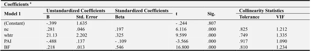
Table 3 illustrates the output of multiple regression model,

which has been used to further test the multicollinearity among the independent variables. In multiple regression, multicollinearity can be identified by two collinearity diagnostic factors; tolerance and variance inflation factor (VIF). Regarding tolerance, all the independent variables have more than 0.1 tolerance value in the output of coefficients. The VIF values are also less than 10, which indicate that there is no presence of multicollinearity in the model. Similar results obtained when outcome variable is changed in multiple regression model such as BF%.

Table 3. Result of Multiple Regression Analysis.

Coefficients a

Model 1 Unstandardized Coefficients Standardized Coefficients t Sig. Collinearity Statistics

B Std. Error Beta Tolerance VIF

(Constant) -.399 1.635 - .244 .807

nc .281 .046 .197 6.116 .000 .825 1.212

whtr 21.13 2.202 .325 9.599 .000 .749 1.335

PAI -.488 .137 - .109 -3.566 .000 .917 1.090

BF .218 .013 .546 16.800 .000 .810 1.234

a. Dependent Variable: BMI

result of the model.

(1)The categorical dependent variable has been measured on dichotomous scale using “0” for no overweight and “1” for overweight.

(2)The independent variables are continuous and categorical and not necessarily linearly related with dependent variable. This can be witnessed by multiple regression table 3.

(3)There is independence of observations. The independent variables are not highly correlated with each other. This can be observed by Pearson’s correlation in table 1.

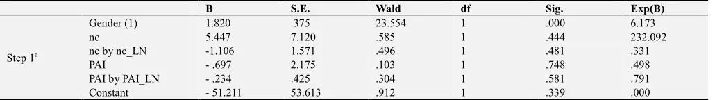
(4)There is a linear association between the continuous independent variables and their logit (log odds). This can be noticed by result of Box- Tidwell test in table 4. Table 4 demonstrates the output of Box–Tidwell Test, which has been used to test the assumption of linearity of the

continuous variables. Before using binary logistic regression model, it is assumed that the relationship between the continuous independent variables and the logit (log odds) is linear. This assumption is tested, by entering interactions between the continuous independent variables and their logs in the model. The interaction terms nc by nc_LN and PAI by PAI_LN are not significant (p = 0.481 and p = 0.581). It means there is linear association between the continuous independent variables neck circumference and physical activity index and the logit (log odds) with the outcome variable weight status category. Finally, waist to height ratio, neck circumference, physical activity index, and gender are selected as the suitable explanatory variables with outcome variable weight status category for the binary logistic regression model. Furthermore, the outputs of the binary logistic regression model are discussed.

Table 4. Result of Box – Tidwell Test.

B S.E. Wald df Sig. Exp(B)

Step 1a

Gender (1) 1.820 .375 23.554 1 .000 6.173

nc 5.447 7.120 .585 1 .444 232.092

nc by nc_LN -1.106 1.571 .496 1 .481 .331

PAI - .697 2.175 .103 1 .748 .498

PAI by PAI_LN - .234 .425 .304 1 .581 .791

Constant - 51.211 53.613 .912 1 .339 .000

a. Variables(s) entered on step 1: Gender, nc, nc *nc_LN, PAI, PAI*PAI_LN

Table 5 displays the output where 415 selected cases used in the analysis and no missing cases. There are two decision options, majority 322/415 = 77.6% subjects are in no overweight group, coded as “0” whereas, 93/415 = 22.4% cases are considered as overweight coded as “1”.

Table 5. Classification Tablea,b.

Observed

Predicted

Percentage Correct Weight Status Category

No Overweight Overweight

Step 0

Weight Status Category No Overweight 322 0 100.0

Overweight 93 0 .0

Overall Percentage 77.6

Constant is included in the model. The cut value is .500

Table 6 presents, Block 0: beginning block output variables in the equation, the intercept or constant only model which is ln(odds) = -1.242. By exponentiation on both sides of this expression, the predicted odds [Exp(B)] = Exp (-1.242) = 0.289. It means the predicted odds of overweight

subjects are 0.289. Since 93 subjects are overweight and 322 subjects are no overweight, the observed odds are 93/322 = 0.289. In this output, the other variables are not in the equation.

Table 6. Variables in the Equation.

B S.E. Wald Df Sig. Exp(B)

Step 0 Constant -1.242 0.118 111.3 1 .000 .289

Table 7 reports the result of an Omnibus test of model coefficients and demonstrates a Chi- square value of 188.863 on 4 degrees of freedom (df), significant at 0.0001. In Block 1: Method = enter output, the variables gender, neck circumference, waist to height ratio, and physical activity index are added as predictors. It shows a test of null hypothesis that adding the variables to the model has not significantly increased the ability to predict the weight status

of the study subjects.

Table 7. Omnibus Tests of Model Coefficients.

Chi-square df Sig.

Step 1

Step 188.863 4 .000

Block 188.863 4 .000

The output table 8 Model Summary presents the variation in the outcome variable weight status category explained by the independent variables with Cox and Snell R2 and Nagelkerke R2 (Pseudo R2) values. The Cox & Snell R2 = 0.366 shows 36.6% variation in outcome variable weight status category is explained by the predictors but the remaining 63.4% is unexplained. These R2 values demonstrate the explained variation in the outcome variable weight status category, by set of variables, ranges from 36.6% (Cox and Snell R2) to 55.8% (Nagelkerke R2). It also exhibits the -2 Log Likelihood statistic as 252.733. It measures how poorly the model predicts the decision; the smaller the statistic the better the model is. The block 0 model has the intercept 441.596. Adding variables to the model, the statistic -2 Log Likelihood is reduced by 441.596 – 252.733 = 188.863, which is Chi- square statistic.

Table 8. Model Summary.

Step -2 Log likelihood Cox & Snell R2 Nagelkerke R2

1 252.733a _{.366 .558}

a. Estimation terminated at iteration number 6 because parameter estimates changed by less than .001.

Table 9 presents the Hosmer-Lemeshow test, which tests the null hypothesis that the predictions made by the model fit absolutely with observed group memberships. A chi square statistic (8.389, d.f. = 8) was computed comparing the observed frequencies with those expected under the linear model. It shows the non-significant Chi Square value and indicates the model is good fit of data.

Table 9. Hosmer and Lemeshow Test.

Step Chi-square df Sig.

1 8.389 8 .396

Table 10 demonstrates the result of classification of subjects. Unlike multiple regression, binary regression model estimates the probability of a subject falling in an overweight or no overweight group. The cut value in the classification table is 0.5. The output classification table presents the grouping of the subject as overweight, if the projected probability of the event happening is ≥ 0.5. If the probability of the event of occurring is < 0.5, the subject is classified as no overweight. In the classification table, it can be observed that the overall success rate of the model has increased from 77.6% in block 0 to 87.7% in block 1.

Table 10. Classification Tablea_.

Observed

Predicted

Weight Status Category

Percentage Correct

No Overweight Overweight

Step 1 Weight Status Category

No Overweight 312 10 96.9

Overweight 41 52 55.9

Overall Percentage 87.7

a. The cut value is .500

The classification table 10 shows the percentage accuracy in classification is 87.7%. In addition, this value shows that 87.7% of cases are correctly classified as no overweight from the added independent variables.

The sensitivity = P (correct prediction| event did occur)= 52/93 = 55.9% or true positive value is the percentage of cases that had overweight and were acceptably anticipated by the model.

The specificity = P (correct prediction | event did not occur)= 312/322 = 96.9% or true negative value is the percentage of cases that did not have overweight and were appropriately projected as no overweight cases.

The false positive value = P (incorrect prediction| predicted occurrence) = 10/62 = 16.1% is the percentage of suitably

expected cases with the detected feature of no overweight compared to the total number of cases predicted as overweight.

The false negative value = P (incorrect prediction| predicted non-occurrence) = 41/353 = 11.6% is the percentage of accurately forecasted cases without the detected feature of overweight compared to the total number of cases forecasted as no overweight. False negative rate tells the subjects predicted as no overweight but actually, they do have overweight.

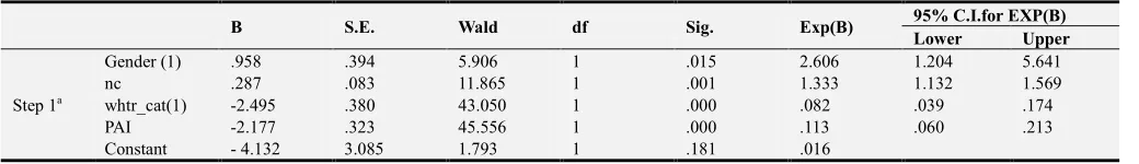
Table 11 illustrates the influence of each predictor variable to the logistic model and statistical significance (p < 0.05) of Wald Chi Square test, which is obtained by squaring the ratio of coefficient to its standard error.

Table 11. Parameter Estimates Table.

B S.E. Wald df Sig. Exp(B) 95% C.I.for EXP(B)

Lower Upper

Step 1a

Gender (1) .958 .394 5.906 1 .015 2.606 1.204 5.641

nc .287 .083 11.865 1 .001 1.333 1.132 1.569

whtr_cat(1) -2.495 .380 43.050 1 .000 .082 .039 .174

PAI -2.177 .323 45.556 1 .000 .113 .060 .213

Constant - 4.132 3.085 1.793 1 .181 .016

Wald Statistics tests the unique contribution of each independent variable, in the context of the other variables with significance values. The categorical variables gender (1) (p = 0.015), whtr_cat (p = 0.0001) and the continuous variables nc (p = 0.001) and PAI (p = 0.0001) have added significant contribution to the model.

Hence, the binary logistic regression function is given by ln(odds) = − 4.132 + 0.958 (gender ) + 0.287 (nc) – 2.495

(whtr_cat) − 2.177 (PAI). The odds prediction equation is

Odds = e (−4.132+0.958(gender)+0.287(nc)–2.495(whtr_cat)−2.177(PAI). This function can be used to predict the odds that a subject of a given gender, nc, whtr_cat and PAI will be overweight. Effect of neck circumference is smaller, with a one-unit increase on the neck circumference being associated with the odds of subjects falling in the overweight group increasing by a multiplicative factor of 1.333. Inverted odds ratios for the whtr_cat variable indicated that the odds of falling in overweight group were 12.19 times higher for the subjects classified in overweight group of waist to height ratio. Inverting the odds ratio 0.113 for physical activity index shows that for one unit increase in the PAI value there was 8.85 of the odds that the subject would not fall in the category of overweight. Female subjects are 2.6 times more likely to be overweight than males. The odds of falling in overweight group, is 0.384 times lower in male as opposed to female subjects. By converting odds to probabilities, for female, odds / (1+ odds) = 2.6/3.6 = 0.722. It means the model predicts that 72.2% of female will be in the category of no overweight and 27.8% of them will be overweight. In overweight group, 14.7% of male subjects are classified and 85.3% are grouped into no overweight.

4. Conclusion

The present study has used meaningful statistical tools to identify the association of significant variables with the overweight of the subjects. The binary logistic regression analysis was performed to determine the effects of gender, neck circumference, waist to height ratio, and physical activity index on the likelihood that subjects have overweight. The model was statistically significant based on Chi square =188.863, p < 0.0001 with d.f. 4. The model explained 55.8% (Nagelkerke R2) of the variance in the overweight and correctly classified 87.7% of cases. The odds ratio for gender indicates that when holding all other variables constant, female subjects were 2.6 times more likely to demonstrate overweight than males. The subjects classified to no overweight group based on waist to height ratio were associated with a reduction in the likelihood of falling to overweight group. The increment in the value of neck circumference was associated with an increased likelihood of falling to overweight category of subjects, but increasing physical activity index was related with a

reduction in the likelihood of falling to overweight group. Hence, the prevalence of overweight for both subjects is 22.4%. The prevalence of overweight is higher in female (27.8%) than in male (14.7%) subjects, which is consistent with the result of previous studies [2, 3]. It is very important for each individual to focus on the food intake pattern, physical activity, lifestyle, and also their physical measurements. The awareness about the importance of physical activities and measurement of neck circumference and waist to height ratio to live a healthy life should be communicated among the young students. Further research can be carried out by taking into account significant risk factors associated with the overweight of a person.

References

[1] Popkin, B. (2009). The world is fat: the fads, trends, policies, and products that are fattening the human race. USA: Penguin Group.

[2] WHO. (2013). Non-communicable disease risk factor survey Nepal 2013. Kathmandu: Nepal Health Research Council and World Health Organization.

[3] Ministry of Health, New ERA, and ICF. (2017). Nepal demographic and health survey 2016. Nepal: Ministry of Health. [4] Lahav, Y., Yoram, E., Ron, K., and Haggai, S. (2018). A novel

body circumferences based estimation of percentage body fat. British Journal of Nutrition, 119(6), 720-725.

[5] WHO. (2017). WHO country cooperation strategy Nepal 2013-2017. India: World Health Organization.

[6] Hu, F. (2008). Measurements of adiposity and body composition. In: Hu F, ed. Obesity Epidemiology, 53–83. New York: Oxford University Press.

[7] WHO. (2000). Obesity: preventing and managing the global epidemic, Geneva: World Health Organization.

[8] WHO. (2008). Waist circumference and waist-hip ratio: Report of a WHO expert consultation. Switzerland: World Health Organization.

[9] Lancet. (2004). Appropriate body-mass index for Asian populations and its implications for policy and intervention strategies. WHO expert consultation Public Health, 363(9403), 157-163.

[10] Hung, S. P., Chen, C. Y., Guo, F. R., Chang, C. I., and Jan, C. F. (2017). Combine body mass index and body fat percentage measures to improve the accuracy of obesity screening in young adults. Obesity Research and Clinical Practice, 11(1), 11-18. [11] Berrington, G. A., Hartge, P., Cerhan, J. R., et al. (2010). Body

mass index and mortality among 1.46 million white adults. New England Journal of Medicine, 363: 2211-2219.

[12] World Health Organization. (2018). What is Moderate-intensity and Vigorous-intensity Physical Activity? Available at www.who.int/dietphysicalactivity/physical_activity_intensity/en/. [13] Javier, G. A., Victor, V., et al. (2012). Clinical usefulness of a

[14] Swainson, M. G., Batterham, A. M., Tsakirides, C., Rutherford, Z. H., and Hind, K. (2017). Prediction of whole-body fat percentage and visceral adipose tissue mass from five anthropometric variables. PLoS ONE, 12(5): e0177175. [15] Ho-Pham, L. T., Campbell, L. V., and Nguyen, T. V. (2011).

More on body fat cutoff points. Mayo Clinic Proceedings, 86(6), 584. http://doi.org/10.4065/mcp.2011.0097.

[16] Li, Y., Wang, H., Wang, K., Wang, W., Dong, F., Qian, Y., … Shan, G. (2017). Optimal body fat percentage cut-off values for identifying cardiovascular risk factors in Mongolian and Han adults: a population-based cross-sectional study in Inner Mongolia, China. BMJ Open, 7(4), e014675.

[17] Belinda, B. and Peat, J. (2014). Medical statistics: a guide to SPSS, data analysis, and critical appraisal (2nd ed.). UK: Wiley.

[18] Sylvia, W. S. (2004). Biostatistics and Epidemiology: a primer for health and biomedical professional (3rd ed.). USA: Springer.

[19] Kleinbaum, G. D., and Klein, M. (2010). Logistic regression: A self learning text (3rd ed.). New York: Springer.

[20] Valeria, F. and Eduard, B. (2017). Features selection using LASSO. Research paper in Business Analytics, VU: Amsterdam.

[21] Hosmer, D. W., Hosmer, T., Le Cessie, S., and Lemeshow, S. (1997). A comparison of goodness of fit test for the logistic regression model, Statistics in Medicine, 16, 965-980. [22] Cox, D. R., and Snell, E. J. (1989). Analysis of binary data

(2nd ed.). London: Chapman and Hall.

[23] Hosmer, D. W. and Lemeshow, S. (2000). Applied logistic regression (2nd ed.). New York: John Wiley & Sons.