Learning Control Knowledge for Forward Search Planning
Sungwook Yoon [email protected]
Computer Science and Engineering Department Arizona State University
Tempe, AZ 85281
Alan Fern [email protected]
School of Electrical Engineering and Computer Science Oregon State University
Corvallis, OR 97330
Robert Givan [email protected]
School of Electrical and Computer Engineering Purdue University
West Lafayette, IN 47907
Editor: Carlos Guestrin
Abstract
A number of today’s state-of-the-art planners are based on forward state-space search. The im-pressive performance can be attributed to progress in computing domain independent heuristics that perform well across many domains. However, it is easy to find domains where such heuristics provide poor guidance, leading to planning failure. Motivated by such failures, the focus of this pa-per is to investigate mechanisms for learning domain-specific knowledge to better control forward search in a given domain. While there has been a large body of work on inductive learning of con-trol knowledge for AI planning, there is a void of work aimed at forward-state-space search. One reason for this may be that it is challenging to specify a knowledge representation for compactly representing important concepts across a wide range of domains. One of the main contributions of this work is to introduce a novel feature space for representing such control knowledge. The key idea is to define features in terms of information computed via relaxed plan extraction, which has been a major source of success for non-learning planners. This gives a new way of leverag-ing relaxed plannleverag-ing techniques in the context of learnleverag-ing. Usleverag-ing this feature space, we describe three forms of control knowledge—reactive policies (decision list rules and measures of progress) and linear heuristics—and show how to learn them and incorporate them into forward state-space search. Our empirical results show that our approaches are able to surpass state-of-the-art non-learning planners across a wide range of planning competition domains.
Keywords: planning, machine learning, knowledge representation, search
1. Introduction
is one of the oldest techniques available for planning, and many other search spaces and approaches have been developed, this state-of-the-art performance is somewhat surprising. One of the key rea-sons for the success is the development of powerful domain-independent heuristics that work well on many AI planning domains. Nevertheless, it is not hard to find domains where these heuristics do not work well, resulting in planning failure. We are motivated by these failures and in this study, we investigate machine learning techniques that find domain-specific control knowledge that can improve or speed-up forward state-space search in a non-optimal, or satisficing, planning setting.
As outlined in Section 3 there is a large body of work on learning search-control knowledge for AI planning domain. However, despite the significant effort, none of these approaches has been demonstrated to be competitive with state-of-the-art non-learning planners across a wide range of planning domains. There are at least two reasons for the performance gap between learning and non-learning planners. First, most prior work on learning control knowledge has been in the context of non-state-of-the-art planning approaches such as partial-order planning, means-ends analysis, among others. In fact, we are only aware of two recent efforts (Botea et al., 2005; Coles and Smith, 2007) that learn control knowledge for forward state-space search planners. Even these approaches have not demonstrated the ability to outperform the best non-learning planners as measured on plan-ning competition domains. Second, it is a challenge to define a hypothesis space for representing control knowledge that is both rich enough for a wide variety of planning domains, yet compact enough to support efficient and reliable learning. Indeed, a common shortcoming of much of the prior work is that the hypothesis spaces, while adequate for the small number of domains investi-gated, were not rich enough for many other domains.
The primary goal of this work is to contribute toward reversing the performance gap between learning and non-learning planners. In this work, we do this by addressing each of the above two issues. First, our system is based on the framework of forward state-space search, in particular, being built upon the state-of-the-art planner FF (Hoffmann and Nebel, 2001). Second, we propose a novel hypothesis space for representing useful heuristic features of planning states. We show how to use this feature space as a basis for defining and learning several forms of control knowledge that can be incorporated into forward state-space search. The result is a learning-based planner that learns control knowledge for a planning domain from a small number of solved problems and is competitive with and often better than state-of-the-art non-learning planners across a substantial set of benchmark domains and problems.
A key novelty of our proposed feature space is that it leverages the computation of relaxed plans, which are at the core of the computation of modern forward-search heuristics (Bonet and Geffner, 2001; Hoffmann and Nebel, 2001). Relaxed plans are constructed by ignoring, to varying degrees, the delete/negative effects of actions and can be computed very efficiently. The length of these plans can then serve as an informative heuristic (typically non-admissible) for guiding state-space search. In addition to their length, relaxed plans contain much more information about a search state that is ignored by most forward-search planners.1 Our proposed feature space gives one way of using this information by viewing the relaxed plan as a structure for defining potentially useful features of the current state. As an example of the utility of our feature space, note that the fact that relaxed planning ignores delete effects is the main reason that the length sometimes dramatically underestimates the true distance to goal, leading to poor heuristic guidance (note that relaxed-plan length can also overestimate the distance to goal). Our feature space is able to partially
capture information about the delete effects ignored in a relaxed plan, which can be used to learn knowledge that partially compensates for the underestimation.
We use the relaxed-plan feature space to learn two forms of knowledge for controlling forward state-space planning. In each case, the knowledge is learned based on a set of training problems from a domain, each labeled by a solution. First, we consider learning knowledge in the form of linear heuristic functions. In particular, we learn heuristics that are linear combinations of relaxed-plan features, with one of those features being the relaxed-relaxed-plan length. Thus, our heuristic learner can be viewed as an approach for automatically correcting deficiencies of the usual relaxed-plan length heuristic, by augmenting it with a weighted combination of additional features selected from the large space of possible relaxed-plan features.
As a second form of control knowledge, we investigate reactive policies. Learning reactive policies for planning domains has been studied by several researchers (Khardon, 1999; Martin and Geffner, 2000; Yoon et al., 2002, 2005). However, all of these studies have used the learned policies as stand-alone search-free planners that simply execute the linear sequence of actions selected by the policies. While this non-search approach is efficient and has been shown to work well in a number of domains, it often fails due to flaws in the policy that arise due to imperfect learning. Nevertheless, such policies capture substantial information about the planning domain, which we would like to exploit in a more robust way. In this work, we propose and evaluate a simple way of doing this by integrating learned policies into forward search. At each search node (i.e., state), we execute the learned policy for a fixed horizon and add all of the states encountered to the search queue. In this way, flaws in the policy can be overcome by search, while the search efficiency can be substantially improved by quickly uncovering good “deep states” that are found by the policy. We evaluate this idea using two representations for learned policies both of which make use of relaxed-plan features—decision lists of rules similar to Yoon et al. (2002) and measures of progress (Yoon et al., 2005)—both of which make use of relaxed-plan features.
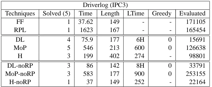
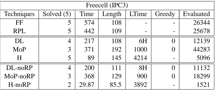
In our experiments, we learned and evaluated both forms of control knowledge on benchmark problems from recent planning competitions. We learned on the first 15 problems in each domain and tested on the remaining problems. The results are very much positive. Forward state-space search with the learned control knowledge outperforms state-of-the-art planners, in most of the competition domains. We also demonstrate the utility of our relaxed-plan feature space by con-sidering feature spaces that ignore parts of the relaxed-plan information, showing that using the relaxed-plan information leads to the best performance.
2. Problem Setup
In this paper, we focus our attention on learning control knowledge for deterministic STRIPS plan-ning domains. Below we first give a formal definition of the types of planplan-ning domains we consider and then describe the learning problem.
2.1 Planning Domains
A deterministic planning domain
D
defines a set of possible actionsA
and a set of statesS
in terms of a set of predicate symbolsP
, action types Y , and objects O. Each state inS
is a set of facts, where a fact is an application of a predicate symbol inP
to the appropriate number of objects fromO. There is an action in
A
, for each way of applying the appropriate number of objects in O to anaction type symbol in Y . Each action a∈
A
consists of: 1) an action name, which is an action type applied to the appropriate number of objects, 2) a set of precondition state facts Pre(a), 3) two sets of state facts Add(a)and Del(a)representing the add and delete effects respectively. As usual, an action a is applicable to a state s iff Pre(a)⊆s, and the application of an (applicable) action a to s,denoted a(s), results in the new state a(s) = (s\Del(a))∪Add(a).
Given a planning domain, a planning problem P from the domain is a tuple (s,A,g), where
A⊆
A
is a set of applicable actions, s∈S
is the initial state, and g is a set of state facts representing the goal. A solution plan for a planning problem is a sequence of actions(a1, . . . ,ah), where the sequential application of the sequence starting in state s leads to a goal state s0 where g⊆s0. Later in the paper, in Section 7, when discussing measures of progress, it will be useful to talk about reachability and deadlocks. We say that a planning problem (s,A,g) is reachable from problem (s0,A,g) iff there is some action sequence in A∗ that leads from s0 to s. We say that a planningproblemPis deadlock free iff all problems reachable fromPare solvable.
2.2 Learning Control Knowledge from Solved Problems
The bi-annual International Planning Competition (IPC), has played a large role in the recent progress observed in AI planning. Typically the competition is organized around a set of plan-ning domains, with each domain providing a sequence of planplan-ning problems, often in increasing order of difficulty. Despite the fact that the planners in these competitions experience many similar problems from the same domain, to our knowledge only one of them, Macro-FF (Botea et al., 2005), has made any attempt to learn from previous experience in a domain to improve performance on later problems.2 Rather they solve each problem as if it were the first time the domain had been en-countered. The ability to effectively transfer domain experience from one problem to the next would provide a tremendous advantage. Indeed, the potential benefit of learning domain-specific control knowledge can be seen by the impressive performance of planners such as TL Plan (Bacchus and Kabanza, 2000) and SHOP (Nau et al., 1999), where human-written control knowledge is provided for each domain. However, to date, most “learning to plan” systems have lagged behind the state-of-the-art non-learning domain-independent planners. One of the motivations and contributions of this work is to move toward reversing that trend.
The input to our learner will be a set of problems for a particular planning domain along with a solution plan to each problem. The solution plan might have been provided by a human or
ically computed using a domain-independent planner (for modestly sized problems). The goal is to analyze the training set to extract control knowledge that can be used to more effectively solve new problems from the domain. Ideally, the control knowledge allows for the solutions of large, difficult problems that could not be solved within a reasonable time limit before learning.
As a concrete example of this learning setup, in our experiments, we use the problem set from recent competition domains. We first use a domain-independent planner, in our case FF (Hoffmann and Nebel, 2001), to solve the low-numbered planning problems in the set (typically corresponding to the easier problems). The solutions are then used by our learner to induce control knowledge. The control knowledge is then used to solve the remaining, typically more difficult, problems in the set. Our objective here is to obtain fast, satisficing planning through learning. The whole process is domain independent, with knowledge transferring from easy to hard problems in a domain. Note that although learning times can be substantial, the learning cost can be amortized over all future problems encountered in the domain.
3. Prior Work
There has been a long history of work on learning-to-plan, originating at least back to the original STRIPS planner (Fikes et al., 1972), which learned triangle tables or macros that could later be exploited by the planner. For a collection and survey of work on learning in AI planning see Minton (1993) and Zimmerman and Kambhampati (2003).
A number of learning-to-plan systems have been based on the explanation-based learning (EBL) paradigm, for example, Minton et al. (1989) among many others. EBL is a deductive learning approach, in the sense that the learned knowledge is provably correct. Despite the relatively large effort invested in EBL research, the best approaches typically did not consistently lead to significant gains, and even hurt performance in many cases. A primary way that EBL can hurt performance is by learning too many, overly specific control rules, which results in the planner spending too much time simply evaluating the rules at the cost of reducing the number of search nodes considered. This problem is commonly referred to as the EBL utility problem (Minton, 1988).
Partly in response to the difficulties associated with EBL-based approaches, there have been a number of systems based on inductive learning, perhaps combined with EBL. The inductive ap-proach involves applying statistical learning mechanisms in order to find common patterns that can distinguish between good and bad search decisions. Unlike EBL, the learned control knowledge does not have guarantees of correctness, however, the knowledge is typically more general and hence more effective in practice. Some representative examples of such systems include learning for partial-order planning (Estlin and Mooney, 1996), learning for planning as satisfiability (Huang et al., 2000), and learning for the Prodigy means-ends framework (Aler et al., 2002). While these systems typically showed better scalability than their EBL counterparts, the evaluations were typi-cally conducted on only a small number of planning domains and/or small number of test problems. There is no empirical evidence that such systems are robust enough to compete against state-of-the-art non-learning planners across a wide range of domains.
its simplicity, this approach has demonstrated considerable success. However, these approaches have still not demonstrated the robustness necessary to outperform state-of-the-art non-learning planners across a wide range of domains.
Ideas from reinforcement learning have also been applied to learn control policies in AI planning domains. Relational reinforcement learning (RRL) (Dzeroski et al., 2001), used Q-learning with a relational function approximator, and demonstrated good empirical results in the Blocksworld. The Blocksworld problems they considered were complex from a traditional RL perspective due to the large state and action spaces, however, they were relatively simple from an AI planning perspective. This approach has not yet shown scalability to the large problems routinely tackled by today’s planners. A related approach, used a more powerful form of reinforcement learning, known as approximate policy iteration, and demonstrated good results in a number of planning competition domains (Fern et al., 2006). Still the approach failed badly on a number of domains and overall does not yet appear to be competitive with state-of-the-art planners on a full set of competition benchmarks.
The most closely related approaches to ours are recent systems for learning in the context of forward state-space search. Macro-FF (Botea et al., 2005) and Marvin (Coles and Smith, 2007) learn macro action sequences that can then be used during forward search. Macro-FF learns macros from a set of training problems and then applies them to new problems. Rather, Marvin is an online learner in the sense that it acquires macros during search in a specific problem that are applied at later stages in the search. As evidenced in the recent planning competitions, however, neither system dominates the best non-learning planners.
Finally, we note that researchers have also investigated domain-analysis techniques, for exam-ple, Gerevini and Schubert (2000) and Fox and Long (1998), which attempt to uncover structure in the domain by analyzing the domain definition. These approaches have not yet demonstrated the ability to improve planning performance across a range of domains.
4. Control Knowledge for Forward State-Space Search
In this section, we describe the two general forms of control knowledge that we will study in this work: heuristic functions and reactive policies. For each, we describe how we will incorporate them into forward state-space search in order to improve planning performance. Later in the paper, in Sections 6 and 7, we will describe specific representations for heuristics and policies and give algorithms for learning them from training data.
4.1 Heuristic Functions
The first and most traditional forms of control knowledge we consider are heuristic functions. A heuristic function H(s,A,g)is simply a function of a state s, action set A, and goal g that estimates the cost of achieving the goal from s using actions in A. If a heuristic is accurate enough, then greedy application of the heuristic will find the goal without search. However, when a heuristic is less accurate, it must be used in the context of a search procedure such as best-first search, where the accuracy of the heuristic impacts the search efficiency. In our experiments, we will use best-first search, which has often been demonstrated to be an effective, though sub-optimal, search strategy in forward state-space planning. Note that by best-first search, here we mean a search that is guided by only the heuristic value, rather than the path-cost plus heuristic value. This search is also called
best-first search and we will add greedy in front of best-best-first search to remind the readers, as necessary, in the following texts.
Recent progress in the development of domain-independent heuristic functions for planning has led to a new generation of state-of-the-art planners based on forward state-space heuristic search (Bonet and Geffner, 2001; Hoffmann and Nebel, 2001; Nguyen et al., 2002). However, in many domains these heuristics can still have low accuracy, for example, significantly underestimating the distance to goal, resulting in poor guidance during search. In this study, we will attempt to find regular pattern of heuristic inaccuracy (either due to over or under estimation) through machine learning and compensate the heuristic function accordingly.
We will focus our attention on linear heuristics that are represented as weighted linear combi-nations of features, that is, H(s,A,g) =Σiwi·fi(s,A,g), where the wi are weights and the fi are functions. In particular, for each domain we would like to learn a distinct set of features and their corresponding weights that lead to good planning performance in that domain. Note that some of the feature functions can correspond to existing domain-independent heuristics, allowing for our learned heuristics to exploit the useful information they already provide, while overcoming defi-ciencies by including additional features. The representation that we use for features is discussed in Section 5 and our approach to learning linear heuristics over those features is described in Section 6.
In all of our experiments, we use the learned heuristics to guide (greedy) best-first search when solving new problems.
4.2 Reactive Policies in Forward Search
The second general form of control knowledge that we consider in this study is of reactive policies. A reactive policy is a computationally efficient functionπ(s,A,g), possibly stochastic, that maps a planning problem(s,A,g)to an action in A. Given an initial problem(s0,A,g), we can use a reac-tive policyπto generate atrajectory of pairs of problems and actions(((s0,A,g),a0),((s1,A,g),a1), ((s2,A,g),a2). . .), where ai=π(si,A,g)and si+1=ai(si). Ideally, given an optimal or near-optimal policy for a planning domain, the trajectories represent high-quality solution plans. In this sense, re-active policies can be viewed as efficient domain-specific planners that avoid unconstrained search. Later in the paper, in Section 7, we will introduce two formal representations for policies: decision rule lists and measures of progress, and describe learning algorithms for each representation. Below we describe some of the prior approaches to using policies to guide forward search and the new approach that we propose in this work.
The simplest approach to using a reactive policy as control knowledge is to simply avoid search altogether and follow the trajectory suggested by the policy. There have been a number of studies (Khardon, 1999; Martin and Geffner, 2000; Yoon et al., 2002, 2005; Fern et al., 2006) that consider using learned policies in this way in AI planning context. While there have been some positive results, for many planning domains the results have been mostly negative. One reason for these failures is that inductive, or statistical, policy learning can result in imperfect policies, particularly with limited training data. Although these policies may select good actions in many states, the lack of search prevents them from overcoming the potentially numerous bad action choices.
rollout (Bertsekas and Tsitsiklis, 1996). Unfortunately, our initial investigation showed that in many planning competition domains these techniques were not powerful enough to overcome the flaws in our learned polices. With this motivation we developed a novel approach that is easy to implement and has proven to be quite powerful.
The main idea is to use reactive policies during the node expansion process of a heuristic search, which in our work is greedy best-first search. Typically in best-first search, only the successors of the current node being expanded are added to the priority queue, where priority is measured by heuristic value. Rather, our approach first executes the reactive policy for h steps from the node being expanded and adds the nodes of the trajectory along with their neighbors to the queue. In all of our experiments, we used a value of h=50, though we found that the results were quite stable across a range of h (we sampled a range from 30 to 200).
Note that when h=0 we get standard (greedy) best-first search. In cases, where the policy can solve a given problem from the current node being expanded, this approach will solve the problem without further search provided that h is large enough. Otherwise, when the policy does not directly lead to the goal, it may still help the search process by putting heuristically better nodes in the search queue in a single node expansion. Without the policy (i.e., h=0) such nodes would only appear in the queue after many node expansions. Intuitively, given a reasonably good heuristic, this approach is able to leverage the good choices made by a policy, while overcoming the flaws. While this technique for incorporating policies into search is simple, our empirical results, show that it is very effective, achieving better performance than either pure heuristic search or search-free policy execution.
5. A Relaxed-Plan Feature Space
A key challenge toward learning control knowledge in the form of heuristics and policies is to develop specific representations that are rich enough to capture important properties of search nodes. In this section, we describe a novel feature space for representing such properties. This feature space will be used as a basis for our policy and heuristic representations described in Sections 6 and 7. Note that throughout, for notational convenience we will describe each search node by its implicit planning problem(s,A,g), where s is the current state of the node, g is the goal, and A is the action
set.
Each feature in our space is represented via an expression in taxonomic syntax, which as de-scribed in Section 5.4, provides a language for describing sets of objects with common properties. Given a search node(s,A,g)and a taxonomic expression C, the value of the corresponding feature is computed as follows. First, a database of atomic facts D(s,A,g) is constructed, as described in Section 5.3, which specifies basic properties of the search node. Next, we evaluate the class expres-sion C relative to D(s,A,g), resulting in a class or set of objects. These sets, or features, can then be used as a basis for constructing control knowledge in various ways—for example, using the set cardinalities to define a numeric feature representation of search nodes.
Our feature space, is in the spirit of prior work (Martin and Geffner, 2000; Yoon et al., 2002; Fern et al., 2006) that also used taxonomic syntax to represent control knowledge. However, our ap-proach is novel in that we construct databases D(s,A,g)that contain not only facts about the current
defining features in terms of taxonomic expressions built from our extended databases, we are able to capture properties that are difficult to represent in terms of the state and goal predicates alone.
In the remainder of this section, we first review the idea of relaxed planning, which is central to our feature space. Next, we describe the construction of the database D(s,A,g)for search nodes. Finally, we introduce taxonomic syntax, which is used to build complex features on top of the database.
5.1 Relaxed Plans
Given a planning problem (s,A,g), we define the corresponding relaxed planning problem to be the problem(s,A+,g)where the new action set A+is created by copying A and then removing the
delete list from each of the actions. Thus, a relaxed planning problem is a version of the original planning problem where it is not necessary to worry about delete effects of actions. A relaxed plan for a planning problem(s,A,g)is simply a plan that solves the relaxed planning problem.
Relaxed planning problems have two important characteristics. First, although a relaxed plan may not necessarily solve the original planning problem, the length of the shortest relaxed plan serves as an admissible heuristic for the original planning problem. This is because preconditions and goals are defined in terms of positive state facts, and hence removing delete lists can only make it easier to achieve the goal. Second, in general, it is computationally easier to find relaxed plans compared to solving general planning problems. In the worst case, this is apparent by noting that the problem of plan existence can be solved in polynomial time for relaxed planning problems, but is PSPACE-complete for general problems. However, it is still NP-hard to find minimum-length relaxed plans (Bylander, 1994). Nevertheless, practically speaking, there are very fast polynomial time algorithms that typically return short relaxed plans whenever they exist, and the lengths of these plans, while not admissible, often provide good heuristics.
The above observations have been used to realize a number of state-of-the-art planners based on heuristic search. HSP (Bonet and Geffner, 2001) uses forward state-space search guided by an admissible heuristic that estimates the length of the optimal relaxed plan. FF (Hoffmann and Nebel, 2001) also takes this approach, but unlike HSP, estimates the optimal relaxed-plan length by explicitly computing a relaxed plan. FF’s style of relaxed plan computation is linear with the length of the relaxed plan, thus fast, but the resulting heuristics can be inadmissible. Our work builds on FF, using the same relaxed-plan construction technique, which we briefly describe below.
While the length of FF’s relaxed plan often serves as an effective heuristic, for a number of planning domains, ignoring delete effects leads to severe underestimates of the distance to a goal. The result is poor guidance and failure on all but the smallest problems. One way to overcome this problem would be to incorporate partial information about delete lists into relaxed plan computation, for example, by considering mutex relations. However, to date, this has not born out as a practical alternative. Another possibility is to use more information about the relaxed plan than just its length. For example, Vidal (2004) uses relaxed plans to construct macro actions, which help the planner overcome regions of the state space where the relaxed-plan length heuristic is flat. However, that work still uses length as the sole heuristic value. In this work, we give a novel approach to leveraging relaxed planning, in particular, we use relaxed plans as a source of information from which we can compute complex features that will be used to learn heuristic functions and policies. Interestingly, as we will see, this approach will allow for features that are sensitive to delete lists of actions in relaxed plans, which can be used to help correct for the fact that relaxed plans ignore delete effects.
A
B
C
A
B
C
Init State
Goal
A
B
C
A
B
C
S
1S
2on( A, B) on(A, table)
on(B, table) on( C, table)
holding(A) holding(B) clear(A) clear(B) clear( C) on(B, C) pickup(A) pickup(B) stack(A,B) stack(B,C) on(B, table) on( C, table)
holding(B)
clear(A)
on(B, C) unstack(A,B) pickup(B) stack(B,C)
clear( C) on(A, B)
clear(B)
Del{ on(A,B)}
Level 1 Level 2 Level 3 Level 4 Level 5
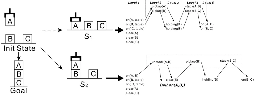
Figure 1: Blocksworld Example
5.2 Example of using Relaxed Plan Features for Learning Heuristics
As an example of how relaxed plans can be used to define useful features, consider a problem from the Blocksworld in Figure 1. Here, we show two states S1and S2that can be reached from the initial
state by applying the actions putdown(A) and stack(A,B)respectively. From each of these states we show the optimal relaxed plans for achieving the goal. For these states, the relaxed-plan length heuristic is 3 for S2and 4 for S1, suggesting that S2is the better state. However, it is clear that, in
fact, S1is better.
Notice that in the relaxed plan for S2, on(A,B) is in the delete list of the action unstack(A,B)
and at the same time it is a goal fact. One can improve the heuristic estimation by adding together the relaxed-plan length and a term related to such deleted facts. In particular, suppose that we had a feature that computed the number of such “on” facts that were both in the delete list of some relaxed plan action and in the goal, giving a value of 0 for S1and 1 for S2. We could then weight this feature
feature as the cardinality of a certain class expression over a database of facts defined in the next section.
While this is an over-simplified example, it is suggestive as to the utility of features derived from relaxed plans. Below we describe a domain-independent feature space that can be instantiated for any planning domain. Our experiments show that these features are useful across a range of domains used in planning competitions.
5.3 Constructing Databases from Search Nodes
Recall that each feature in our feature space corresponds to a taxonomic syntax expression (see next section) built from the predicate symbols in databases of facts constructed for each search node encountered. We will denote the database for search node(s,A,g)as D(s,A,g), which will simply contain a set of ground facts over some set of predicate symbols and objects derived from the search node. Whereas prior work defined D(s,A,g) to include only facts about the goal g and state s,
we will also include facts about the relaxed plan corresponding to problem (s,A,g), denoted by (a1, . . . ,an). Note that in this work we use the relaxed plan computed by FF’s heuristic calculation. Given any search node (s,A,g)we now define D(s,A,g) to be the database that contains the
following facts:
• All of the state facts in s.
• The name of each action aiin the relaxed plan. Recall that each name is an action type Y from domain definition
D
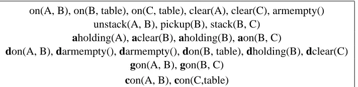
applied to the appropriate number of objects, for example, unstack(A,B).• For each state fact in the add list of some action ai in the relaxed plan, add a fact to the database that is the result of prepending an a to the fact’s predicate symbol. For example, in Figure 1, for state S2the fact holding(B)is in the add list of pickup(B), and thus we would
add the fact aholding(B)to the database.
• Likewise for each state fact in the delete list of some ai, we prepend a d to the predicate symbol and add the resulting fact to the database. For example, in Figure 1, for S2, we would
add the fact don(A,B).
• For each state fact in the goal g, we prepend a g to the predicate symbol and add it to the database. For example, in Figure 1, we would add the facts gon(A,B)and gon(B,C).
• For each predicate symbol that appears in the goal, we prepend a c to the predicate symbol and add a corresponding fact to the database whenever it is true in the current state s and appears in the goal. For example, the predicate con represents the relation “correctly on”, and in Figure 1, for state S2we would add the fact con(A,B) since A is currently on B and is
supposed to be on B in the goal. The ’c’ predicates provide a useful mechanism for expressing concepts that relate the current state to the goal.
Figure 2, shows an example of the database that would be constructed for the state S2in Figure
on(A, B), on(B, table), on(C, table), clear(A), clear(C), armempty() unstack(A, B), pickup(B), stack(B, C)
aholding(A), aclear(B), aholding(B), aon(B, C)
don(A, B), darmempty(), darmempty(), don(B, table), dholding(B), dclear(C) gon(A, B), gon(B, C)
con(A, B), con(C,table)
Figure 2: Database for state S2in Figure 1
’c’ predicates. It captures information about the relaxed plan using the action type predicates and the ’a’ and ’d’ predicates. Notice that the database does not capture information about the temporal structure of the relaxed plan. Such temporal information may be useful for describing features, and is a natural extension of this work.
5.4 Defining Complex Features with Taxonomic Syntax
For a given search node (s,A,g) with database D(s,A,g) we now wish to define more complex features of the search node. We will do this using taxonomic syntax (McAllester and Givan, 1993) which is a first-order language for writing class expressions C that are used to denote sets of objects. In particular, given a class expression C, the set of objects it represents relative to D(s,A,g)will be denoted by C[D(s,A,g)]. Thus, each C can be viewed as defining a feature that for search node
(s,A,g)takes the value C[D(s,A,g)]. Below we describe the syntax and semantics of the taxonomic syntax fragment we use in this paper.
Syntax. Taxonomic class expression are built from a set of predicates
P
, where n(P)will be used to denote the arity of predicate P. For example, in our application the set of predicates will include all predicates used to specify facts in database D(s,A,g) as described above. The set of possible class expressions overP
are given by the following grammar:C :=a-thing|P1|C∩C| ¬C|(P C1. . .Ci−1 ? Ci+1. . .Cn(P))
where C and Cj are class expressions, P1 is any arity one predicate, and P is any predicate
sym-bol of arity two or greater. Given this syntax we see that the primitive class expressions are the special symbol a-thing, which will be used to denote the set of all objects, and single arity predi-cates, which will be used to denote the sets of objects for which the predicates are true. One can then obtain compound class expressions via complementation, intersection, or relational composi-tion (the final rule). Before defining the formal semantics of class expressions, we introduce the concept of depth, which will be used in our learning procedures. We define the depth of a class expression C, denoted depth(C) as follows. The depth of a-thing or a single arity predicate is 0, depth(C1∩C2) =1+max(depth(C1),depth(C2)), depth(¬C) =1+depth(C), and the depth of the
expression(P C1. . .Ci−1 ? Ci+1. . .Cn(P)), is 1+max depth(C1), . . . ,depth(Cn(P))
. Note that the number of class expressions can be infinite. However, we can limit the number of class expressions under consideration by placing an upper bound on the allowed depth, which we will often do when learning.
objects. For example, D might correspond to one of the databases described in the previous section. One can simply view the database D as a finite first-order model, or Herbrand interpretation. Given a class expression C and a database D, we use C[D]to denote the set of objects represented by C with respect to D. We also use P[D]to denote the set of tuples of objects corresponding to predicate
P in D, that is, the tuples that make P true.
If C=a-thing then C[D]denotes the set of all objects in D. For example, in a database con-structed from a Blocksworld state, a-thing would correspond to the set of all blocks. If C is a single arity predicate symbol P, then C[D] is the set of all objects in D for which P is true. For example, if D again corresponds to the Blocksworld then clear[D]and ontable[D]denote the sets of blocks that are clear and on the table respectively in D. If C=C1∩C2 then C[D] = C1[D]∩C2[D]. For example, (clear∩ontable)[D] denotes the set of blocks that are clear and on the table. If C=¬C0 then C[D] = a-thing−C0[D]. Finally, for relational composition, if
C= (P C1. . .Ci−1 ? Ci+1. . .Cn(P)) then C[D]is the set of all constants c such that there exists cj ∈Cj[D] such that the tuple(c1, . . . ,ci−1,c,ci+1, . . . ,cn(R)) is in P[D]. For example, if D again contains facts about a Blocksworld problem,(on clear ?)[D]is the set of all blocks that are directly under some clear block.
As some additional Blocksworld examples, C= (con a-thing ?)describes the blocks that are currently directly under the block that they are supposed to be under in the goal. So if D corresponds to the database in Figure 2 then C[D] ={B,table}. Recall that as described in the previous section
the predicate con is true of block pairs(x,y)that are correctly on each other, that is, x is currently on y and x should be on y in the goal. Likewise(con ? a-thing)is the set of blocks that are directly above the block they are supposed to be on in the goal and would be interpreted as the set{A,C}in database D. Another useful concept is¬(con ? a-thing)which denotes the set of blocks that are not currently on their final destination block and would be interpreted as{B,table}with respect to
D.
6. Learning Heuristic Functions
Given the relaxed plan feature space, we will now describe how to use that space to represent and learn heuristic functions for use as control knowledge in forward state-space search. Recall from Section 4.1 that we will use the learned heuristics to control (greedy) best-first search in our experiments. Below we first review our heuristic representation followed by a description of our learning algorithm. Recall that heuristic functions are just one of two general forms of control knowledge that we consider in this paper. Our second form, reactive policies, will be covered in the next section.
6.1 Heuristic Function Representation
search node (s,A,g) to be the cardinality of Ci with respect to D(s,A,g)—that is, fCi(s,A,g) =
|Ci[D(s,A,g)]|.
6.2 Heuristic Function Learning
The input to our learning algorithm is a set of planning problems, each paired with an example solution plan, taken from a target planning domain. We do not assume that these solutions are optimal, though there is an implicit assumption that the solutions are reasonably good. Our learning objective is to learn a heuristic function that closely approximates the observed distance-to-goal for each state in the training solutions. To do this, we first create a derived training setJthat contains a training example for each state in the solution set. In particular, for each training problem(s0,A,g)
and corresponding solution trajectory(s0,s1, . . . ,sn)we add toJa set of n examples{((si,A,g),n−
i)|i=0, . . . ,n−1}, each example being a pair of a planning problem and the observed
distance-to-goal in the training trajectory. Given the derived training setJ, we then attempt to learn a real valued function∆(s,A,g)that closely approximates the difference between the distances recorded inJand the value of FF’s relaxed-plan length (RPL) heuristic, RPL(s,A,g). We then take the final heuristic function to be H(s,A,g) =RPL(s,A,g) +∆(s,A,g).
We represent∆(s,A,g)as a finite linear combination of functions fCi with the Ci selected from
the relaxed plan feature space, that is,∆(s,A,g) =Σiwi·fCi(s,A,g). Note that the overall
represen-tation for H(s,A,g)is a linear combination of features, where the feature weight of RPL(s,A,g)has been clamped to one. Another design choice could have been to allow the weight of the RPL feature to also be learned, however, an initial exploration showed that constraining the value to be one and learning the residual∆(s,A,g)gives moderately better performance in some domains.
Learning the above representation involves selecting a set of class expressions from the above infinite space defined in Section 5 and then assigning weights to the corresponding features. One approach to this problem would be to impose a depth bound on class expressions and then learn the weights (e.g., using least squares) for a linear combination that involves all features whose depths of class expression are within the bound. However, the number of such features is exponential in the depth bound, making this approach impractical for all but very small bounds. Such an approach will also have no chance of finding important features beyond the fixed depth bound. In addition, we would prefer to use the smallest possible number of features, since the time complexity of evaluating the learned heuristic grows in proportion to the number of selected features. Thus, we consider a greedy learning approach where we heuristically search through the space of features, without imposing apriori depth bounds. The procedure described below is a relatively generic approach that we found to work well, however, alternative more sophisticated search approaches are an important direction for future work.
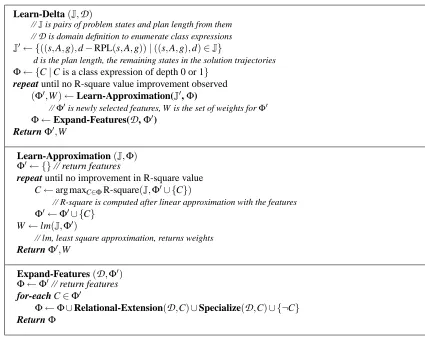
Figure 3 gives our algorithm for learning ∆(s,A,g) from a derived training set J. The main
procedure Learn-Delta first creates a modified training setJ0 that is identical to Jexcept that the
goal of each training example is changed to the difference between the distance-to-goal and FF’s relaxed-plan length heuristic. Each iteration of Learn-Delta maintains a set of class expressionsΦ, which represents the set of features that are currently under consideration. Initially
as seeds and then calling the procedure Expand-Features. This results in a larger candidate feature set, including the seed features, which is again used by Learn-Approximation to find a possibly improved approximation. We continue alternating between feature space expansion and learning an approximation until the approximation accuracy does not improve. Here we measure the accuracy of the approximation by the R-square value, which is the fraction of the variance in the data that is explained by the linear approximation.
Learn-Approximation uses a simple greedy procedure. Starting with an empty feature set, on each iteration the feature fromΦthat can most improve the R-square value of the current feature set is included in the approximation. This continues until the R-square value can no longer be improved. Given a current feature set, the quality of a newly considered feature is measured by calling the function lm from the statistics tool R, which outputs the R-square value and weights for a linear approximation that includes the new feature. After observing no improvement, the procedure returns the most recent set of selected features along with their weights, yielding a linear approximation of∆(s,A,g).
The procedure Expand-Features creates a new set of class expressions that includes the seed set, along with new expressions generated from the seeds. There are many possible ways to generate an expanded set of features from a given seed C. Here we consider three such expansion functions that worked well in practice. The first function Relational-Extension takes a seed expression C and returns all expressions of the form(P c0. . .cj−1 C cj+1. . .ci−1 ? ci+1. . .cn(P)), where P is a pred-icate symbol of arity larger than one, the ciare all a-thing, and i,j≤n(P). The result is all possible ways of constraining a single argument of a predicate by C and placing no other constraints on the predicate. For example in Blocksworld, a relational extension of the class expression, holding, is (gon holding ?). The extended expression describes the block in the goal state that should be under the block currently being held.
The second procedure for generating new expressions given a class expression C is Specialize. This procedure simply generates all class expressions that can be created by replacing a single depth zero or one sub-expression c0 of C with the intersection of c0 and another depth zero or one class expression. Note that all expressions that are produced by Specialize will be subsumed by C. That is, for any such expression C0, we have that for any database D, C0[D]⊆C[D]. As an example, given the Blocksworld expression (on ? a-thing), one of the class expression generated by Specialize would be (on ? (a-thing∩gclear)). The input class expression describes all the blocks on some block, and the example output class expression describes the blocks that are currently on blocks that should be clear in the goal state. Finally, we add the complement of the seed classes into the expanded feature set. For example in Logisticsworld, for the input class expression (cin ? a-thing), the complement output is ¬(cin ? a-thing). The input describes packages that are already in the goal location, and the output describes packages that are not in the goal location.
7. Learning Reactive Policies
Learn-Delta(J,D)
//Jis pairs of problem states and plan length from them
//Dis domain definition to enumerate class expressions
J0← {((s,A,g),d−RPL(s,A,g))|((s,A,g),d)∈J}
d is the plan length, the remaining states in the solution trajectories
Φ← {C|C is a class expression of depth 0 or 1} repeat until no R-square value improvement observed
(Φ0,W)←Learn-Approximation(J0,Φ)
//Φ0is newly selected features, W is the set of weights forΦ0
Φ←Expand-Features(D,Φ0) ReturnΦ0,W
Learn-Approximation(J,Φ) Φ0← {}// return features
repeat until no improvement in R-square value C←arg maxC∈ΦR-square(J,Φ0∪ {C})
// R-square is computed after linear approximation with the features
Φ0←Φ0∪ {C}
W ←lm(J,Φ0)
// lm, least square approximation, returns weights
ReturnΦ0,W
Expand-Features(D,Φ0) Φ←Φ0// return features
for-each C∈Φ0
Φ←Φ∪Relational-Extension(D,C)∪Specialize(D,C)∪ {¬C} ReturnΦ
Figure 3: Pseudo-code for learning heuristics: The learning algorithm used to approximate the dif-ference between the relaxed plan length heuristic and the observed plan lengths in the training data.
7.1 Taxonomic Decision Lists
We first consider representing and learning policies as taxonomic decision lists. Similar representa-tions have been considered previously (Martin and Geffner, 2000; Yoon et al., 2002), though this is the first work that builds such lists from relaxed-plan-based features.
7.1.1 REPRESENTATION
A taxonomic decision list policy is a list of taxonomicaction-selection rules. Each rule has the form
a(x1, . . . ,xk): L1,L2, . . .Lm
where a is a k-argument action type, the Li areliterals, and the xi are action-argument variables. Each literal has the form x∈C, where C is a taxonomic syntax class expression and x is an
Given a search node(s,A,g)and a list of action-argument objects O= (o1, . . . ,ok), we say that a literal xi∈C is satisfied if oi∈C[D(s,A,g)], that is, object oisatisfies the constraint imposed by the class expression C. We say that a rule R=a(x1, . . . ,xk): L1,L2, . . .Lmsuggests action a(o1, . . .ok) in(s,A,g)if each literal in the rule is true given(s,A,g)and O, and the preconditions of the action are satisfied in s. Note that if there are no literals in a rule for action type a, then all legal actions of type a are suggested by the rule. A rule can be viewed as placing mutual constraints on the tuples of objects that an action type can be applied to. Note that a single rule may suggest no action or many actions of one type. Given a decision list of such rules we say that an action is suggested by the list if it is suggested by some rule in the list, and no previous rule suggests any actions. Again, a decision list may suggest no action or multiple actions of one type.
A decision list L defines a deterministic policy π[L]as follows. If L suggests no action for
node(s,A,g), thenπ[L](s,A,g)is the lexicographically least action in s, whose preconditions are satisfied; otherwise, π[L](s,A,g) is the least action suggested by L. It is important to note that
sinceπ[L]only considers legal actions, as specified by action preconditions, the rules do not need
to explicitly encode the preconditions, which allows for simpler rules and learning. In other words, we can think of each rule as implicitly containing the preconditions of its action type.
As an example of a taxonomic decision list policy, consider a simple Blocksworld domain where the goal is to place all of the blocks on the table. The following policy will solve any problem in the domain.
putdown(x1) : x1∈holding,
pickup(x1) : x1∈(on ? (on ? a-thing)).
The first rule will cause the agent to putdown any block that is being held. Otherwise, if no block is being held, then the second rule will pickup a block x1 that is directly on top of a block that is
directly on top of another object (either the table or another block). In particular, this will pickup a block at the top of a tower of height two or more, as desired.3
7.1.2 DECISIONLISTLEARNING
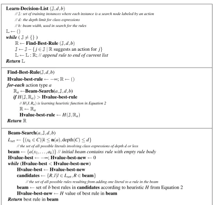
Figure 4 depicts the learning algorithm we use for decision list policies. The training setJpassed to the main procedure Learn-Decision-List is a multi-set that contains all pairs of search nodes and corresponding actions observed in the solution trajectories. The objective of the learning algo-rithm is to find a taxonomic decision list that for each search node in the training set suggests the corresponding action.
The algorithm takes a Rivest-style decision list learning approach (Rivest, 1987) where one rule is learned at a time, from highest to lowest priority, until the resulting rule set “covers” all of the training data. Here we say that a rule covers a training example if it suggests an action for the corresponding state. An ideal rule is one that suggests only actions that are in the training data.
The main procedure Learn-Decision-List initializes the rule list to()and then calls the proce-dure Find-Best-Rule in order to select a rule that covers many training examples and that correctly covers a high fraction of those examples—that is, a rule with high coverage and high precision. The resulting rule is then added to the tail of the current decision list, and at the same time the training examples that it covers are removed from the training set. The procedure then searches for another
3. If the second rule is changed to pickup(x1): x1∈(on ? a-thing), then the decision rule list may find the loop, since
Learn-Decision-List(J,d,b)
//J: set of training instances where each instance is a search node labeled by an action // d: the depth limit for class expressions
// b: beam width, used in search for the rules
L←()
while (J6={})
R←Find-Best-Rule(J,d,b)
J←J− {j∈J|Rsuggests an action for j} L←L:R; // append rule to end of current list
ReturnL
Find-Best-Rule(J,d,b)
Hvalue-best-rule← −∞;R←()
for-each action type a
Ra←Beam-Search(a,J,d,b) if H(J,Ra)>Hvalue-best-rule
// H(J,Ra)is learning heuristic function in Equation 2
R←Ra
Hvalue-best-rule←H(J,Ra)
ReturnR
Beam-Search(a,J,d,b)
Lset← {(xk∈C)|k≤n(a),depth(C)≤d}
// the set of all possible literals involving class expressions of depth d or less
beam← {a(x1, . . . ,ak)}// initial beam contains rule with empty rule body
Hvalue-best← −∞; Hvalue-best-new←0
while (Hvalue-best<Hvalue-best-new) Hvalue-best←Hvalue-best-new candidates← {R,l|l∈Lset,R∈beam}
// the set of all possible rules resulting from adding one literal to a rule in the beam
beam←set of b best rules in candidates according to heuristic H from Equation 2
Hvalue-best-new←H value of best rule in beam Return best rule in beam
Figure 4: Pseudo-code for learning policy
rule with high coverage and high precision with respect to the reduced training set. The process of selecting good rules and reducing the training set continues until no training examples remain uncovered. Note that by removing the training examples covered by previous rules we force Find-Best-Rule to focus on only the training examples for which the current rule set does not suggest an action.
The key procedure in the algorithm is Find-Best-Rule, which at each iteration does a search through the exponentially large rule space for a good rule. Recall that each rule has the form
a(x1, . . . ,xk): L1,L2, . . .Lm
loops over each action type a and then uses a beam search to construct a set of literals for that par-ticular a. The best of these rules, as measured by an evaluation heuristic, is then returned. It remains to describe the beam search over literal sets and our heuristic evaluation function.
The input to the procedure Beam-Search is the action type a, the current training set, a beam width b, and a depth bound d on the maximum size of class expressions that will be considered. The beam width and the depth bound are user specified parameters that bound the amount of search. We used d=2,b=10 in all of our experiments. The search is initialized so that the current beam contains only the empty rule, that is, a rule with head a(x1, . . . ,xk)and no literals. On each iteration of the search a candidate rule set is constructed that contains one rule for each way of adding a new literal, with depth bound d, to one of the rules in the beam. If there are n possible literals of depth bound d this will resulting in a set of nb rules. Next the rule evaluation heuristic is used to select the best b of these rules which are kept in the beam for the next iteration, with all other candidates being discarded. The search continues until the search is unable to uncover an improved rule as measured by the heuristic.
Finally, our rule evaluation heuristic H(J,R)is shown in Equation 2, which evaluates a rule R
with respect to a training set J. There are many good choices for heuristics and this is just one
that has shown good empirical performance in our experience. Intuitively this function will prefer rules that suggest correct actions for many search nodes in the training set, while at the same time minimizing the number of suggested actions that are not in the training data. We use R(s,A,g)to represent the set of actions suggested by rule R in (s,A,g). Using this, Equation 1, evaluates the “benefit” of rule R on training instance ((s,A,g),a) as follows. If the training set action a is not
suggested by R then the benefit is zero. Otherwise the benefit decreases with the size of R(s,A,g). That is, the benefit decreases inversely with the number of actions other than a that are suggested. The overall heuristic H is simply the sum of the benefits across all training instances. In this way the heuristic will assign small heuristic values to rules that cover only a small number of examples and rules that cover many examples but suggest many actions outside of the training set.
benefit(((s,A,g),a),R) = (
0 : a6∈R(s,A,g) 1
|R(s,A,g)| : a∈R(s,A,g),
(1)
H(J,R) =
∑
j∈J
benefit(j,R). (2)
7.2 Measures of Progress
In this section, we describe the notion of measures of progress and how they can be used to define policies and learned from training data.
7.2.1 REPRESENTATION
Good trajectories also often exhibit locally monotonic properties: properties that increase mono-tonically for identifiable local periods, but not all the time during the trajectory. For example, in Blocksworld, consider a block “solvable” if its desired destination is clear and well placed from the table up. Then, in good trajectories, while the number of blocks well placed from the table up stays the same, the number of solvable blocks need never decrease locally; but, globally, the number of solvable blocks may decrease as the number of blocks well placed from the table up increases. Sequences of such properties can be used to define policies that select actions in order to improve the highest-priority property possible, while preserving higher-priority properties.
Previously, the idea of monotonic properties of planning domains have been identified by Parmar (2002) as “measures of progress” and we inherit the term and expand the idea to ensembles of measures where the monotonicity is provided via a prioritized list of functions. Let F= (F1, . . . ,Fn) be an ordered list where each Fi is a function from search nodes to integers. Given an F we define an ordering relation on search nodes(s,A,g)and(s0,A,g)as F(s,A,g)F(s0,A,g)if Fi(s,A,g)> Fi(s0,A,g)while Fj(s,A,g) =Fj(s0,A,g)for all j<i. F is a strong measure of progress for planning domain
D
iff for any reachable problem(s,A,g)ofD
, either g⊆s or there exists an action a suchthat F(a(s),A,g)F(s,A,g). This definition requires that for any state not satisfying the goal there
must be an action that increases some component heuristic Fi while maintaining the preceding, higher-priority components. In this case we say that such an action has priority i. Note that we allow the lower priority heuristics that follow Fi to decrease so long as Fi increases. If an action is not able to increase some Fi, while maintaining all higher-priority components, we say that the action has null priority. In this work we represent our prioritized lists of functions F= (F1, . . . ,Fn) using a sequence of class expressions C= (C1, . . . ,Cn) and just as was the case for our heuristic representation we take the function values to be the cardinalities of the corresponding sets of objects, that is, Fi(s,A,g) =|Ci[D(s,A,g)]|.
Given a prioritized listC, we define the corresponding policyπ[C]as follows. Given search node (s,A,g), if all legal actions in state s have null priority, thenπ[C](s,A,g)is just the lexicographically least legal action. Otherwiseπ[C](s,A,g)is the lexicographically least legal action that achieves highest priority among all other legal actions.
As a simple example, consider again a Blocksworld domain where the objective is to always place all the blocks on the table. A correct policy for this domain is obtained using a prioritized class expression list(C1,C2) where C1=¬(on ? (on ? a-thing))and C2=¬holding. The first
class expression causes the policy to prefer actions that are able to increase the set of objects that arenot above at least two other objects (objects directly on the table are in this set). This expression can always be increased by picking up a block from a tower of height two or greater when the hand is empty. When the hand is not empty, it is not possible to increase C1and thus actions are preferred
that increase the second expression while not decreasing C1. The only way to do this is to putdown
the block being held on the table, as desired.
7.2.2 LEARNINGMEASURES OFPROGRESS
Figure 5 describes the learning algorithm for measures of progress. The overall algorithm is similar to our Rivest-style algorithm for learning decision lists. Again each training example is a pair ((s,A,g),a)of a search node and the corresponding action selected in that node. Each iteration of
training set. Here we say that a measure C covers a training example((s,A,g),a)if|C(D[s,A,g])| 6= |C(D[a(s),A,g])|. It covers the example positively, if|C(D[s,A,g])|<|C(D[a(s),A,g])|and covers it negatively otherwise. Intuitively if a class expression positively covers an example then it increases across the state transition caused by the action of the example. Negative coverage corresponds to decreasing across the transition. We stop growing the prioritized list when we are unable to find a new measure with positive heuristic value.
The core of the algorithm is the procedure Find-Best-Measure, which is responsible for finding a new measure of progress that positively covers as many training instances as possible, while avoiding negative coverage. To make the search more tractable we restrict our attention to class expressions that are intersections of class expressions of depth d or less, where d is a user specified parameter. The search over this space of class expressions is conducted using a beam search of user specified width b which is initialized to a beam that contains only the universal class expression a-thing. We used d=2,b=10 in all of our experiments. Given the current beam of class expressions, the next set of candidates contains all expressions that can be formed by intersecting an element of the beam with a class expression of depth d or less. The next beam is then formed by selecting the best b candidates as measured by a heuristic. The search ends when it is unable to improve the heuristic value, upon which the best expression in the beam is returned.
To guide the search we use a common heuristic shown in Equation 3, which is known as weighted accuracy (Furnkranz and Flach, 2003). This heuristic evaluates an expression by taking a weighted difference between the number of positively covered examples and negatively covered examples. The weighting factor ωmeasures the relative importance of negative coverage versus positive coverage. In all of our experiments, we have usedω=4 which results in a positive value when the positive coverage is at least four times the negative coverage.
Hm(J,C,ω) =|{j|C covers positively j∈J}| −ω× |{j|C covers negatively j∈J}|. (3)
We note that one shortcoming of our current learning algorithm is that it can be fooled by properties that monotonically increase along all or many trajectories in a domain, even those that are not related to distinguishing between good and bad plans. For example, consider a domain with a class expression C, where|C|never decrease and frequently increases along any trajectory. Our learner will likely output this class expression as a solution, although it does not in any way distinguish good from bad trajectories. In many of our experimental domains, such properties do not seem to exist, or at least are not selected by our learner. However, in PHILOSOPHER from IPC 4, this problem did appear to arise and hurt the performance of policies based on measures of progress.
There are a number of possible approaches for dealing with this pitfall. For example, one idea would be to generate a set of random (legal) trajectories and reward class expressions that can distinguish between the random and training trajectories.
8. Experiments
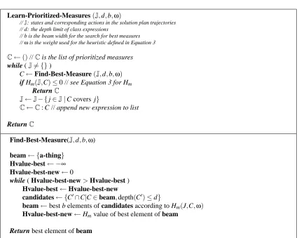
Learn-Prioritized-Measures(J,d,b,ω)
//J: states and corresponding actions in the solution plan trajectories // d: the depth limit of class expressions
// b is the beam width for the search for best measures //ωis the weight used for the heuristic defined in Equation 3
C←()//Cis the list of prioritized measures while (J6={})
C←Find-Best-Measure(J,d,b,ω) if Hm(J,C)≤0 // see Equation 3 for Hm
ReturnC
J←J− {j∈J|C covers j}
C←C: C // append new expression to list
ReturnC
Find-Best-Measure(J,d,b,ω)
beam← {a-thing} Hvalue-best← −∞ Hvalue-best-new←0
while ( Hvalue-best-new>Hvalue-best ) Hvalue-best←Hvalue-best-new
candidates← {C0∩C|C∈beam,depth(C0)≤d}
beam←best b elements of candidates according to Hm(J,C,ω)
Hvalue-best-new←Hmvalue of best element of beam
Return best element of beam
Figure 5: Pseudo-code for learning measures of progress
our heuristic learning has nothing to learn since its training signal is the difference between the observed distance in the training set and FF’s heuristic. Thus, we did not include such domains.
For each domain, we used 15 problems as training data, with the solutions being generated by FF. We then learned all three types of control knowledge (heuristics, taxonomic decision lists, and measures of progress) in each domain and used that knowledge to solve the remaining problems, which were typically more challenging than the training problems. We used each form of control knowledge as described in Section 4. For the case of the policy representations (taxonomic decision lists and measures of progress), we used FF’s RPL heuristic as the heuristic function and used a fixed policy-execution horizon of 50.