Unit 1
Lesson 7: Simplex Method Ctnd.
Learning outcomes:
• Set up and solve LP problems with simplex tableau.
• Interpret the meaning of every number in a simplex tableau.
Dear students, today we discuss small cases or case-lets on the above topic. The situations presented below are real business problems, modified slightly to suit our purpose.
We start now.
Case-let-1
A firm makes air coolers of three types and markets these under the brand name “Symphony”.
The relevant details are as follows:-
Profit / unit (Rs.)
300 Product A (hrs. / unit)
700 Product B (hrs. / unit)
900 Product C (hrs,/ unit)
Totoal hrs. available
Designing 0 10 20 320
Manufacturing 60 90 120 1600
Painting 30 40 60 1120
What Qty. of each product must be made to maximize the total profit of the firm?
Solution
30 X1 +40 X2 + 60 X3 ≤1120 Introducing slacks:
Maximize: 300 X1 +700 X2 + 900 X3 +0S1+ 0S2+ 0S3 Subject to: 0 X1 +10 X2 + 20 X3 +S1+ 0S2+ 0S3 =320 60 X1 +90 X2 + 120 X3 +0S1+ S2+ 0S3 =1600 30 X1 +40 X2 + 60 X3 +0S1+ 0S2+ S3 =1120 1st Tableau
CJ(Rs.) 300 700 900 0 0 0
(Rs.) Basic Act.
Qty. X1 X2 X3 S1 S2 S3
0 S1 320 0 10 20 1 0 0
0 S2 1600 60 90 120 0 1 0
0 S3 1120 30 40 60 0 0 1
ZJ 0 0 0 0 0 0 0
CJ - ZJ 300 700 900 0 0 0
Pivot column = X3 Pivot –row = S2
= = = 3 56 60 1120 : , 3 40 120 1600 : , 16 20 320 :
S1 S2 S3
Pivot element = 120
Pivot row updating : ,0
120 1 , 0 , 1 , 4 3 120 90 , 2 1 120 60 , 3 40 120 1600 = = =
Up-dating S1row: Updating S3 row:
3 160 3
40 20
320 =
− x 320
3 40 60 20 1 = − x 10 2 1 120
0 =−
− X 0
2 1 60
30 =−
− X 5 4 3 20
20 =−
− x 5
4 3 60
40 =−
− X
(
20 0)
51− x = 0−
(
60x0)
=06 1 120
1 20
0 = −
− x 2 1 120 1 60
0 = −
− x
(
20 0)
0IInd Tableau
Cj (Rs.)
(Rs.) Basic Act. Qty. 300 x1 700 x2 900 X3 S1 0 S2 0 S3 0 0 900 0 S1 X3 S3 Zj (Rs.) Cj-Zj (Rs.) 160/3 40/3 320 2000 -10 ½ 0 450 -150 -5 ¾ -5 675 25 0 1 0 900 0 1 0 0 0 0 -1/6 1/120 -1/2 15/2 -15/2 0 0 1 0 0
Since, There is still one + ve term in row, pivoting is requd. Pivot – Column = x2
Pivot – row =
=− ÷ = ( .) 5 320 : , 9 160 4 3 3 40 : ), 3 ( 5 3 160
: 3 3
1
3 S Notconsidere d x S Notconsi
x
Pivot – element =3/4 Pivot-row updating:
0 , 90 1 4 3 120 1 , 0 , 3 4 4 3 1 , 1 , 3 2 4 3 2 1 , 9 160 4 3 3
40÷ = ÷ = ÷ = ÷ =
Updating S1 row: Updating S3 row:
9 1280 9 160 5 3 160 = − − x 9 3680 9 160 5
320 =
− − x 3 20 3 2 5
10 =
− − − x 3 10 3 2 5 =
− − x 0
(
5 1)
05− =
− x −5−
(
−5x1)
=03 20 3 4 5
0 =
− − x 3 20 3 4 5 =
− − x 0
(
5 0)
11− − x = 0−
(
−5x0)
=09 1 90 1 5 6 1 − = − − − x 9 4 90 1 5 6 1 − = − − x −
(
5 0)
0IIIrd Tableau
Cj (Rs.)
(Rs.) Basic Act. Qty. 300 x1 700 x2 900 x3 S1 0 S2 0 S3 0 0
700 0
x1 S2 S3 Zj (Rs.) Cj-Zj (Rs.)
1280/9 160/9 3680/9 112000
-20/30 2/3 10/3 1400/3 -500/3
0 1 0 700 0
20/3 4/3 20/3 2800/3 -100/3
1- 0 0 0 0
1/9 1-90 -4/9 70/9 -70/9
0 0 1 0 0
Since Cj – Zj row has no. + ve value left.
∴It is the optional soln.
Case-let-II
Two materials A & B are required to construct table & book cases. For one table, 12 units of A & 16 units of B are required while for a book case 16 units of A and 8 units of B are required. The profit on book case is Rs 25 and Rs 20 on a table. 100 units of A & 80 units of B are available. Formulate as a Linear programming problem & determine the optimal number of book cases & tables to be produced so as to maximise the profits.
Solution
Let x1 = no. of unit of tables to be produced, and
X2 = no. of unit of book cases to be produced. Formulating as a LP problem, we have:-
Maximise Z =20x1 +25x2 ( objective function ) Subject to the constraints: 12x1+16x2 ≤100
16 80
0
00 80 8 2
1+ x ≤
x
, 2 1 x ≥
x
Introducing the slack variable, we have:
Re-writing as: = + + + 80 100 100 1 0 1 8 16 16 12 2 1 2
1 x S S
x
or P1x1+P2x2 +P3S1+P4S2 =Po ∴ our problem becomes Maximise
Subject to F =20x1+25x2 +0×S1+0×S2 …(1) Where P1x1+P2x2 +P3S1+P4S2 = Po …(ii)
= = + + 8 16 16 13 0 1 0 1 80 100 2 2 4 2
0 P P P P
P
element of Cj row are values of Po, P2,P4,P1, in (i) by comparing with (2) i.e. elements of Cj are 0, 0, 20, 25.
Simplex Method
Cj 0 0 0 20 25 Ratio
Vectors Po P2 P4 P1 P3
0 P3 100 1 0 12 16 100/16=6.25
0 P4 80 0 1 16 0 80/8=10
Zj 0 0 0 0 0 6.25 is least ratio
Zj – Cj
0 0 0 20 25 ∴ replaced vector is P2
R1 is
16 1
R
R2 = R2 – R1 x 8/16
Since 25 is the most postive No. in row C4 - Z4 ∴
Replacing vector is P2 25 P2
4
25 1/16 0
4 3 1 4 25 / 4 5 = 3 25 =8.33
0 P4 30
3 1
− 1 10 0 30/10=3
Zj 4 625 16 25 0 4 75 25 R1 R2 Stage I R1 R2 Stage I Zj –
Cj 6254 1625 0 −45 0
Θ 3 is least ratio
∴ replaced vector is P4
Θ 4 5
− is least – ve no.
∴ replaced vector is P1
10 1 2 R is R
R1 = R – R2
40 3 10 4 / 3 2 1 R R − =
R1 25 P2 4 1/10 /3/40 0 1
R2 20 P4 3 -1/20 1 1 0
Stage I Zj 160 1.5 1/8 20 25
Zj – Cj 160 1.5 1/8 0 0
Since in stage III all elements of row Zj – Cj are +ve or zero, hence an optimal solution has been achieved.
The solution is given by column is Stage III. 2
1 0 3P 4P
P = +
∴
compare it with P1x1+P2x2+P3S1+P4S2 = P0 0 ,
0 , 4 ,
3 2 1 2
1 = x = S = S = x
Note I. the elements of row Zj is the sum of product of corresponding elements of column Cj with Po,P3,P4,P1,P2 respectively.
For example in stage II, the elements of row Zj are
4 625 30 0 4
25+ =
x x
25
16 25 2
1 0
16 1
− =
+ x
x
25
25x 0+0 x 1=0
4 75 10 0 4
3+ =
x x
25
25 x 1 + 0x 0 =25.
Note 2. When we replace vector P2 in place of P3 in stage II, the elements to left of P3 under column Cj is also changed.
Note. To check the results. At x=3, x2 = 4
Constraints are 12x1+16x2 =36+64=100≤100 16x1+8x2 =48+32=80≤80
Case-let-III
Solution
Let no. of bicycles and scooters produced by x and y units respectively.
∴ L.P. problem is Maximize P = 45x + 55y Subject to 6x+3y≤120
4x+10y ≤180,x≥0,y ≥0
Introducing the slack variables, we get 120
3
6x+ y2 +S1+ 180 10
4x+ y2+S2+
writing it in vector form
…(1) = + + + 180 120 1 0 0 1 4 3 4 6 2 1 S S y x or P1x+P2y+p2S1+P4S2=P0
Θ Our L.P.P is Max, P=45x+55y+OS1+OS2
ΘSubject to P1x + P2y+P3S1 + P4S2=Po …(2) Comparing (1) and (3), we have
= = = 1 0 , 0 1 , 10 3 ' 4 6 4 3 2
1 P P P
P ' 180 120 = o P
The elements of row are value of
Po, P2,P4,P1,P3, in (1) by comparing it with (2) i.e., element of row are o, o, 45,45.,55.
Note. The element of row are sum of product of corresponding element of columns and column vectors
Simplex Method
Cj 0 0 0 45 55
Vectors Po P3 P4 P1 P2
0 P3 120 1 0 6 3
0 P4 180 0 1 4 10
Zj 0 0 0 0 0
R1
R2
Stage I
Zj-Cj 0 0 0 -45 -55
Ratio 45 4 / 180 41 /
40 α = =
α
∴ 20 is least ratio, so replace vector is P3
Θ- 55 is least no. in row Zj-Cj, ∴replacing vector
is P1
Row
6 4 1 2 31 41 1 2
2 − × R −R × a
a R
=R
R .
Further calculations are left to the students as an exercise.
Case-let-IV
.A firm has the following availabilities :
Type-available Amount-available (kg)
Wood Plastic Steel
240 370 180
The firm produces two products A & B having a selling price of Rs. 4 per unit & Rs. 6 per unit respectively. The requirements for the manufacture of A & B are as follows:
Requirements of (kg) Product
Wood Plastic Steel A
B
1 3
3 4
2 1
Formulate as a LP problem & solve by using the simplex method to maximise the gross income of the firm.
Case-let-V
Ace- advantage Ltd. faces the following situation: Media available - electronic (A) & print (B) Cost of available in - media A: Rs.1000
Media B: Rs.1500
Annual advertising budget - Rs. 20000 The following constraints are applicable:
Electronic Media (A) can not have more than 12 advertisements in a year and not less than 5 advertisement must be placed in the print media (B). The estimated audience are as follows:
Electronic media (A) - 40000 Print media (B) - 55000
Case-let-VI
Khalifa & sons sells two different books B1 & B2 at a profit
margin of Rs. 7 and Rs. 5 per book respectively. B1 requires 5
units of raw material & B2 requires 1 units of raw material. The
maximum availability of raw materials is limited to 15units. To
maintain the high quality of books, it is desired to follow the given
quality constraint: 3x1 + 7x2
≥
21. Formulating
As a LP model determine the optimal solution.
Dear students, we have now reached the end of our discussion scheduled for today. See you all in the next lecture.
Unit 1
Lesson 9 :
The Big M MethodLearning outcomes
• The Big M Method to solve a linear programming problem.
In the previous discussions of the Simplex algorithm I have seen that the method must start with a basic feasible solution. In my examples so far, I have looked at problems that, when put into standard LP form, conveniently have an all slack
starting solution. An all slack solution is only a possibility when all of the
constraints in the problem have <= inequalities. Today, we are going to look at methods for dealing with LPs having other constraint types.
Remember that simplex needs a place to start – it must start from a basic feasible solution then move to another basic feasible solution to improve the objective value.
With these assumptions, I can obtain an initial basic feasible solution /dictionary by letting all slack variables be basic, all original variables be non basic
Obviously, these assumptions do not hold for every LP. What do I do when they don’t?
When a basic feasible solution is not readily apparent, the Big M method or the two-phase simplex method may be used to solve the problem.
The Big M Method
If an LP has any > or = constraints, a starting basic feasible solution may not be readily apparent.
The Big M method is a version of the Simplex Algorithm that first finds a basic feasible solution by adding "artificial" variables to the problem. The objective function of the original LP must, of course, be modified to ensure that the artificial variables are all equal to 0 at the conclusion of the simplex algorithm.
Steps
1. Modify the constraints so that the RHS of each constraint is nonnegative (This requires that each constraint with a negative RHS be multiplied by -1. Remember that if you multiply an inequality by any negative number, the direction of the inequality is reversed!). After modification, identify each constraint as a <, >, or = constraint. 2. Convert each inequality
slack variable si; and if constraint i is a > constraint, we subtract an
excess variable ei).
3. Add an artificial variable ai to the constraints identified as > or = constraints at the end of Step 1. Also add the sign restriction ai > 0.
4. If the LP is a max problem, add (for each artificial variable) -Mai to the objective function where M denote a very large positive number.
5. If the LP is a min problem, add (for each artificial variable) Mai to the objective function.
6. Solve the transformed problem by the simplex . Since each artificial variable will be in the starting basis, all artificial variables must be
eliminated from row 0 before beginning the simplex. Now (In choosing the entering variable, remember that M is a very large positive number!).
If all artificial variables are equal to zero in the optimal solution, we have found the optimal solution to the original problem.
If any artificial variables are positive in the optimal solution, the original problem is infeasible!!!
Let’s look at an example.
Example 1
Minimize z = 4x1 + x2 Subject to:
3x1 + x2 = 3 4x1 + 3x2 >= 6 x1 + 2x2 <= 4
x1, x2 >= 0
By introducing a surplus in the second constraint and a slack in the third
we get the following LP in standard form:
Minimize z = 4x1 + x2 Subject to:
3x1 + x2 = 3 4x1 + 3x2 – S2 = 6 x1 + 2x2 + s3 = 4
x1, x2, S2, s3 >= 0
must use artificial variables. If we introduce the artificial variables R1 and R2
into the first two constraints, respectively, and MR1 + MR2 into the objective
function, we obtain:
Minimize z = 4x1 + x2 + MR1 + MR2 Subject to:
3x1 + x2 + R1 = 3 4x1 + 3x2 – S2 + R2 = 6 x1 + 2x2 + s3 = 4
x1, x2, S2, s3, R1, R2 >= 0
We can now set x1, x2 and S2 to zero and use R1, R2 and s3 as the starting basic feasible solution.
In tableau form we have:
Basic z x1 x2 S2 R1 R2 s3 Solution
z 1 -4 -1 0 -M -M 0 0
R1 0 3 1 0 1 0 0 3
R2 0 4 3 -1 0 1 0 6
s3 0 1 2 0 0 0 1 4
At this point, we have our starting solution in place but we must adjust our z-row to reflect the fact that we have introduced the variables R1 and R2 with non-zero coefficients (M).
We can see that if we substitute 3 and 6 into the objective function for R1 and R2, respectively, that z = 3M + 6M = 9M. In our tableau, however, z is shown to be equal to 0. We can eliminate this inconsistency by
substituting out R1 and R2 in the z-row. Because each artificial variable’s
column contains exactly one 1, we can accomplish this by multiplying each of the first two constraint rows by M and adding them both to the current z-row.
New z-row = Old z-row + M*R1-row + M*R2-row
Old z-row: (1 -4 -1 0 -M -M 0 0 ) + M*R1-row: (0 3M M 0 M 0 0 3M )
+ M*R2-row: (0 4M 3M –M 0 M 0 6M )
Our tableau now becomes
Basic z x1 x2 S2 R1 R2 s3 Solution
z 1 -4+7M -1+4M -M 0 0 0 9M
R1 0 3 1 0 1 0 0 3
R2 0 4 3 -1 0 1 0 6
s3 0 1 2 0 0 0 1 4
Now we have the expected form for our starting solution.
We now apply the simplex method as before. Since this is a minimization problem we select the entering variable with the most positive objective row coefficient. In this case, that is x1. Calculating the intercept ratios we get:
R1 – 3/3 = 1 R2 – 6/4 = 1.5 s3 -- 4/1 =
So we select R1 as our leaving variable.
Performing the Gauss-Jordan row operations, we obtain the new tableau:
Basic z x1 x2 S2 R1 R2 s3 Solution
z 1 0 (1+5M)/3 -M (4-7M)/3 0 0 4+2M x1 0 1 1/3 0 1/3 0 0 1
R2 0 0 5/3 -1 -4/3 1 0 2
s3 0 0 5/3 0 -1/3 0 1 3
In this tableau, we can see that x2 will be our next entering variable and R2 will leave.
We can thus see that the simplex algorithm will quickly remove both R1 and R2 from the solution just as we intended when we assigned them the
coefficient of M in the objective function. If we continue to apply the simplex algorithm, we will find that the optimal solution is:
x1 = 2/5 x2 = 9/5 S2 = 1
with z = 17/5
The use of the penalty M may not always force the artificial variable to zero level by the final iteration. This can occur in the case where the given LP has no feasible solution. If any artificial variable is positive in the final iteration than the LP has no feasible solution space.
Theoretically, the application of the M technique requires that M approaches infinity but to computerize the solution algorithm, M must be finite while being “sufficiently large.” The pitfall in this case is, however, if M is too large it can lead to substantial round-off error yielding an incorrect optimal solution. For this reason, most commercial LP solvers do not apply the M-method but use, rather, an artificial variable method called the two-phase method. For educational purposes, TORA, allows the implementation of the M-method with a user selected value for M where M is sufficiently large to allow solution of the problem. The definition of the term “sufficiently large” is dependent upon the problem in question and requires some judgment for implementation.
Example 2 Minimise z = 2x1 -3x2 + x3
subject to
3x1 -2x2 + x3 ≤ 5, x1 +3x2 -4x3 ≤ 9, x2 +5x3 ≥ 1,
x1 + x2 + x3 = 6, x1, x2, x3 ≥ 0.
Solution We obtain the linear programming problem: minimise x8 subject to
3x1 -2x2 + x3 + x4=5,
x1 +3x2 -4x3 + x5=9,
x1 + x2 + x3 + x6=6,
- x2 -5x3 + x7=-1,
-2x1 +3x2 - x3 + x8=0,
x1,..., x7 ≥ 0,
•
where x6 is an artificial variable. In tableau T1 of Table 1, pivoting about y33
(= 1) removes a6 from the basis. The rows of tableau T2 are then
rearranged to give tableau T3 so that the bad row is below the others, and
column a6 is ignored from here on. Pivoting in T3 about y12 (= 7) gives
tableau T4 which has the basic feasible solution (0, 33/7, 9/7, 92/7, 0, 0,
71/7, - 90/7). This has x6 = 0 and is an optimal solution, so x1 = 0, x2 =
33/7, x3 = 9/7 is an optimal solution of the original problem with optimal
Min z = 2x1+3x2
s.t.
1/2x1+1/4x2≤ 4………1
x1+3x2≥ 20………2
x1+x2=10………3
x1,x2 ≥ 0
Step1: Make the right hand side of all constraints positive.
We don’t have any negative right hand side.
Step2:Identify each constraint which is ≥ or=.
Constraints 2 and 3 apply the above conditions.
Step3: For each<= constraint add a slack variable and for each constraint subtract an excess variable to make them equalities.
1……….1/2x1+1/4x2+s1 =4
2………..x1+ 3x2 -e1=20
Step4:For each>=or = constraint add an artificial variable ai(ai’s>0),which is to be chosen in the starting bfs.
2……….x1+3x2-e1+a2=20
3……….x1+x2+ +a3=10
Step5: If the LP is a min add +Mai to the objective function. If it is
a max add –Mai to the objective function. Here M represents a very big number such that in the min problem +Mai is arbitrarily large so that ai the artificial variable is best to be chosen as zero, which we
require . Similar reasoning applies in the max problem.
Min z =2x1+3x2+Ma2+Ma3
are zero we find the solution, but if they are not equal to zero then we don’t have a optimal solution. Thus, original LP is infeasible.
After these steps we have the LP:
Min z=2x1+3x2+Ma2+Ma3
st
1/2x1+1/4x2+s1 =4
x1+3x2 -e1+a2=20
x1+x2 +a3=10
After all, we have the table:
In the optimal solution, we have: {z,s1, x2, x1}={25,1/4,5,5}. Since
we don’t have any of artificial variables a1and a2in the optimal
solution, the solution is feasible. If any of the artificial variablesa1,
a2were not equal to zero then we would have infeasibility as
described below:
Min z=x1+3x2
1/2x1+1/4x2 ≤ 4
x1+3x2 ≥ 10
x1+x2 =10
After going through all the steps described above we end with the optimal tableau:
In the above example, we have the optimal tableau since reduced costs of all non basic variables are non positive. However note that the optimal solution contains the very big number M, which should not have been the case for a min problem, thus we say that our original LP was infeasible. We also say that from the fact that we have the artificial variablea2 in the basic variables, which shouldn’t have been the case for a feasible LP.
Example 3
Maximize Z = x1 + 5x2
Subject to: 3x1 + 4x2 £ 6
x1 + 3x2 ³ 2
Where x1, x2 ³ 0
Solution
Introducing slack and surplus variables
3x1 + 4x2 + x3 = 6
x1 + 3x2 – x4 = 2
Where:
x3 is a slack variable
x4 is a surplus variable.
Now if we let x1 and x2 equal to zero in the initial solution, we will have x3 = 6 and
x4 = –2, which is not possible because a surplus variable cannot be negative.
Therefore, we need artificial variables.
Maximize x1 + 5x2 – MA1
Subject to:
3x1 + 4x2 + x3 = 6
x1 + 3x2 – x4 + A1 = 2
Where:
x1 ³ 0, x2 ³ 0, x3 ³ 0, x4 ³ 0, A1 ³ 0
Cj 1 5 0 0 –M
CB Basic
variables B
x1 x2 x3 x4 A1 Solution
values b (= XB)
0 x3 3 4 1 0 0 6
–M A1 1 3 0 –1 1 2
Zj – Cj –M –
1
–3M – 5
0 M 0
Here, a11 = 3, a12 = 4, a13 = 1, a14 = 0, a15 = 0, b1 = 6
a21 = 1, a22 = –3, a23 = 0, a24 = –1, a25 = 1, b2 = 2
Calculating Zj – Cj
First column = 0 * 3 + (–M) * 1 – 1 = –M – 1 Second column = 0 * 4 + (–M) * 3 – 5 = –3M–5 Third column = 0 * 1 + (–M) * 0 – 0 = 0
Fourth column = 0 * 0 + (–M) * (–1) – 0 = M Fifth column = 0 * 0 + (–M) * 1 – (–M) = 0
Choose the smallest negative value from Zj – Cj. Substitute M = 0
Minimum (6 / 4, 2 / 3) = 2 / 3
So second row is the element row. Here, the pivot (key) element = 3. Therefore, A1 departs and x2 enters.
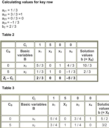
Calculating values for table 2
Calculating values for first row
a11 = 3 – 1 * 4 / 3 = 5 /3
a12 = 4 – 3 * 4 / 3 = 0
a13 = 1 – 0 * 4 / 3 = 1
a14 = 0 – (–1) * 4 / 3 = 4 / 3
b1 = 6 – 2 * 4 / 3 = 10 / 3
Calculating values for key row
a21 = 1 / 3
a22 = 3 / 3 =1
a23 = 0 / 3 = 0
a24 = –1 / 3
b2 = 2 / 3
Table 2
Cj 1 5 0 0
CB Basic
variables B
x1 x2 x3 x4 Solution
values b (= XB)
0 x3 5 / 3 0 1 4 / 3 10 / 3
5 x2 1 / 3 1 0 –1 / 3 2 / 3
Zj – Cj 2 / 3 0 0 –5 / 3
Table 3
Cj 1 5 0 0
CB Basic variables
B
x1 X2 x3 x4 Solution
values b (= XB)
0 x4 5 / 4 0 3 / 4 1 5 / 2
Zj – Cj 11 / 4 0 5 / 4 0
Since all the values of Zj – Cj are positive, this is the optimal solution.
x1 = 0, x2 = 3 / 2
Unit 1
Lesson 11: Duality in linear programming
Learning objectives:
• Introduction to dual programming.
• Formulation of Dual Problem.
Introduction
For every LP formulation there exists another unique linear programming
formulation called the 'Dual' (the original formulation is called the 'Primal'). The - Dual formulation can be derived from the same data from which the primal was formulated. The Dual formulated can be solved in the same manner in which the Primal is solved since the Dual is also a LP formulation.
The Dual can be considered as the 'inverse' of the Primal in every respect. The column coefficients in the Primal constrains become the row co-efficients in the Dual constraints. The coefficients in the Primal objective function become the right hand side constraints in the Dual constraints. The column of constants on the right hand side of the Primal constraints becomes the row of coefficients of the dual objective function. The 'direction of the inequalities are reversed. If the primal objective function is a 'Maximization' function then the dual objective function is a 'Minimization' function and vice-versa.
The concept of duality is very much in useful to obtain additional information about the variation in the optimal solution when certain changes are effected in the constraint efficient, resourse availabilities and objective function co-efficients. This is termed as post optimality or sensitivity analysis.
Dual Problem Construction:
- If the primal is a maximization problem, then its dual is a minimization problem (and vise versa).
- Use the variable type of one problem to find the constraint type of the other problem.
- Use the constraint type of one problem to find the variable type of the other problem.
- The matrix coefficients of the constraints of one problem is the transpose of the matrix coefficients of the constraints for the other problem. That is, rows of the matrix becomes columns and vise versa.
Dual
Formation
Following are the steps adopted to convert primal problem into its dual.
Step 1. For each constraint in primal problem there is an associated variable in dual problem.
Step 2. The elements of right hand side of the constraints will be taken as the co-efficient of the objective function in the dual problem.
Step 3. If the primal problem is maximization, then its dual problem will be minimization and vice versa.
Step 4. The inequalities of constraints should be interchanged from >= to <= and vice versa and the variables in both the problems and non-negative.
Step 5. The row of primal problem are changed to columns in the dual problem. In other words the matrix A of the primal problem will be changed ti its transpose (A) for the dual problem.
Step 6. The co-efficient of the objective function will be taken the right hand side of the constraints of the dual problem.
Problems and Solutions
An example will clarify the concept basis. Consider the following 'Primal' LP formulation
Example 3.1,
MaXimize 12x1 + 10x 2
subject to 2X1 + 3X2 <= 18 2X1 + X2 <= 14 X1, X21 >= 0 Solution 3.1,
The 'Dual' formulation for this problem would be Minimize 18Y1 + 14Y2
subject to 2Y1 + 2Y2 >= 12 3Y1 + Y2 >= 10 Y1 >= 0, Y2 >= 0 Note the following:
2. The co-efficient of the Primal objective function namely, 12 and 10 have become the constants in the right hand side of the Dual constraints. 3. The constants of the Primal constraints, namely 18 and 14, have become
the co-efficeint in the Dual obejctive function.
4. The direction of the inequalities have been reserved. The Primal
constraints have the in equalities of::; while the Dual constraints have the inequalities of ~ .
5. While the Primal is a 'Maximization' problem the Dual is a 'Minimization' problem
Why construct the Dual formulation? This is for a number of reasons. The solution to the dual problem provides all essential information about the solution to the Primal problem. For an LP problem, the solution can be determined either by solving the original problem or the dual problem. Sometimes it may be easier to solve the Dual problem rather than the Primal problem. (For instance, when the primal involves few variables but many constraints.)
Example 3.2,
Obtain the dual problem of the following primal formulation. Maximize Z = 2X1 + 5X2 + 6X3
Subject to 5X1 + 6X2 -X3 <= 3 -2x1 + X2 + 4X3 <= 4 X1 - 5X2 + 3X3 <= 1 -3X1 - 3X2 + 7X3 <= 6 X1, X2, X3 >= 0
Solution 3.2,
Step 1 : Write the objective function of the Dual. As there are four constraints in the primal, the objective function of the dual will have 4 variables.
Minimize r* = 3W1 + 4W2 + W3 + 6W4
Step 2 : Write the constraints of the dual. As all the constraints in the primal are '<', the constraints in the dual will be '>'. The column COM+ efficients of the primal become the row co-efficients of the dual.
Constriants. 5W1 - 2W2 + W3 - 3W4 >= 2 6W1 + W2 - 5W3 -W4 >= 5 -W1 + 4W2 + 3W3 + 7W4 >= 6
Subject to : 5W1 - 2W2 + W3 - 3W4 >= 2 6W1+ W2 - 5W3 - 3W4 >= 5 - W1 + 4W2 + 3W3 + 7W4 >= 6 W1, W2, W3, W4 >= 0
Example 3.3,
Obtain the dual of the- following linear programming problem.
Minimize Z = 5X1 -6X2 + 4X3 Subject to the
constriants :
3X1 + 4X2 + 6X3 >= 9 X1 + 3X2 + 2X3 >= 5 7X1 - 2X2 - X3 >= 10 X1 - 2X2 + 4X3 >= 4 2X1 + 5X2 - 3X3 >= 3 X1, X2, X3 >= 0
Solution 3.3,
In this problem one of the primal constraints (namely 7X1 - 2X2 - X3 <=10) is a "<= ", constraints while all the other are ">=”I constraints. The dual cannot be worked out unless all the constraints are in the same direction. To convert this into ">=” constraint, multiply both the sides of the equation by "-" sign. After multiplying the constraint by "-". sign, it will become 7x1 + 2x2 + x3 >= -10. Now all the constraints are in the same direction and the dual can be worked out.
The dual formulation is :
Maximize Z = 9W1 + 5W2 - 10W3 + 4W4 + 3W5 Subject to :
3W1 + W2 - 7W3 + W4 + 2W5 <= 5 4W1 + 3W2 + 2W3 - 2W4 + 5W5 <= -6 6W1 + 2W2 + W3 + 4W4 + -3W5 <= 4
Linear Programming
Background
Linear programming deals with problems such as maximising profits, minimising costs or ensuring you make the best use of available resources. From an applications perspective, mathematical (and therefore, linear) programming is an optimisation tool, which allows the rationalisation of many managerial and/or technological decisions. An important factor for the applicability of the mathematical programming methodology in various contexts, is the computational difficulty of the analytical models. With the advent of modern computing technology, effective and efficient algorithmic procedures can provide a systematic and fast solution to these models.
The seeds of linear programming were sown during World War II when the military supplies and personnel had to be moved efficiently. Although linear programming problems can be very complicated, which is to be expected since they are real-world problems, the principles can be understood by starting with simple problems that can be solved with GCSE algebra. Two-dimensional Linear programming can be solved graphically. Problems with more than two variables (as is the case for most real world problems) can be solved by using a technique called the simplex method (Wood and Dantzig 1949, Dantzig 1949). The
Simplex algorithm was one of the first Mathematical Programming algorithms to be developed and it provides a powerful
computational tool, able to provide fast solutions to very large-scale applications, sometimes including hundreds of thousands of variables (i.e. decision factors). Its subsequent successful implementation in a series of applications significantly contributed to the acceptance of the broader field of Operational Research as a scientific approach to decision making. linear optimisation, is the problem of maximising a linear function over a convex polyhedron.
A Linear Programming problem is a special case of a Mathematical Programming problem. From an analytical perspective, a mathematical program tries to identify an extreme (i.e., minimum or maximum) point of a function, which furthermore satisfies a set of constraints. Linear programming is the specialisation of mathematical programming to the case where both, function f , called the
objective function, and the problem constraints are linear. Mathematical (and therefore, linear) programming is an optimisation tool,
which allows the rationalisation of many managerial and/or technological decisions required by contemporary applications. An important factor for the applicability of the mathematical programming methodology in various contexts, is the computational tractability of the resulting analytical models. The advent of modern computing technology means that effective and efficient algorithmic procedures exist to provide a systematic and fast solution to these models. For Linear Programming problems, the
Simplex algorithm provides a powerful computational tool, able to provide fast solutions to very large-scale applications, sometimes
including hundreds of thousands of variables. In fact, the Simplex algorithm was one of the first Mathematical Programming algorithms to be developed (Wood and Dantzig 1949, George Dantzig, 1947), and its subsequent successful implementation in a series of applications significantly contributed to the acceptance of the broader field of Operational Research as a scientific approach to decision making.
Linear programming is now used extensively in business, economics and engineering. An example of an engineering application would be maximising profit in a factory that manufactures a number of different products from the same raw material using the same resources. The constraints would be decided by the amounts of raw materials available. In the field of business and management, linear programming is a method for solving complex problems in the two main areas of product mix (where the technique may be used where it is difficult to decide just how much of each variable to use in order to satisfy certain criteria such as maximising profits or minimising costs, subject to certain constraints) and distribution of goods.
As with all types of mathematical modelling, the effective application of Linear Programming requires good understanding of the underlying modelling assumptions, and a pertinent interpretation of the analytical solutions obtained.
Graphical Method for solving problems with two variables
The graphical method for solving linear programming problems in two unknowns is as follows.
1. Define the variables 2. Define the constraints
3. Define the objective function (the function which is to be maximised or minimised) 4. Graph the feasible region.
5. Find the coordinates of the corner points.
Example:
A small factory produces two types of toys: trucks and bicycles. In the manufacturing process two machines are used: the lathe and the assembler. The table shows the length of time needed for each toy:
The lathe can be operated for 16 hours a day and there are two assemblers which can each be used for 12 hours a day. Each bicycle gives a profit of £16 and each truck gives a profit of £14. Formulate and solve a linear programming problem so that the factory maximises its profit.
Time on
lathe (hours) Time on assembler (hours)
Bicycle 2 2
Truck 1 3
Formulate the problem
Let x be number of bicycles made
Think about the simplifying assumptions that have been made. Times are given to the nearest hour. Costs, and hence profits, remain constant. There are enough skilled workers to work the machines for the number of hours they can be used.
Let y be number of trucks made.
Objective Function Maximise P = 16x + 14y
Subject to constraints Graphical solution
2x + y ≤ 16 Lathe 2x + 3y ≤ 24 Assembler x, y ≤ 0
Method 2: Profit Line
Draw a line through the origin parallel
to the gradient of the profit function. Move this line up the y-axis until it is just leaving the feasible region – the point at which it leaves the feasible region is the optimum value. Method 1: Tour of vertices
(0,8) profit = £112 (6,4) profit = £152 (8,0) profit = £128
Interpret the solution
Optimal solution is to make 6 bicycles and 4 trucks. Profit £152
Formulating a linear Programming in business and management
This is a simplified example will illustrates the way in which a problem relating to business is formulated. A large sub-contractor machines special parts to order. For one order he has two machines, X and Y
available. Unfortunately, the machines perform more effectively on some jobs than others. Machine Y can do 10 units per hour on contracts from Alpha Ltd., 12 per hour on components from Beater & Co. and 26 per hour on those from Chester Inc., while Machine X can produce 16, 9 and 10 units per hour respectively. However, this is complicated by certain constraints which are:
Maximum number of units per month of units from Alpha, Beater and Chester are 6,500, 4,440 and 800 per month respectively
the machines X and Y are restricted to working a maximum of 260 and 350 hours per month respectively. The problem is to find how many hours should each machine work to maximise profits. This is answered by plotting machine Y's hours against machine X's hours using mathematical models for the three suppliers and then solving these using linear programming.
1. Define the variables
Let the number of hours for machine X be x
Let the number of hours for machine Y be y
2. Define the constraints
The model for Alpha can be found by using the above data as follows:
Machine X can produce 16 units per hour so if it works x hours the total is 16x hours.
So the model for Alpha, which cannot exceed 6,500 is: 10y + 16x≤ 6500 and the model for Beater which cannot exceed 4,400 is: 12y + 9x≤ 4400.
and the model for Chester which cannot exceed 8,000 is: 26y + 10x≤ 8000.
3. Define the objective function
A profit model is necessary in order to find the conditions for maximum profit i.e. the optimum number of hours for X and for Y. In this case, the profits on each machine's output are: X = £40 per hour and Y = £24, so the total profit is P = 40x + 24y.
Because of the existence of only two variables (x and y) this can be solved by plotting the models on a graph
for the three suppliers and moving the profit model until it reaches the highest point of intersection of the
three supplier lines.
NOTE: With maximisation problems if the feasible region is not bounded, this method can be misleading: optimal solutions always exist when the feasible region is bounded, but may or may not exist when the feasible region is unbounded.
An example of a minimisation problem
Sometimes rather than maximising profits, you may be asked to minimise costs. In this case the feasible region could be unbounded, as can be seen in this example
Minimise C = 3x + 4y
subject to the constraints: 3x - 4y ≤ 12, x + 2y ≥ 4 x ≥1, y ≥ 0.
The feasible region for this set of constraints is shown on the graph. The following table shows the value of C at each corner point:
Point C = 3x + 4y
(1, 1.5) 3(1)+4(1.5) = 9 minimum
(4, 0) 3(4)+4(0) = 12 Therefore, the solution is x = 1, y = 1.5, giving the minimum value C = 9.
Simplex Method for Standard Maximisation Problem
To solve a standard maximisation problem using the simplex method, we take the following steps:
• Convert to a system of equations by introducing slack variables to turn the constraints into equations, and rewriting the objective function in standard form.
• Write down the initial tableau.
• Select the pivot column: Choose the negative number with the largest magnitude in the objective
row. Its column is the pivot column. (If there are two candidates, choose either one.) If all the numbers in the objective row are zero or positive then you have the optimal solution.
• Divide each R.H.S. value by the corresponding element in the pivot column - ignore negative ratios
and division by zero, this is called the ratio test. Of these test ratios, choose the smallest one. The corresponding number in the pivot column is the pivot.
• If necessary, divide the pivot row by the value of the pivot to make the pivot element one.
• Add/subtract multiples of the transformed pivot row to/from the other rows to create zeros in the pivot
column
• Go to Step 3.
Slack Variables
In order to enable problems to be converted into a format that can be dealt with by computer, slack variables are introduced to change the constraint inequalities into equalities. Each vertex of the feasible region would then be defined by the intersection of two lines where the variables equal zero.
The Simplex Method
variables, a graphical approach is no longer appropriate, so we use the simplex tableau, a tabular form of the algorithm which uses row reduction (remember Gaussian elimination?) to solve the problem.
Other types of problems: Simplex can be adapted to solve a range of problems, such as shortest path (minimisation), maximum flow (maximisation) and game theory (maximin).
Example: A small factory produces two types of toys: trucks and bicycles. In the manufacturing process two machines are used: the lathe and the assembler. The lathe can be operated for 16 hours a day and there are two assemblers which can each be used for 12 hours a day. Each bicycle gives profit of £16 and each truck gives a profit of £14. Formulate and solve a linear programming problem so that the factory maximises its profit.
The table shows the length of time needed for each toy: Lathe Assembler
Bicycle 2 hours 2 hours
Truck 1 hour 3 hours
P – 16x – 14y = 0 Introduce slack variables 2x + y + s1 = 16
2x + 3y + s2 = 24
Simplex tableau
Let x be number of bicycles made Formulate the
problem Let y be number of trucks made.
Maximise P = 16x + 14y Objective Function
Subject to constraints: Lathe
Assembler
Solve the problem
2x + y < 16 2x + 3y < 24
Graphical solution
By considering vertices
(8, 0) P = 16 X 8 = £128
(6, 4) P= (16 X 6) + (14 X 4) = £152 (0, 8) P = 14 X 8 =£112
Factory should make 6 bicycles and 4 trucks each day. Profit £152
Interpret solution
p x y s1 s2 ratio test
1 -16 -14 0 0 0
0 2 1 1 0 16 16/2=8
0 2 3 0 1 24 24/2=12
1 0 -6 8 0 128
0 1 0.5 0.5 0 8 8/0.5=16
0 0 2 -1 1 8 8/2=4
1 0 0 5 3 152
0 1 0 0.75 -0.25 6 0 0 1 -0.5 0.5 4
Reading from the tableau P = £152 x = 6 y = 4 s1 = 0 and s2 = 0
Factory should make 6 bicycles and 4 trucks each day. Profit £152
Three variable example
Number of bicycles Number of
trucks
Maximise P = 9x + 10y + 6z Subject to constraints
Initial Tableau
P x y z s1 s2 RHS Min ratio
1 -9 -10 -6 0 0 0
0 2 3 4 1 0 3 1
0 6 6 2 0 1 8
Pivot 1
P x y z s1 s2 RHS Min ratio
1 -2.333 0 7.3333 3.3333 0 10
0 0.6667 1 1.3333 0.3333 0 1
0 2 0 -6 -2 1 2 1
Pivot 2
P x y z s1 s2 RHS
1 0 0 0.3333 1 1.1667 12.333
0 0 1 3.3333 1 -0.333 0.3333
0 1 0 -3 -1 0.5 1
Solution:
P = 12⅓ when x = 1, y = ⅓, z = 0
≥ constraints
The simplex algorithm relies on (0,0) being a feasible solution. If it is not, then you add artificial variables a1, a2, etc. to all ≥ constraints which move us from (0,0) into the feasible region. You now need surplus (as opposed to slack) variables which are subtracted from the constraints as they tell us how much greater than the constraint line a point is. Then
introduce a new objective function Q = a1 + a2 + … which you must minimise, since when
Q = 0 you are in the feasible region and you can complete the simplex in the normal
A furniture manufacturer makes square dining tables, round dining tables and chairs. Each square table needs £40 of raw materials and takes 12 hours to make.Each round table needs £50 of raw materials and takes 14 hours to make. Each chair needs £40 of raw materials and takes 16 hours to make. He must make at least 4 times as many chairs as tables.
There are 500 hours available and £1500 of raw materials.Each chair makes £40 profit each square table makes £30 profit and each round table makes £35 profit
A company produces three soft toys, an antelope, a bear and a cat. For one day's production run it has available 11 m2 of fur fabric, 24 m2 of wool fabric and 30 glass eyes.
The antelope requires 0.5 m2 of fur fabric, 2 m2 of wool fabric and two eyes. Each sells at a profit of £3. The bear requires 1 m2 of fur fabric, 1.5 m2 of wool fabric and two eyes. Each sells at a profit of £5. The cat requires 1 m2 of fur fabric, 1 m2 of wool fabric and two eyes. Each sells at a profit of £2.
A small factory makes 2 types of inflatable boats, a 2 person and 4 person. Each 2 person boat requires 0.9 hours in the cutting department and 0.8 hours in the assembly department. Each four person boat requires 1.8 hours in the cutting
department and 0.5 hours in the assembly department. The company makes profit of £25 on each 2 person boat and £40 on each 4 person boat.The maximum hours available each month in the cutting department is 864 and the maximum hours available each month in the assembly department is 672.
A manufacturer makes three products X, Y and Z. They all require resources A, B, C and D which are in short supply. The table shows the amount of each resource needed and the profit on each product
A B C D
X 20 0 20 40
Y 50 20 40 30
Z 40 10 20 20
available 600 100 700 1800 profit
6 4 10
Jo is making raspberry and chocolate cakes for a charity fair
A raspberry cakes needs 200g of flour and 200g of sugar and 2 eggs
A chocolate cake needs 225g of flour and 150g of sugar and 2 eggs
There are 3Kg of flour, 2.5Kg of sugar and 28
eggs available.
A raspberry cake sells for £2.50 and a chocolate cake sells for £3.00
Brad makes and sells three types of birdfood A, B and C.
A contains 4 kg of bird seed, 2 suet blocks and 1 kg of nuts, B contains 5 kg of bird seed, 1 suet block and 2 kg of nuts and C contains 10 kg of bird seed, 4 suet blocks and 3 kg of nuts.
Each week Brad has 140 kg of bird seed, 60 suet blocks and 60 kg of nuts available for the packs. The profit made on each pack of A, B and C is £3.50, £3.50 and £6.50 respectively.
Anna is making birthday cards in 2 designs, flowers and boats, to sell.She has enough card to make 16 birthday cards but she needs to get them all made in the next 6 hours. Flower cards take 30 mins to make and sell for £1.25. Boat cards take 20 mins to make and sell for £1.40
maximise
P
=
35
x
+
30
y
+
40
z
subject to
4
x
+
10
y
+
4
z
≤
150
6
x
+
7
y
+
8
z
≤
250
x
+
y
−
4
z
≤
0
maximise
P
=
3
x
+
5
y
+
2
z
subject to
x
+
2
y
+
2
z
≤
22
4
x
+
3
y
+
2
z
≤
48
x
+
y
+
z
≤
15
maximise
P
=
25
x
+
40
y
subject to
3
x
+
6
y
≤
2880
8
x
+
5
y
≤
6720
maximise
P
=
6
x
+
4
y
+
10
z
subject to
2
x
+
5
y
+
4
z
≤
60
2
y
+
z
≤
100
2
x
+
4
y
+
2
z
≤
70
4
x
+
3
y
+
2
z
≤
180
maximise
P
=
2.5
x
+
3
y
subject to
8
x
+
9
y
≤
120
4
x
+
3
y
≤
50
3
x
+
2
y
≤
28
maximise
P
=
3.5
x
+
3.5
y
+
6.5
z
subject to
4
x
+
5
y
+
10
z
≤
140
2
x
+
y
+
4
z
≤
60
x
+
2
y
+
3
z
≤
60
maximise
P
=
1.25
x
+
1.4
y
subject to
x
+
y
≤
16
3
x
+
2
y
≤
36
maximise
P
=
25
x
+
25
y
subject to
2
x
−
y
≤
0
−
x
+
y
≤
0
P
x
y
z
s
t u rhs
1
−
35
−
30
−
40 0 0 0
0
0
4
10
4
1 0 0 150
0
6
7
8
0 1 0 250
0
1
1
−
4 0 0 1
0
P
x
y
z
s
t u rhs
1
−
3
−
5
−
2 0 0 0
0
0
1
2
2
1 0 0 22
0
4
3
2
0 1 0 48
0
1
1
1
0 0 1 15
P
x
y
s
t
rhs
1
−
25
−
40 0 0
0
0
3
6
1 0 2880
0
8
5
0 1 6720
P
x
y
z
s
t u v rhs
1
−
6
−
4
−
10 0 0 0 0
0
0
2
5
4
1 0 0 0
60
0
0
2
1
0 1 0 0 100
0
2
4
2
0 0 1 0
70
0
4
3
2
0 0 0 1 180
P
x
y
s
t u rhs
1
−
2.5
−
3 0 0 0
0
0
8
9
1 0 0 120
0
4
3
0 1 0 50
0
3
2
0 0 1 28
P
x
y
z
s
t u rhs
1
−
3.5
−
3.5
−
6.5 0 0 0
0
0
4
5
10
1 0 0 140
0
2
1
4
0 1 0 60
0
1
2
3
0 0 1 60
P
x
y
s
t rhs
1
−
1.25
−
1.4 0 0
0
0
1
1
1 0 16
0
3
2
0 1 36
P
x
y
s
t u rhs
1
−
25
−
25 0 0 0
0
0
2
−
1 1 0 0
0
0
−
1
1
0 1 0