U
NIVERSITY OF
T
RENTO
CIFREM
I
NTERDEPARTMENTAL
C
ENTRE FOR
R
ESEARCH
T
RAINING
IN
E
CONOMICS AND
M
ANAGEMENT
D
OCTORAL
S
CHOOL IN
E
CONOMICS AND
M
ANAGEMENT
MEASURING
P
RODUCTIVITY AND
T
ECHNOLOGICAL
P
ROGRESS
D
EVELOPMENT OF A CONSTRUCTIVE METHOD BASED ON
C
LASSICAL
E
CONOMICS AND
I
NPUT
-O
UTPUT TABLES
A DISSERTATION
SUBMITTED TO THE DOCTORAL SCHOOL OF ECONOMICS AND MANAGEMENT
IN PARTIAL FULFILLMENT OF THE REQUIREMENTS
FOR THE
D
OCTORAL DEGREE
(P
H
.D.)
IN
E
CONOMICS AND
M
ANAGEMENT
A
DVISORS
D
OCTORAL
C
OMMITTEE
Advisor:
Prof. Stefano Zambelli
Università degli Studi di Trento
Prof. Gabriella Berloffa
Università degli Studi di Trento
Co-Advisor:
Prof. Giuliana Passamani
Università degli Studi di Trento
Prof. Massimo Warglien
Università Ca’ Foscari di Venezia
Prof. Luca Zarri
Università degli Studi di Verona
R
EFEREE
C
OMMITTEE
Prof. Guglielmo Chiodi
Università di Roma la Sapienza
Prof. Giovanni Pegoretti
MEASURING
PRODUCTIVITY
AND
TECHNOLOGICAL PROGRESS
Development of a Constructive Method based on Classical Economics
and Input-output tables
A Dissertation submitted to the doctoral school of economics and
management in partial fulfillment of the requirements for the doctoral
degree (Ph.D) in Economics and Management, January 2010
by
Matteo Degasperi
Inter-Departmental Centre for Research Training in Economics and
Management of the Departments of Economics and of Information
Technologies and Business Studies (CIFREM)
University of Trento
Via Rosmini, 70
38122 Trento, Italy
Principal supervisor:
Prof. Stefano Zambelli
Professor of Economics
Department of Economics
University of Trento
Via Rosmini, 70
38122 Trento, Italy
Co-supervisor:
Prof. Giuliana Passamani
Professor of Economics
Department of Economics
Acknowledgements
Writing a doctoral thesis has been a complex and curious process and the
final result is a synthesis of the ideas of many minds. My simple role has
been to collect and reorganize the ideas of those who have preceded me in
this line of study, those who have worked with me, and those who while
not expert in this field have had the patience to listen and discuss with
me. Many people deserve gratitude for successful completion of my
dissertation.
My first thanks go to Professor Stefano Zambelli for having accepted to be
my supervisor and for giving me the passion and support to overcome this
challenge.
Another special thanks goes to Thomas Fredholm, with whom I have
worked very closely during the writing of my thesis.
I would also like to thank all the members of CIFREM and all the staff at
OPES for giving me the opportunity to work in an international and
professional environment.
I also wish to express my gratitude to Professor Charlotte Bruun and Prof.
Carsten Heyn-Johnsen for making my experience in Denmark a pleasant
one.
Finally, I would also like to thank my family for the support and
Contents
Acknowledgments
iii
List of Tables
viii
List of Figures
x
Introduction
xiii
I.1 Traditional approaches to measuring productivity xv
I.2 The model of Sraffa xxi
I.2.1 The standard system and the standard commodity xxvi
I.2.2 The subsystems xxviii
I.3 Structure of the thesis xxxi
I.4 Advantages of this approach to measuring productivity xxxii
I.4.1 The rejection of the aggregate production function xxxii
I.4.2 The use of production prices xxxiii
I.4.3 The scale invariance property of the wage-profit frontier xxxiii
I.5 Limitations of this approach to measuring productivity xxxiv
I.5.1 The use of input-output tables in value term xxxiv
I.5.2 Fixed capital xxxiv
I.5.3 The numéraire xxxv
I.6 Concluding remarks xxxv
References xxxvii
I Measures of productivity with a classical flavor: theory
and application
1
1 Productivity Accounting Based on Production Prices
3
1.1 Introduction 5
1.2 The Theoretical Model 5
1.3 Productivity Accounting 7
1.4 Algorithms and the Choice of Numéraire 8
1.5 Data 9
1.6 Analysing the Data 10
1.7 Conclusion 14
References 16
Appendices
19
1.A The Dataset 21
1.B A Note on the Numéraire 23
2 New Measures of sectoral Productivity
29
2.1 Introduction 31
2.2 Productivity measures based on classical tradition 32
2.3 The Theoretical models 33
2.3.1 Goodwin’s Normalized General Coordinates 33
2.3.2 Pasinetti’s vertical integration 34
2.3.3 Gossling’s subsystems 34
2.3.4 Sraffa’s reduction to dated quantities of labor and the reduction to
dated quantities of a commodity 37
2.4 New Indicators of sectoral productivity 38
2.4.1 Productivity indicator based on Goodwin’s Normalized General
coordinates 38
2.4.2 Productivity indicator based on Pasinetti’s vertical integration 39
2.4.3 Productivity indicators based on Gossling’s subsystems 39
2.4.4 Productivity indicators based on the reduction to dated quantities of a
commodity 41
2.5 Data 42
2.6 The Empirical investigation and comparison 42
2.7 Conclusions 47
References 49
3 Productivity in the Italian Regions: Development of
Alternative Indicators Based on Input-Output Tables
51
3.1 Introduction 53
3.2 Indicators 54
3.2.1 Indicators of Aggregate Productivity 54
3.2.2 Indicators of Sectoral Productivity 56
3.2.3 Indicators of Convergence 58
3.3 Source and Preparation of the Data and the Choice of Numéraire 59
3.4 Empirical Analysis 60
3.4.1 Aggregate Productivity and Technological Progress 60
3.4.2 Sectoral Productivity 63
3.4.3 Convergence 70
3.5 The behavior of Production Prices 75
3.6 Conclusions 77
References 79
Appendices
81
3.A Industry Classification and Aggregation 82
3.B Scale Invariance Property of the Wage-Profit frontier – A small
example 83
4. An Inquiry into the Choice of
Numéraire
89
4.1 Introduction 91
4.2 Theoretical Prologue 91
4.3 Criteria for the Choice of Numéraire: an example 92
4.4 The Procedure Adopted 93
4.4.1 The Sign Direction Approach 93
4.4.2 The Standard Deviation Approach 94
4.5 The empirical result 96
4.6 Toward a general case 98
4.7 Conclusions 100
References 101
5. An Inquiry into the Effect of Aggregation
103
5.1 Introduction 105
5.2 The Wage-Profit frontier 106
5.3 Data and the Choice of Numéraire 107
5.4 The Effect of Aggregation on the wage-profit frontier 107 5.5 A robustness check of the indicators of technological progress and
labor productivity 110
5.6 Conclusions 115
References 116
Appendices
117
5.A The Dataset 119
5.B Wage-profit Frontiers for Different Levels of Aggregation 120
5.C Correlation Coefficients 121
III Statistical Appendix
123
A.1. New Measures of sectoral Productivity
125
A.2. Productivity in the Italian Regions: Development of
List of Tables
I. Introduction
I.1 A production system with three commodities xxix
I.2Decomposition into subsystems of a production system with three
commodities xxx
I.3 Subsystem 1 xxx
2.New Measures of sectoral Productivity
2.1 Transactions in a three-sectors economy 35
2.2 Index based on the reduction to dated quantities of a commodity – US 2000 45 2.3 Index based on the reduction to dated quantities of a commodity – Germany
2000 46
2.4 Index based on the reduction to dated quantities of a commodity – France
2000 46
2.5 Index based on the reduction to dated quantities of a commodity – UK 2000 47
3.Productivity in the Italian Regions: Development of Alternative
Indicators Based on Input-Output Tables
3.1 Technological progress - values 61
3.2 Ranking of regions by technological progress 61
3.3 Labor productivity - values 62
3.4 Ranking of regions by labor productivity 62
3.5 Sectoral productivity index based on physical quantities – region’s relative
position in each sector in [2001] and {2004} 67
3.6 Sectoral productivity index based on production prices – region’s relative
position in each sector in [2001] and {2004} 68
3.7 Braviais-Pearson linear correlation coefficients between the two indexes of
sectoral productivity 69
3.8 Contemporary frontier - 2001 71
3.9 Contemporary frontier – 2004 72
3.10 Intertemporal frontier 73
4.An Inquiry into the Choice of
Numéraire
4.1 The sign direction approach 94
4.2 The standard deviation approach 95
4.3 The effect of numéraire on the likelihood of reverse capital deepening 99
5.An Inquiry into the Effect of Aggregation
5.1 Representation of the pattern of aggregation 108
5.2 Mean relative change of the area under the wage-profit frontiers 109
5.3 Technological progress- Relative position of each country in each time period
for different levels of aggregation of input-output tables 113
5.4 Labor productivity- Relative position of each country in each time period for
different levels of aggregation of input-output tables 114
5.6 Matrix of correlation coefficients – US 2000 121
5.7 Matrix of correlation coefficients – Germany 2000 121
5.8 Matrix of correlation coefficients – France 2000 121
5.9 Matrix of correlation coefficients – UK 2000 121
A.1.New Measures of sectoral Productivity
A.1.1 Productivity indicator based on Goodwin’s normalized general coordinates
for the US, Germany, France, the UK 126
A.2.Productivity in the Italian Regions: Development of
Alternative Indicators Based on Input-Output Tables
A.2.1 Index based on physical quantities – 2001 (values) 133
A.2.2 Index based on physical quantities – 2004 (values) 134
A.2.3 Index based on production prices– 2001 (values) 135
A.2.4 Index based on production prices – 2004 (values) 136
A.2.5 The Velupillai-Fredholm-Zambelli index 137
A.2.5 Classification of Production prices into four groups - 2001 165
List of Figures
I. Introduction
I.1 Wage-profit frontier in the particular case of standard system xxv
1.Productivity Accounting Based on Production Prices
1.1 The wage-profit frontiers for the US, Germany, France, and the UK 11
1.2 Technological progress 12
1.3 The NNP curves for the US, Germany, France, the UK 13
1.4 Labor productivity 14
1.5 Two different cases of technological progress 25
1.6 The arc of technology and the ray of technology 26
1.7 Technological progress 27
3.Productivity in the Italian Regions: Development of Alternative
Indicators Based on Input-Output Tables
3.1 Technological progress 61
3.2 Labor productivity 62
3.3 Index of sectoral productivity based on physical quantities 64
3.4 The Velupillai-Fredholm-Zambelli index 75
3.5 The NNP per unit of labor curves 84
3.6 The Wage-profit frontiers 84
4.An Inquiry into the Choice of
Numéraire
4.1 Results of the change of sign approach 96
4.2 Results of the standard deviation approach 97
5.An Inquiry into the Effect of Aggregation
5.1 Relative differences between the areas obtained by using 23-by-23 industries output tables and the areas obtained by using 19-by-19 industries
input-output tables 110
5.2 Wage-profit frontiers - 1970 120
5.3 Wage-profit frontiers - 2000 120
A.1.New Measures of sectoral Productivity
A.1.1 Productivity indicator based on Pasinetti’s vertical integration - US 127 A.1.2 Productivity indicator based on Pasinetti’s vertical integration - Germany 127 A.1.3 Productivity indicator based on Pasinetti’s vertical integration - France 128 A.1.4 Productivity indicator based on Pasinetti’s vertical integration - UK 128
A.1.5 Labor productivity indicator based on Gossling’s subsystems –US 129
A.1.6 Capital productivity indicator based on Gossling’s subsystems – US 129
A.1.7 Multi-factor productivity indicator based on Gossling’s subsystems – US 129
A.1.8 Labor productivity indicator based on Gossling’s subsystems – GER 130
A.1.9 Capital productivity indicator based on Gossling’s subsystems – GER 130
A.1.10 Multi-factor productivity indicator based on Gossling’s subsystems – GER 130
A.1.12 Capital productivity indicator based on Gossling’s subsystems- FRA 131 A.1.13 Multi-factor productivity indicator based on Gossling’s subsystems - FRA 131
A.1.14 Labor productivity indicator based on Gossling’s subsystems - UK 132
A.1.15 Capital productivity indicator based on Gossling’s subsystems- UK 132
A.1.16 Multi-factor productivity indicator based on Gossling’s subsystems - UK 132
A.2.Productivity in the Italian Regions: Development of
Alternative Indicators Based on Input-Output Tables
A.2.1 Production prices – Agriculture and Fishing 2001 138
A.2.2 Production prices – Agriculture and Fishing 2004 138
A.2.3 Production prices – Extraction of minerals 2001 139
A.2.4 Production prices – Extraction of minerals 2004 139
A.2.5 Production prices – Mfr.of Food, Beverages and Tobacco 2001 140
A.2.6 Production prices – Mfr.of Food, Beverages and Tobacco 2004 140
A.2.7 Production prices – Mfr.of Textiles, Wearing Apparel, Leather 2001 141 A.2.8 Production prices – Mfr.of Textiles, Wearing Apparel, Leather 2004 141
A.2.9 Production prices – Mfr.of Wood and Wood Products 2001 142
A.2.10 Production prices – Mfr.of Wood and Wood Products 2004 142
A.2.11 Production prices – Mfr.of Paper Products, Printing and Publishing 2001 143 A.2.12 Production prices – Mfr.of Paper Products, Printing and Publishing 2004 143
A.2.13 Production prices – Mfr.of Refined Petroleum 2001 144
A.2.14 Production prices – Mfr.of Refined Petroleum 2004 144
A.2.15 Production prices – Mfr.of Chemicals and Man-Made Fibers Etc.2001 145
A.2.16 Production prices – Mfr.of Chemicals and Man-Made Fibers Etc.2004 145
A.2.17 Production prices – Mfr.of Rubber Plastic Products 2001 146
A.2.18 Production prices – Mfr.of Rubber Plastic Products 2004 146
A.2.19 Production prices – Mfr.of Other Non Metallic Mineral Products 2001 147 A.2.20 Production prices – Mfr.of Other Non Metallic Mineral Products 2004 147
A.2.21 Production prices – Mfr. and Processing of Basic Metals 2001 148
A.2.22 Production prices – Mfr. and Processing of Basic Metals 2004 148
A.2.23 Production prices – Mfr.of Machinery and Equipment n.e.c. 2001 149
A.2.24 Production prices – Mfr.of Machinery and Equipment n.e.c. 2004 149
A.2.25 Production prices – Mfr.of Electrical and Optical Equipment 2001 150
A.2.26 Production prices – Mfr.of Electrical and Optical Equipment 2004 150
A.2.27 Production prices – Mfr.of Transport Equipment 2001 151
A.2.28 Production prices – Mfr.of Transport Equipment 2004 151
A.2.29 Production prices – Mfr.of Furniture, Mfr. n.e.c. 2001 152
A.2.30 Production prices – Mfr.of Furniture, Mfr. n.e.c. 2004 152
A.2.31 Production prices – Electricity, Gas and Water Supply 2001 153
A.2.32 Production prices – Electricity, Gas and Water Supply 2004 153
A.2.33 Production prices – Construction 2001 154
A.2.34 Production prices – Construction 2004 154
A.2.35 Production prices – Wholesale and Retail Trade 2001 155
A.2.36 Production prices – Wholesale and Retail Trade 2004 155
A.2.37 Production prices – Hotels and Restaurants 2001 156
A.2.38 Production prices – Hotels and Restaurants 2004 156
A.2.39 Production prices – Transport, Post and Telecommunications 2001 157
A.2.41 Production prices – Financial Intermediation, Insurance 2001 158
A.2.42 Production prices – Financial Intermediation, Insurance 2004 158
A.2.43 Production prices – Computer, Research and Development, Consultancy
2001 159
A.2.44 Production prices – Computer, Research and Development, Consultancy
2004 159
A.2.45 Production prices – Public Administration 2001 160
A.2.46 Production prices – Public Administration 2004 160
A.2.47 Production prices – Education 2001 161
A.2.48 Production prices – Education 2004 161
A.2.49 Production prices – Health Care Activities Etc. 2001 162
A.2.50 Production prices – Health Care Activities Etc. 2004 162
A.2.51 Production prices – Other Service Activities 2001 163
A.2.52 Production prices – Other Service Activities 2004 163
A.2.53 Production prices – Renting of Machinery and Equipment, Real Estate
Activities 2001 164
A.2.54 Production prices – Renting of Machinery and Equipment, Real Estate
The purpose of this introduction is to provide a background to facilitate the understanding of subsequent chapters. The first section describes the traditional approaches to measuring productivity, in order to identify the strengths and weakness of each of them. The second section illustrates the model of Sraffa in the case of single production and deepens some aspects related to the model that will be used in the dissertation. The third section describes the structure of the thesis, while the fourth and fifth sections highlight the advantages and limitations of the new approach proposed.
I.1 Traditional approaches to measuring productivity
The measurement and the examination of productivity has become increasingly important, particularly in those countries where the growth in the number of employees and in the accumulation of capital has peaked, and where, therefore, increases in productivity are the only way to sustain economic growth.
However, productivity analysis is a relatively recent innovation because it requires data, on both output and input, and thus it could not evolve before the emergence of modern national accounts after the end of the Second World War.
The problem of how to measure productivity has been approached from many perspectives1 and this has led to the development of various methods which sometimes provide dissimilar and even contrasting results. In this respect, there was a debate between Jorgenson and Griliches (1967, 1972) on one hand and Denison (1972) on the other over differences in their estimates of productivity change. According to Denison a substantial part of the post war growth of the US output was due to an increase in productivity, while according to Jorgenson and Griliches, almost all of the increase was due to an increase in factor inputs.
In recent years, the debate shifted from results generated by different methods to the apparent paradox between what is observed and what is measured, which is well summarized by Robert Solow’s (Solow, 1987) famous observation “we can see the computer age everywhere but in the productivity statistics.”
Following the scheme most usually adopted (see, for example, Hulten, 2000), there are four main approaches to the study of productivity: the growth accounting approach, the index number approach, the distance function approach, and the econometric approach.
The growth accounting approach is also known as Solow’s residual (Solow, 1957) because it assumes that the contribution of productivity to economic growth
1
is a residual factor: what remains after all other factors, such as the growth of labour and capital inputs is deducted2.
The growth accounting approach is closely linked with the Solow’s growth model (Solow, 1956). The model studies the dynamics of a country's economic growth in the long run and it was developed by Solow from the Harrod-Domar model (Harrod 1939; Domar 1946). In particular, in his model Solow relaxes the assumption of constant capital intensity, which characterizes the Harrod-Domar model, and, based on neoclassical assumptions, introduces substitutability between production factors and thus the possibility of adjustments of the capital-labor ratio in the long term.
The introduction of the hypothesis of substitutability between labor and capital has the consequence that in the Solow model, and contrary to what happens in the Harrod-Domar model, the equilibrium growth rate is stable and the growth of output per capita in the long run is determined only by technical progress.
Solow assumes an aggregate production function (I.1), where output Q depends on labor (L) and capital (K).
Q(t) = f (K(t), L(t)) (I.1)
The production function exhibits constant return to scale and diminishing marginal productivity to each input.
From the assumption of constant returns to scale it follows that the function is homogeneous of degree one and can be rewritten as follows:
q = f (k, 1) = F (k) (I.2)
where q = Q/L and k = K/L are respectively the output per capita and capital per capita.
Savings (S) are considered as a constant fraction (s) of income (I.3):
S = sQ (I.3)
where s is precisely the propensity to save.
It is assumed a law of geometric depreciation for capital, a law that ensures that the depreciation in each period is always a constant fraction δ of the capital stock, regardless of the timing of investments that produce it. The law of capital accumulation will be given by
K I
K& = −δ (I.4)
where K& is the change in capital stock over time.
2
Solow analyzes the equilibrium conditions of a closed economy and for this reason he assumes ex-ante equality between investments and savings:
S = I (I.5)
Finally, Solow assumes a constant growth rate of the population, which coincides with that of the labor force since it is assumed that in equilibrium there is full employment, equal to n, where:
L = L0 ent (I.6)
In 1956 article, Solow considers the possibility of including in his model technical progress. In particular, Solow examines the hypothesis of Hicks-neutral technical progress with an aggregate production function of Cobb-Douglas type. Technical progress is modelled as a multiplication factor of the original function, which increases the total output without changing the marginal rate of technical substitution, accordingly
Q(t) = A (t) f (K(t), L(t)) (I.7)
An alternative way to introduce technical progress is to assume Harrod-neutral technical progress or labor augmenting technical progress. The production function can be reformulated as follows3
Q(t) = f (K(t), A (t) L(t)) (I.8)
Solow (1957) used the production function with Hicks neutral technical progress (I.7) to decompose output growth into the different contributions of labor, capital, and technology.
The mathematical presentation of the growth accounting approach follows as:
L
L
t
w
t
K
t
K
t
w
t
Q
t
Q
t
A
t
A
&
&
&
&
)
(
)
(
)
(
))
(
1
(
)
(
)
(
)
(
)
(
−
−
−
=
(I.9)This expression specifies that the growth rate in total factor productivity is equal to the growth rate in real output minus the growth rate in capital and labour4 both weighted by their relative income shares. Q_{t}, K_{t}, L_{t}, and the factor
3
Harrod neutrality implies that relative input shares remain unchanged for a given capital-labor ratio. Hicks neutrality implies that the ratio of the marginal products of capital and labor remains constant. In the Cobb-Douglas production function, Harrod and Hicks neutrality give the same results.
4
share can easily be calculated using national account statistics; A_{t} is given by the above formula.
The growth accounting approach is grounded on several restrictive assumptions. First, it requires a constant return to scale production function. This requirement is relevant only when the share of total output that goes to capital is calculated as a residual. In fact, it follows from the Euler’s theorem5 that when a production function exhibits constant return to scale then the total product is equal to the sum of the amounts of the factors multiplied by their marginal products. This requirement together with the assumption that factor are paid according to the marginal products implies that the capital share is equal to the total product minus the wage share.
Second, the growth accounting approach requires the price equal marginal cost conditions because as Hulten (2000, p.12) notes
the essence of the Solow method is to use prices to estimate the slopes of the production function at the observed input-output configuration, without having to estimate the shape of the function at all other points (i.e., without the need to estimate all the parameters of the technology). The residual is thus a parsimonious method for getting at the shift in the production function, but the price of parsimony is the need to use prices as surrogates for marginal products.
The index number approach is used to classify productivity measures based on the ratio between an output quantity index and an input quantity index. The growth accounting approach can also be included into the index number category, but is treated separately because, unlike the index number approach he develop a precise and elegant link between the production function and the index number.
In the last century, several indexes have been developed, among the most well-known are Laspeyres (1871), Paasche (1874), Fisher (1922) and Tornqvist (1936). As a consequence, there has been a lively debate about which of these indexes is the most appropriate. The two most commonly used approaches are the axiomatic and the economic.
5
The axiomatic approach was popularized by Irving Fisher (1922). It lists a series of mathematical properties that an index number has to satisfy, and the preference goes to the one that fulfils the most of these criteria.
In a more recent contribution, Diewert and Nakamura (1993) have listed nine properties that an index number should satisfy6. Many of these properties or tests are due to Irving Fisher, but some have been proposed by other authors (Westergaard, 1890; Walsh, 1901; Eichhorn and Voeller, 1976; Vartia, 1985). These properties are
⋅ Identity:if prices and quantities are equal, at both time 0 and time 1, the index must be 1
⋅ Proportionality: if all prices at time 1 are multiplied by a coefficient a>0, the price index is also multiplied by a
⋅ Invariance to changes in scale ⋅ Invariance to changes in units
⋅ Symmetric treatment of countries or time: the index at time 0 with base 1 must be the reciprocal of the index at time 1 with base 0
⋅ Symmetric treatment of commodities: no commodity can be singled out to play an asymmetric role
⋅ Monotonicity: if prices in the second period increase in any manner, then the price index cannot decrease
⋅ Mean value: the price index should lie between the smallest and largest price ratios over all commodities.
⋅ Circularity: if you have two indices, one from time 0 to time 1 and the other from time 1 to time 2, the index from time 0 to time 2 must be equal to their product:
The economic approach instead assumes the production function is a specific functional form, and the index selected is the one that can be derived from that function. The main contributors to this approach are Samuelson (1947), Malmquist (1953) and Pollak (1989).
It is thus evident that the problem of selecting the optimal index is then replaced by the problem of finding the optimal approach of choice. But, many questions remain to be answered, particularly the selection of preferred mathematical properties and appropriate functional form for production function.
In a recent article Van Veelen and Van der Weide (2008, p.1729)discuss the advantages and disadvantages of both approaches and come the following conclusions:
The difference between the axiomatic and the economic approach in index number theory is that the economic approach
6
treats prices and quantities as observations that result from optimizing one single utility function, while the axiomatic approach tries to make meaningful comparisons without the assumption of homogeneity. While the axiomatic approach may include axioms that obstruct finding a good index if this assumption is actually correct, the economic approach is vulnerable to constructing indices of limited use if the assumption turns out to be false...
…A challenge for the future is to explicitly allow for heterogeneity in index number theory.
The distance function approach has been used to disentangle change productivity into two components, which are the movements towards the production frontier and the movement of the frontier. The frontier is usually computed by applying Data Envelopment Analysis (DEA) (Charnes, Cooper, and Rhodes, 1978). DEA develops a function whose form is determined by the most efficient producers using the input and output data of a sample of enterprises
.
The measurement of productivity and its decomposition into the two components is done using the Malmquist index. The Malmquist index was introduced by Caves, Christensen, and Diewert (1982a, 1982b) and it was subsequently popularized by Fare, Grosskopf, Norris, and Zhang (1994). This index can be calculated as a ratio of distances from the production function. Essentially, consider a firm at two times periods (0 and 1), the productivity index is defined as
Mi (y1,x1,y0,x0)=[D0
i(y1,x1)/D0i(y0,x0)]*[D1i(y1,x1)/D1i(y0,x0)]1/2 (I.10) where Dti(y,x) is the input distance function representing the technology of period t and the vectorsyt, xt denote the observed inputs and observed outputs respectively.
The advantage of this method is that it is a non-parametric approach7, and it allows the estimation of the relative efficiency of production units. Nevertheless, some economists consider DEA unsatisfactory because it treats industries equally and hypothesises that the value added output of each industry can be produced by every other industry. What is more disputable, however, is its assumption of identical aggregate production function for the industries or the countries. Another drawback ‘arises from the possibility that measurement errors may lead to data which are located beyond the true best-practice frontier. These outliers will be “enveloped” mistakenly by frontier techniques, resulting in an erroneous best-practice frontier (Hulten, 2000, p.28).’
Finally, the econometric approach is often cited for its flexibility because it allows for the estimation of the parameters of a production function without any a
7
priori restriction on the production technology. Therefore, this approach is not forced to assume, for example, Hicks-neutral technical change but can accommodate different formulations. Unfortunately, this excess of flexibility sometimes undermines the reliability of the results. The parameters can assume improbable values that require a priori restrictions upon them.
To sum up: each of the most frequently used methodologies of productivity accounting have certain advantages and drawbacks. Notwithstanding marginal improvements in the common approaches for measuring productivity over the last three decades, there is still need for new and enhanced methods.
In particular, the main point of criticism stems from the fact that the traditional approach to measuring productivity often involves the use of an aggregate production function that has theoretical and empirical limitations.
In the subsequent chapters an alternative method for productivity accounting is presented. At this stage, it is not clear to what extent this method is capable of substituting the other approaches. Nevertheless, there are some features that make the proposed approach attractive that will be listed later in this introduction.
I.2 The model of Sraffa
The theoretical model primarily used in this dissertation has been developed by Piero Sraffa over more than three decades and published in his best known work, Production of Commodities by Means of Commodities (1960). In his book Sraffa begins by presenting a simple model of production of subsistence in which the surplus product is just enough to sustain the workers and to be used as inputs in the subsequent period. In such an economy without surplus, there is a unique vector of values of exchange that restores the distribution of goods between sectors, thus ensuring the possibility to continue the production cycle, time after time.
With the extension of this model to the case of production with surplus, the problem of distribution appears on the scene. Firstly, the author assumes that the wage and the profit rate are both uniform. Moreover, given that the surplus should be distributed in proportion to the means of production employed and this can not be done before the heterogeneous means of production are aggregated through prices, and given that prices can not be determined before to know the uniform rate of surplus, it follows that both prices and surplus should be determined simultaneously.
jointly with prices, only determine the net surplus of the system which must be distributed.
To clarify what has been said so far it is introduced now the model of Sraffa by means of the following system of equations (I.11).
(Aa⋅Pa+Ba⋅Pb+….+Ka⋅Pk)⋅(1+r)+La⋅w = A⋅Pa (Ab⋅Pa+Bb⋅Pb+….+Kb⋅Pk)⋅(1+r)+Lb⋅w = B⋅Pb
. .
(Ak⋅Pa+Bk⋅Pb+….+Kk⋅Pk)⋅(1+r)+Lk⋅w = K⋅Pk
(I.11)
Aa, Ba ... Ka are the quantities of commodities a, b ... k necessary to produce the quantity A of a; Ab, Bb .. Kb are the quantities of commodities a, b ... k required to produce the quantity B of b etc.; La, Lb and Lk are the annual amounts of labor employed in sectors a, b ,k respectively. The unknowns of the system are the prices Pa, Pb and Pk of goods, a, b, and k, the unit wage rate w, and the uniform rate of profit r.
At this point is further introduced an equation that defines the national income in terms of which the wage rate and the k prices are expressed. The system now has only one degree of freedom and once the wage rate or the profit rate is exogenously determined the k prices can be determined simultaneously. The system proposed above (I.11) can be rewritten in compact form by introducing a matrix A of interindustry coefficients (I.12) and a vector L of direct labor coefficients (I.13). Then:
A =
k k
k
b b
b
a a
a
k
b
a
k
b
a
k
b
a
...
.
...
.
.
.
...
.
.
...
...
(I.12)
L =
[
L
aL
b...
L
k]
,
(I.13)amount of direct labor used in the economic system and the amount of direct labor used in the particular industry.
The representation in compact form thus becomes:
P⋅A⋅(1+r)+L⋅w = P (I.14)
where P is the column vector of prices.
The system (I.14) has two degrees of freedom because there are k equations and k+2 unknowns represented by the k prices, the wage rate and the rate of profit. By fixing one of the prices as a numéraire, the degrees of freedom are reduced to one and to make the system determined is necessary to establish the wage rate or the profit rate.
Now we will consider two cases, one in which all the surplus is attributed entirely to the workers and where therefore the wage rate reaches its maximum value, and another one where the wage rate is equal to zero and the surplus is entirely attribute to the owners of the means of production. In the first case the system in compact form becomes:
P⋅A+L⋅w = P (I.15)
and thus
P⋅ (I-A) = L⋅w (I.16)
where I is an identity matrix of order k. Since A is a non-singular matrix, (I-A) is also a non-singular matrix and it is therefore invertible. The vector of prices that solve the system is then obtained by dividing both sides of the previous equation by (I-A)-1, consequently:
P = L⋅ (I-A)-1⋅w (I.17)
In the second case, the one where the salary is equal to zero, the system in compact form is specified as follows
where the profit rate is now indicated with a capital R to indicate that it is the highest profit rate attainable by the production system considered. Following Pasinetti (1977), we rewrite the system just proposed (I.18) in the following way
P⋅ [I – (1+R) ⋅A] = 0 (I.19)
and introducing for convenience
λ = 1/(1+R) (I.20)
in this way we obtain
P⋅ [λ I –A] = 0 (I.21)
The system (I.21) is a homogeneous system and it admits non-trivial solutions only if the rank of the matrix (λ I-A) is less than k8, then only if the determinant of (λ I-A) is zero. The values of λ that satisfy the equation det(λ I-A)=0
are the eigenvalues of matrix A, since it is the characteristic polynomial associated to the matrix A. However, for the theorem of Perron-Frobenius, the only eigenvalue to which corresponds an eigenvector with non-negative prices, in the presence of a non-negative and irreducible matrix, is the maximum eigenvalue. The maximum eigenvalue is therefore capable of ensuring that the solution of the system has economic significance. The maximum rate of profit is then obtained as follows
R = (1/ λm) -1 (I.22)
The formula (I.22) shows quite clearly a further condition that must be satisfied. The maximum eigenvalue must be smaller than one, because otherwise the maximum rate of profit would be less than zero and therefore without economic significance. This condition is commonly defined as a condition of vitality of the system, because when it is not satisfied the system is not viable and therefore unable to generate profits even when the unit wage rate is equal to zero.
In addition to the two extreme cases described up to now, there are an infinite number of intermediate cases in which the profit rate (or alternatively the unit wage rate) is between zero and its maximum value. The system in this case can be expressed using the following equation
8
P = L⋅[I – (1+r*) ⋅A]-1⋅w (I.23)
where r* is the profit rate selected. The solution of the system is obtained by fixing a price of a commodity (or any combination of commodities) equal to one and therefore obtaining a determined system.
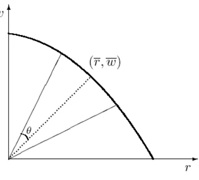
Now it is possible to represent graphically the relationship between the profit rate and the unit wage rate by means of the wage-profit frontier.
Fig.I.1 - Wage-profit frontier in the particular case of standard system
Fig.I.1 shows an example of the wage-profit frontier in a particular case, when the system considered is a standard system. The standard system and the standard commodity are two elements introduced by Sraffa in his search for an invariable measure of value. This search for an invariable measure of value was one of the most important problems posed by David Ricardo, but the English author was not able to find a solution. However, in order not to complicate the discussion, a more thorough description of these elements will be carried out in the next subsection. For the purposes of here is sufficient to recall that regardless of the fact that the production system is a standard system or not, the relationship between the unit wage rate and the profit rate is always strictly monotonic and thus the frontier is always descending and its intercept on the horizontal axis is R.
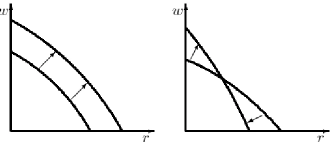
When a non-standard system is considered, the shape of the wage-profit frontier is no longer a straight line, but a complex path. This is due to the fact that when the system is non-standard prices change with the rate of profit and consequently the value of capital and the surplus also change. A further complication is that the shape of the wage-profit frontier is numéraire dependent.
R
w
I.2.1 The standard system and the standard commodity
One of the main research objectives of Sraffa was to identify an invariable measure of value that would allow isolating the price changes resulting from the characteristics of the commodities examined from those resulting from the characteristics of the commodity that is used as numéraire, by which the other relative prices are measured. In other words, it was shown above that there is a different price vector for each one of the infinite possible combinations of wages and profits. Consequently, it is useful to examine how the price of a particular commodity varies when the profit rate increases from zero to its maximum value.
However, since it is a relative price, its variation is caused by two factors: the first is the characteristics of the commodity itself, and then the intensity of capital used to produce it and the intensity of capital goods used in its production, the second is the characteristics of the commodity used as a numéraire that they may influence the relative price.
Therefore, Sraffa proposed the standard commodity as invariable measure of value. In order to uncover this commodity, Sraffa examines the effects of a change in the unit wage rate on the profit rate and the prices of the individual commodities, assuming that the production techniques remain unchanged.
When the entire surplus goes to wages relative prices are determined by the direct and indirect labor required to produce the commodities. This result sustains the labor theory of value supported by classical economists. However, when the rate of profit is positive, the labor theory of value is no longer valid and the key element in determining the movement of relative prices is given by the differences in the proportions of labor and capital that are used in various industries.
Nevertheless, the movement of relative prices depends not only on the proportion of labor and means of production of the commodity in question, but also on the relationship between labor and means of production of each of the other commodities used to produce it. A reduction of the unit wage rate produces a change in relative prices that rebalance the position of the industries in deficit, those with low labor-capital ratio, and the position of the industries in surplus, those with a relatively high labor-capital ratio.
The mathematical formalization of what has been said is now proposed following Pasinetti (1977).
Let us starts from usual price system
P⋅A⋅(1+r)+L⋅w = P (I.24)
which is a system with k equations and k +2 unknowns. To solve the system is necessary to fix the value of a distributional variable and select a numéraire.
which different commodities are produced are equal to the proportions in which they are used as inputs in the production.
P⋅(I – A) ⋅Q* = 1 (I.25)
where Q* is the column vector containing the total quantity of commodities produced by the standard system. Now it is important to note that the actual net product will be generally different from one, except at the point where the profit rate is zero. At this point, prices are proportional to the quantity of labor incorporated and the wage rate is exactly one9. The actual system (I.14) expressed in terms of standard commodity is thus as follows
P⋅A + P⋅A⋅r+L⋅w = P (I.26)
P⋅(I – A) ⋅Q* = 1 (I.27)
post-multiplying the members of the first equation and rearranging, we obtain
P⋅A⋅Q*⋅r = P⋅Q* - P⋅A⋅Q* - L⋅Q*⋅w = P (I.28)
P⋅A⋅Q*⋅r = P⋅ (I – A)⋅Q* - L⋅Q*⋅w = P (I.29)
Now, since P (I - A) Q * = 1 for (I.27) and L Q *= 1 by convention, we have then
P⋅A⋅Q*⋅r = 1 - w (I.30)
or multiplying both terms for the maximum rate of profit
P⋅A⋅Q*⋅r⋅R = R⋅ (1 – w) (I.31)
By isolating the term P A Q * R and by considering the equation of the standard system [I - (1 + R) A] Q *= 0, pre-multiplying by the prices and rearranging we have
P⋅A⋅Q*⋅ R = P⋅Q* - P⋅A⋅Q* (I.32)
P⋅A⋅Q*⋅ R = P⋅(I – A)⋅Q* (I.23)
9
Since P (I - A) Q *= 1, then P AQ * R = 1. Substituting in equation (I.21) yields
r = R⋅ (1 – w) (I.24)
which expresses the linear relationship between wages and the rate of profit. In conclusion then we can say that the complicated relationship between wages and the rate of profit, due to changes in the price components of the commodity used as numéraire, can be made linear by selecting the standard commodity as numéraire.
The linear relationship allows one to examine the income distribution between wages and profits, without its being subjected to distortions caused from price changes of the commodity used as numéraire.
I.2.2 The subsystems
Sraffa uses the notion of a subsystem to demonstrate that when the national income is entirely distributed to wages, the relative value of commodities is proportional to their respective labor costs. The description of the subsystems is introduced in Appendix A of Production of Commodities by means of Commodities (Sraffa, 1960, p.89).
The calculation of the subsystems from the original economic system can be made by adopting alternative methods, in what follows we will repropose the method used by Harcourt and Massaro (1964), because it explains in a clear and didactive way the process of decomposition.
Consider an economic system in which three industries produce the commodities a, b and c respectively:
(xaa⋅A⋅Pa+xab⋅A⋅Pb+xacA⋅Pc)⋅(1+r)+La⋅A⋅w = A⋅Pa (xba⋅B⋅Pa+xbb⋅B⋅Pb+xbc⋅B⋅Pc)⋅(1+r)+Lb⋅B⋅w = B⋅Pb (xca⋅C⋅Pa+xcb⋅C⋅Pb+xcc⋅C⋅Pc)⋅(1+r)+Lc⋅C⋅w = C⋅Pc
(I.25)
where r is the uniform rate of profit, w the unit wage rate, Pi the price of commodity i (i = a, b, c), xij is the input of commodity j required to produce one unit of output of commodity i ( i, j = a, b, c)¸ Li is the labor input per unit of commodity i (i = a, b, c), A, B, C are the total output of commodities a, b and c, respectively.
Table.I.1 – A production system with three commodities
MEANS OF PRODUCTION TOTAL OUTPUT
Industry Commodity Labor
a xaaA (+) xabA (+) xacA (+) laA xaaA xbaB xcaC Sa A
b xbaB (+) xbbB (+) xbcB (+) lbB xabA xbbB xcbC Sb B
c xcaC (+) xcbC (+) xccC (+) lcC xacA xbcB xccC Sc C
The net product components in physical terms are
Sa = A - α Sb = B – β Sc = C - γ
(I.26)
where
α = xaa⋅A + xba⋅B + xca⋅C
β = xab⋅A + xbb⋅B + xcb⋅C
γ = xac⋅A + xbc⋅B + xcc⋅C
(I.27)
The original system can now be divided into as many parts as there are commodities that make up the net product, so that each party is an autonomous self reproducing system with a net product consisting of a single commodity. Each part is called subsystem and in the example described here there are three subsystems.
The net products of each subsystem are equal to the amount of that commodity in net product of the original system. The total sum of each commodity used as means of production in the three subsystems is equal to their use as means of production in the original system. Similarly, the total labor employed in the three subsystems corresponds to that employed in the original system.
Tab. I.2 - Decompositions into subsystems of a production system with three commodities
MEANS OF PRODUCTION TOTAL OUTPUT
Industry Commodity Labor Industry Commodity Labor
a b c A
a
1a 1b 1c 1a
→
1a 1a 1a Sa 2a 2b 2c 2a 2a 2a 2a
3a 3b 3c 3a 3a 3a 3a
xaaA xabA xacA xaaA xbaB xcaC
MEANS OF PRODUCTION TOTAL OUTPUT
Industry Commodity Labor Industry Commodity Labor
a b c B
b
1a 1b 1c 1b
→
1b 1b 1b Sb 2a 2b 2c 2b 2b 2b 2b
3a 3b 3c 3b 3b 3b 3b
xbaB xbbB xbcB xabA xbbB xcbC
MEANS OF PRODUCTION TOTAL OUTPUT
Industry Commodity Labor Industry Commodity Labor
a b c C
c
1a 1b 1c 1c
→
1c 1c 1c Sc 2a 2b 2c 2c 2c 2c 2c
3a 3b 3c 3c 3c 3c 3c
xcaC xcbC xccC xacA xbcB xccC
Tab. I.3 - Subsystem 1
a 1a 1b 1c 1a → 1a 1a 1a
Sa
b 1a 1b 1c 1b → 1b 1b 1b
I.3 Structure of the thesis
The present work is organized in five chapters and it proposes and applies alternative measures of productivity constructed using input-output tables and based mainly on the Sraffian scheme. The first three chapters are self-contained, so they can be read independently, however they are of course thematically interrelated. The reading of chapter one is necessary for understanding chapters four and five.
The first three chapters of the thesis are devoted to the development and the empirical application of new productivity measures. These chapters form the main part of the work. The last two chapters are devoted to sensitivity analysis.
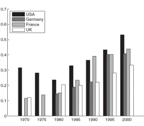
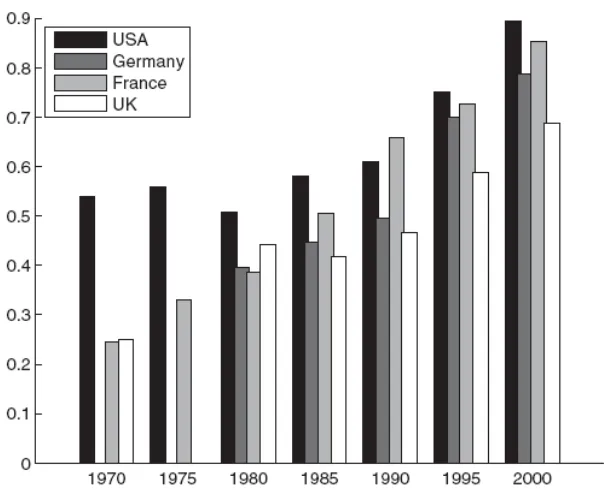
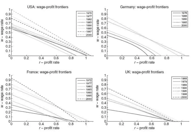
In the first chapter, entitled ‘Productivity accounting based on production prices’ an alternative method of productivity accounting is proposed. By using input–output tables from four major OECD countries between 1970 and 2000, we compute the associated wage-profit frontiers and the net national products curves, and from these we derive two measures of productivity growth based on production prices and a chosen numéraire. The findings support the general conclusions in the existing literature on the productivity slowdown and later rebound, and supply new important insights to the extent and timing of these events.
The second chapter is entitled ‘New measures of sectoral productivity’. The objective of this chapter is to propose alternative methods of sectoral productivity accounting based the theoretical work of Goodwin (1976), Gossling (1972), Pasinetti (1973), and Sraffa (1960). The indexes developed in this study differ from the standard indexes of productivity because they are designed on the basis of some of the following desiderable features: take into account the interconnections among economic sectors, aggregate heterogeneous goods by using production prices, and compute productivity by using quantity of goods instead of their values. These indexes are then be tested empirically by computing productivity of four major OECD countries.
Not surprisingly, analyses of the findings reveal that there is a productivity gap between the regions of North and South. However, the analysis of sectoral productivity reveals two important facts. The first is that the techniques of some industries are more productive in the South than in the North. The second, who follows from the first, is that all regions could therefore improve productivity through greater integration.
Chapter four is entitled ‘An Inquiry into the choice of Numéraire’. This chapter has several objectives. The main aim is to examine the robustness of the results obtained by applying the new approach to measuring productivity if we change the numéraire chosen. However, it should be mentioned that the problem of the choice of numéraire is a general one and for this reason, the chapter also proposes universal guidelines to be followed in choosing the numéraire and in testing the robustness of the results to changes in the numéraire.
Finally, chapter five is entitled ‘An Inquiry into the effect of aggregation of input-output tables’. The aim of this chapter is to test the robustness of the results from a progressive aggregation of the input-output tables.
I.4 Advantages of this approach to measuring
productivity
I.4.1 The rejection of the aggregate production function
The production function has been the subject of intense debate between the 50s and 70s during the so-called Cambridge-Cambridge controversy. Almost all the criticisms were directed at the aggregate production function, but also microeconomic production function has been put under scrutiny.
From the theoretical point of view, Felipe and Fisher (2003) showed that the conditions for which an aggregate function can be obtained by individual microeconomic functions are so stringent to be virtually impossible. For this reason, the aggregate production function does not have a sound theoretical foundation.
However, a number of empirical studies conducted up to early 70's showed that a production function of Cobb-Douglass type fit the data well and these results were used to justify the use of an aggregate production function.
In 1974, Shaikh proposed a critique of the neoclassical aggregate production function and its associated marginal-productivity theory of income distribution, by demonstrating that
change,” and “marginal products equal to factor rewards.” Since the above is a mathematical consequence of constant shares, true even for very implausible production data…
…it is argued that the so-called empirical strength of production function analysis is in reality nothing more that a statistical reflection of the (unexplained) constancy of income shares (Shaikh, 1974 p.119).
The Shaikh’s critique of the production function has continued over the years with a series of articles written by the same Shaikh, Felipe, McCombie, and others (see, among many, Shaikh 1980 and 2005, McCombie and Dixon 1991, Felipe and McCombie 2001, Fredholm 2009).
One of the main advantages of the aggregate and sectoral productivity measures proposed in this work is that they do not require any explicit assumption about the production function. In this way, the measures proposed here do not suffer the problems outlined above. Furthermore, the methods presented here do not suffer from the problem of aggregation of capital, which had also been the subject of intense debate during the Cambridge-Cambridge controversy (for an excellent concise survey on this topic see Pasinetti and Scazzieri, 2009).
I.4.2 The use of production prices
Many of aggregate and sectoral productivity measures presented in this work are constructed using prices of production. Thus, the approach followed here is that of the cost-of-production theory of value. This theory argues that the price of a commodity is determined by the cost of all the resources used to produce it. The prices of production are those at which the commodities must be sold in order to guarantee the reproducibility of the economic system. Hence, they differ from the market prices which are obtained by the conditions of supply and demand. The price of production of one commodity can be interpreted as a sign of the relative importance of that commodity for the economy as a whole, and therefore they represent a more appropriate weight for the aggregation of heterogeneous commodities.
I.4.3The scale invariance property of wage-profit frontier
concerning circulating capital only, sees Arrow, 1951; Koopmans, 1951; Samuelson, 1951).
The non-substitution theorem asserts that in a world with only one primary factor (labor) and without joint production, whatever are the possibilities of substitution between production factors, changes in demand imply no change in technical coefficients. The dual interpretation of the non-substitution theorem asserts that ‘under certain specified conditions an economy will have one particular price structure for each admissible value of the profit rate, regardless of the pattern of the final demand’ (Salvadori, 1987, p.680). It follows that for any kind of change in the scale of production, be it a change in the scale of production for the economy as a whole or a change in the scale of production that is asymmetric across industries, the invariance of the wage-profit frontier is by the non-substitution theorem guarantied in both cases.
Therefore, once a suitable numéraire has been selected, it is possible to compare wage-profit frontiers of very different countries and regions, and it is even possible to compare a large state with a small region, because the wage-profit frontier is determined by the technical condition of production and it does not depend on the size of the economy.
I.5 Limitations of this approach to measuring
productivity
I.5.1 The use of input-output tables in value-term
This work is mainly based on the application of the Sraffa’s model to input-output tables. The Sraffa’s scheme of production assumes that the physical commodities are produced through the use of physical commodities and labor, while the input-output tables currently available are expressed in value terms. Consequently, the application of the Sraffa model to input-output tables would not be legitimate. However, the use of input-output tables in a classical context à la Sraffa has some precedents in the literature (see Han and Schefold, 2006).
The hope is that in the near future may be available input-output tables whose values are expressed in physical quantities and with a high level of industry detail. In this way, it would be possible to match the theoretical model with the empirical application.
I.5.2 Fixed capital
production (see Sraffa, 1960 Ch.10). Unfortunately, the model of joint production leads to mathematical complications and the results are often of difficult economic interpretation.
However, there is an awareness of the need to improve the indicators proposed in this thesis, so that they can include fixed capital, but there is also awareness that the measurement of fixed capital stock is still problematic.
One of the most widely used methods for measuring the stock of capital is the Perpetual Inventory Method (PIM), but the PIM may frequently give inaccurate results due to inaccurate assumptions. In particular, it is not so easy to obtain precise and current information on the life span of different classes of asset. In an ideal situation of a totally stable economy, and limited technological change, provided the initial estimate of life spans was reasonably accurate, there would be no problem with PIM. But, that type of industrial environment does not exist, and never will. In practice actual asset lives change over time, and sometimes they change very rapidly.
I.5.3 The
numéraire
The problem of the choice of numéraire it is briefly introduced here for completeness, but this will be the subject of a more extended discussion in the next chapters. This is just to recall that the model of Sraffa consists of a system of linear equations with two more unknowns than equations. It is therefore necessary to fix the value of one of the two distributional variables and select a numéraire to find the solution. However, changes of the numéraire are not without consequences, because all the production prices will vary in a not predictable way.
I.6 Concluding remarks
A first consideration is that this thesis does not have the pretension to be exhaustive in such a large and complex argument. Rather, the aim is to provide “rules of thumb” for measuring productivity and technological progress in a more appropriate way than it is currently done.
I should say that this work is neither purely theoretical nor purely empirical. In this thesis the theory is used to construct indexes of productivity that are then applied to small samples of countries and regions. This work does not make any important theoretical contribution and empirical analysis is not conducted with excessive detail. Yet it is precisely this transition from theory to practice the real value added of the work.
References
Abramovitz M., (1956): ‘Resources and Output Trends in the United States since 1870.’ American Economic Review, 46, pp. 5.23.
Arrow K.J. (1951): ‘Alternative proof of the substitution theorem for Leontief models in the case of three industries’ in Activity Analysis of Production and Allocation, ed.T.C. Koopmans, New York, John Wiley.
Caves D.W., Christensen L.R., Diewert W.E. (1982a): ‘Multilateral comparison of output, input, and productivity using superlative index numbers.’ Economic Journal, 92, pp.73-89.
Caves D.W., Christensen L.R., Diewert W.E. (1982b): ‘The economic theory of index numbers and the measurement of input, output and productivity.’ Econometrica, 50, pp.1393-1414.
Charnes A., Cooper W., Rhodes E. (1978) ‘Measuring the efficiency of decision-making units’, European Journal of Operational Research, 2, pp. 429–444.
Denison E.F. (1972): ‘Some major issues in productivity analysis: An examination of the estimates by Jorgenson and Griliches’, Survey of Current Business, 49 (5, part 2), pp. 1–27.
Diewert W.E., Nakamura A.O., (1993): Essays in index number theory, North-Holland, Amsterdam.
Domar, Evsey (1946): ‘Capital Expansion, Rate of Growth and Employment’, Econometrica, 14, pp.137-147.
Eichhorn W., Voeller J. (1976): Theory of the Price Index: Fisher’s Text Approach and Generalizations, Lecture Notes in Economics and Mathematical Systems, Vol. 140, Berlin, Springer-Verlag.
Fare R., Grosskopf S., Norris M., Zhang Z. (1994):’Productivity growth, technical progress, and efficiency change in industrialized countries.’ American Economic Review, 84, pp.66-83.
Felipe J., Fisher F.M. (2003): ‘Aggregation in production functions: what applied economists should know’, Metroeconomica, 54, pp. 208 – 262.
Felipe J., McCombie J.S.L. (2001): ‘The CES production function, the accounting identity and Occam's razor’, Applied Economics, 33, pp. 1221 – 1232.
Fredholm T. (2009): ‘Production Functions Behaving Badly. Reconsidering Fisher and Shaikh’, Essay on the Theory of Production, Unpublished Ph.D. Thesis, Ch.4, University of Aalborg.
Fredholm T., Zambelli S. (2009): The Technological Frontier – An International and Inter-industrial Empirical Investigation of Efficiency, Technological Change, and Convergence, Fredholm T., unpublished Ph.D Thesis, Ch.3, University of Aalborg.
Goodwin R.M. (1976): ‘The use of normalized general coordinates in linear value and distribution theory’, in Polenske K.R. and Skolka J.V., Advances in Input-Output Analysis, Ballinger Publishing Company, Cambridge, MA.
Gossling W.F. (1972): Productivity Trends in a Sectoral Macro-economic Model, Input-Output Publishing CO., London.
Han Z., Schefold B. (2006): 'An empirical investigation of paradoxes: reswitching and reverse capital deepening in capital theory', Cambridge Journal of Economics, 30, pp. 737–765.
Harcourt G.C., Massaro V.G. (1964): ‘A Note on Mr.Sraffa’s Sub-Systems’, The Economic Journal, 74, 715-722.
Harrod Roy (1939): ‘An Essay in Dynamic Theory’, Economic Journal, LI, pp.14-33
Hulten C.R. (2000): ‘Total Factor Productivity: A Short Biography’, NBER Working Paper 7471, Cambridge, MA.
Jorgenson D. W. and Griliches, Z. (1967): ‘The Explanation of Productivity Change’, Review of Economic Studies, 34(3), pp. 249-83.
Jorgenson D. W. and Griliches, Z. (1972): ‘Issues in growth accounting: A reply to Edward F. Denison’, Survey of Current Business, 52, pp. 65–94.
Koopmans T.C., (1951): ‘Alternative proof of the substitution theorem for Leontief models in the case of three industries’ in Activity Analysis of Production and Allocation, ed.T.C. Koopmans, New York, John Wiley.Alternative
Laspeyres E. (1871): ‘Die Berechnung einer mittleren Waarenpreissteigerung’, Jahrbücher für Nationalökonomie und Statistik, 16, pp. 296-314.
Lovell C.A.L., Schmidt P. (1988): ‚A Comparison of Alternative Approaches to the Measurement of Productive Efficiency, in Dogramarici A., Fare R. (eds.) Applications of Modern Production Theory: Efficiency and Productivity, Kluwer, Boston.
McCombie J.S.L., Dixon R. (1991): ‘Estimating technical change in aggregate production functions: a critique’, International Review of Applied Economics, 5, pp. 24 – 46.
Neumann J. v. (1945–46): ‘A model o