On the Rate of Convergence of Regularized Boosting Classifiers

On the Rate of Convergence of Regularized Boosting Classifiers

Gilles Blanchard [email protected]

CNRS Laboratoire de Math´ematiques Universit´e Paris-Sud

Bˆatiment 425

91405 Orsay Cedex, France

G ´abor Lugosi [email protected]

Department of Economics, Pompeu Fabra University,

Ramon Trias Fargas 25-27, 08005 Barcelona, Spain

Nicolas Vayatis [email protected]

Universit´e Paris 6–Pierre et Marie Curie

Laboratoire de Probabilit´es et Mod`eles Al´eatoires 4, place Jussieu - Boite courrier 188

75252 Paris cedex 05, France

Editors: Thore Graepel and Ralf Herbrich

Abstract

A regularized boosting method is introduced, for which regularization is obtained through a pe-nalization function. It is shown through oracle inequalities that this method is model adaptive. The rate of convergence of the probability of misclassification is investigated. It is shown that for quite a large class of distributions, the probability of error converges to the Bayes risk at a rate faster than

n−(V+2)/(4(V+1))where V is theVCdimension of the “base” class whose elements are combined by boosting methods to obtain an aggregated classifier. The dimension-independent nature of the rates may partially explain the good behavior of these methods in practical problems. Under Tsybakov’s noise condition the rate of convergence is even faster. We investigate the conditions necessary to obtain such rates for different base classes. The special case of boosting using decision stumps is studied in detail. We characterize the class of classifiers realizable by aggregating decision stumps. It is shown that some versions of boosting work especially well in high-dimensional logistic addi-tive models. It appears that adding a limited labelling noise to the training data may in certain cases improve the convergence, as has been also suggested by other authors.

Keywords:classification, boosting, consistency, rates of convergence, decision stumps

1. Introduction

1998; Koltchinskii and Panchenko 2002). This view was complemented by Breiman’s observation (Breiman, 1998) that boosting performs gradient descent optimization of an empirical cost function different from the number of misclassified samples, see also Mason, Baxter, Bartlett, and Frean (1999), Collins, Schapire, and Singer (2000), Friedman, Hastie, and Tibshirani (2000). Based on this new view, various versions of boosting algorithms have been shown to be consistent in different settings, see Breiman (2000), B ¨uhlmann and Yu (2003), Jiang (2003), Lugosi and Vayatis (2003), Mannor and Meir (2001), Mannor, Meir, and Zhang (2002), Zhang (2003).

The purpose of this paper is a deeper investigation of the convergence of the probability of error of regularized boosting classifiers by deriving bounds for the rate of convergence. The main point is the introduction of a boosting procedure with regularization by a penalty function depending on the

`1norm of the boosting coefficients. The main result of the paper is an oracle inequality showing

that this procedure is model adaptive, and stating in particular that the rate of convergence for the probability of error of the associated classification rule converges to that of the Bayes classifier at a dimension-independent rate faster than n−(V+2)/(4(V+1))—where V is theVCdimension of the base classifiers—for a large class of distributions. The class of distributions for which this rate holds is defined in terms of properties of the function f∗minimizing the expected cost function. If the base classifier set is sufficiently rich, the class turns out to be quite large. The analysis also points out a curious behavior of boosting methods: in some cases the rate of convergence can be speeded up by adding (limited) random noise to the data!

We also note that under some additional natural assumption on the distribution, considered by Tsybakov (2003), Nedelec and Massart (2003), and Bartlett, Jordan, and McAuliffe (2003), the rate of convergence may be even faster.

One of the main objectives of this paper is to better understand the behavior of boosting methods using decision stumps. This special case is studied in detail first in a simple one-dimensional setting and then in general. We characterize the class of classifiers realizable by aggregating decision stumps. It is shown that some versions of boosting work especially well in high-dimensional logistic additive models in that they do not suffer from the “curse of dimensionality”.

consistent classification and have a fast rate of convergence for a large classes of distributions. We also emphasize the scale and rotation invariance of boosting methods based on several of these base classes. The proof of Theorem 1 is given in Section 7.

2. Setup

The binary classification problem we consider is described as follows. Let(X,Y)be a pair of random variables taking values in

X

×{−1,1}where

X

is a measurable feature space. Given a training data of n independent, identically distributed observation/label pairs Dn= (X1,Y1),...,(Xn,Yn), having

the same distribution as(X,Y), the problem is to design a classifier gn:

X

→ {−1,1}which assigns a label to each possible value of the observation. The loss of gnis measured by

L(gn) =P[gn(X)6=Y|Dn] .

The minimal possible probability of error is the Bayes risk, denoted by

L∗=inf

g L(g) =Emin(η(X),1−η(X))

where the infimum is taken over all measurable classifiers g :

X

→ {−1,1} and η(x) = P[Y = 1|X=x]denotes the posterior probability function. The infimum is achieved by the Bayes classifier g∗(x) =I_[η(x)>1/2]−I[η(x)≤1/2](whereIdenotes the indicator function).

The voting classifiers studied in this paper combine their decisions based on a weighted majority vote of classifiers from a base class of classifiers

C

, whose elements g :

X

→ {−1,1}of

C

are called the base classifiers. We denote theVCdimension of

C

by V and assume it is finite. For simplicity we assume that

C

is symmetric in the sense that for any g∈

C

we also have−g∈

C

. (This is equivalent to allowing negative weights in the voting schemes.)

We define by

F

λthe class of real-valued functions f :

X

→Robtained as nonnegative linear combinations of the classifiers in

C

with the sum of the coefficients equal toλ>0:

F

λ=

( f(x) =

N

∑

j=1

wjgj(x) : N∈N;∀1≤ j≤N,gj∈

C

,wj≥0 ; N

∑

j=1

wj=λ )

.

Note that the symmetry of

C

implies that

F

λ1 ⊂

F

λ2 whenever λ1<λ2. Each f ∈

F

λ defines a

classifier gf by

gf(x) =

1 if f(x)>0

−1 otherwise.

To simplify notation, we write L(f) =L(gf) =P[gf(X)6=Y]and

b Ln(f) =

1 n

n

∑

i=1

I_[gf(Xi)6=Yi].

To this end, letφ:R→R+be a twice differentiable, strictly increasing and strictly convex func-tion such thatφ(0) =1 and limx→−∞φ(x) =0 which we call the cost function. The corresponding risk functional and empirical risk functional are defined by

A(f) =Eφ(−Y f(X)) and An(f) =1 n

n

∑

i=1

φ(−Yif(Xi)).

We recall from Lugosi and Vayatis (2003) the simple fact that there exists an extended-real-valued function f∗minimizing A(f)over all measurable function, given by

f∗(x) =arg min

α∈R {η(x)φ(−α) + (1−η(x))φ(α)} .

We write A∗=A(f∗) =inffA(f).

The estimates we consider take the form

b

f_nλ=arg min f∈Fλ

An(f).

(Note that the minimum may not be achieved in

F

λ. However, to simplify the arguments we implic-itly assume that the minimum in fact exists. All proofs may be adjusted, in a straightforward way, to handle appropriate approximate minimizers of the empirical cost functional.) As argued in Lugosi and Vayatis (2003), the parameterλmay be regarded as a smoothing parameter. Large values ofλ improve the approximation properties of the class

F

λat the price of making the estimation problem

more difficult.

The estimators considered in this paper use a value of λchosen empirically, by minimizing a penalized value of the empirical cost An(bfnλ). To this end, consider a sequence of real numbers

(λk)k∈Nincreasing to+∞and letζ:R+→R+be a so-called penalty (or regularization) function. Define the penalized estimator by

b

fn=arg min k≥1

{An(bfnλk) +ζ(λk)}. (1)

The role of the penalty is to compensate for overfitting which helps find an adequate value ofλk. For larger values ofλk the class

F

λk is larger, and therefore ζ(λk)should be larger as well. By a

careful choice of the penalty, specified in Theorem 1 below, one may find a close-to-optimal balance between estimation and approximation errors.

The main purpose of this paper is to investigate the probability of error L(bfn)of the classifier g_bf

n induced by the penalized estimator. The decision function gbfn may be regarded as a regularized

boosting classifier where the regularization parameter λ controls the sum of the weights of the aggregated classifiers and is chosen by minimizing a penalized value of the empirical cost function.

Remark 1. Choosingλin a countable set is done here to simplify the proof of the oracle inequality in Theorem 1; the minimum overλ∈R+ could also be considered with similar results up to minor additional terms in the penalty.

of finite VC dimension may be replaced by the more general assumption that the covering num-bers

N

(ε,

C

,L2(Q))are bounded by cε−V for some positive constants c and V for any probability

distribution Q.

Remark 3. (COMPUTATIONAL ISSUES.) To compute the penalized estimator bfnin practice, one may proceed by computing, for eachλk, the minimizer bfλk

n of the empirical cost function. This may be done using iterative boosting algorithms which limit the sum of the weights of the base classifiers, such as MARGINBOOST.L1 proposed by Mason, Baxter, Bartlett, and Frean (1999). Furthermore,

many other algorithms have also been proposed to solve directly the regularized boosting problems of the type (1) when the minimization is performed over allλ>0. We refer the reader to the recent comprehensive review of Meir and R¨atsch (2003). For additional discussion on the algorithmic issues we refer to Bennett, Demiriz, and R¨atsch (2002), Lugosi and Vayatis (2003).

2.1 Relation to Earlier Work

Margin bounds. The first theoretical bounds about boosting-type methods are so-called “margin

bounds”. Although the motivation for deriving these bounds was initially to study the AdaBoost algorithm, these bounds are “agnostic” in the sense that they do not depend on the precise algo-rithm used, and can be applied for any algoalgo-rithm which returns an estimator belonging toS_λ>0

_F

_λ. These bounds rely on the complexity of the base class

C

and on an empirical quantity, called mar-gin. Schapire, Freund, Bartlett, and Lee (1998) proved the first bound of this type for boosting algorithms, and improved rates were obtained by Koltchinskii and Panchenko (2002). Duffy and Helmbold (2000) used the former result to study boosting-type algorithms with more general poten-tial functions (such as the functionφconsidered in this paper). Margin bounds provide an explicit confidence interval for the generalization error, although it is recognized that the bounds obtained are generally too loose to be of practical interest.

Oracle inequalities. As opposed to margin bounds, oracle-type inequalities refer to a precise

al-gorithm, usually some adaptive empirical loss minimization procedure over a family of models. Oracle inequalities ensure that the adaptive estimator does “almost” as well (up to additional terms that should be as small as possible) as the best possible function inside each model. Oracle inequal-ities do not provide an explicit confidence interval, but a guarantee about the performance and good behavior of the estimator with respect to a given collection of models. They allow, in particular, to derive bounds about convergence rates of the procedures considered. This type of bound will be our main focus in this paper.

Convergence rates and model adaptivity. An oracle inequality for the estimator defined by (1)

was derived by Lugosi and Vayatis (2003) (see also Zhang 2003 for oracle inequalities in a related but different framework), when the penalty function ζis of order n−1/2. However, it was proved by Bartlett, Jordan, and McAuliffe (2003) that, whenλis fixed, the rate of convergence of

A

(bf_nλ) towards inff∈FλA(f)is of order n−(V+2)/(2(V+1))—hence strictly smaller than O(n−1/2). This result

additional machinery and slightly different hypotheses for the model adaptive estimator. Additional discussion can be found in Section 7.

3. Main Results

To study the probability of error of the classifier g_bf

n, we first investigate the magnitude of A(bfn)−A

∗

which is well-known to be related to the difference L(bfn)−L∗. All subsequent results are based on the following theorem.

Theorem 1 Assume that the cost functionφis twice differentiable, strictly increasing and strictly convex withφ(0) =1 and limx→−∞φ(x) =0 such that the constant

L_φ=0∨max x∈R

2(φ0(x) +φ0(−x))

φ00

φ0(x) +φ 00

φ0(−x)

−(φ(x) +φ(−x)) !

(2)

is finite. (Here a∨b denotes the maximum of a and b.) Define

R(λ,n) = (V+2)VV++21((L_φ+2)φ(λ)) 1

V+1(λφ0(λ))

V V+1n−

1 2

V+2

V+1 ,

b(λ) = (Lφ+2)φ(λ),

and let(λk)k∈Nbe an increasing sequence in(1,+∞)such that∑k∈Nλ−αk ≤1 for someα>0. Then there exist positive constants c1,c2such that ifζ:R+→R+satisfies

∀λ>0, ζ(λ)≥c1R(λ,n) +

c2b(λ)(αlog(λ) +ξ+log(2))

n

for some positive numberξ, then, with probability at least 1−exp(−ξ), the penalized estimator bf defined by (1) satisfies

A(bfn)−A(f∗)≤2 inf k≥1

( inf f∈Fλk

(A(f)−A(f∗)) +2ζ(λk) )

.

The proof of this theorem is given in Section 7. A few remarks are in order.

Remark 1. (CONSTANTS.) Concrete values of the constants c1 and c2 may be obtained from the

proof. However, these values are not optimal and for clarity, and because our main focus here is on the rate of convergence as a function of the sample size, we preferred not to specify their values.

Remark 2. (CONFIDENCE.) The definition of the penalty given in the theorem depends on the confidence parameter ξ. However, note that its role is minor since it only appears in the smaller order second term. Indeed, for concreteness, one may take, for example,ξ=2 log n without altering the obtained rate of convergence. This choice also allows one to deduce “almost sure” convergence results by an application of the Borel-Cantelli lemma. The theorem presented here is derived as a consequence of Theorem 7 in Blanchard, Bousquet, and Massart (2003). (The statement of the cited result is given in Appendix A below.) It is also possible, with a penalty function of the same order up to logarithmic terms, to derive similar nonasymptotic upper bounds for the expected difference

Remark 3. (COST FUNCTIONS.) The properties required by Theorem 1 of the cost function are not claimed to be necessary to derive the result. Especially the condition involving the constant L_φ may seem unnatural, although it is not overly restrictive. In particular, the most widely used strictly convex cost functions, the exponential and the “logit” functions satisfy the property. Indeed, it is straightforward to check that forφ(x) =ex, Lφ=0 while for the logit cost φ=log₂(1+ex), L_φ=2−2 log 2. We give the corresponding explicit corollary for these two cost functions (using some straightforward upper bounds and the fact thatλ>1):

Corollary 2 For the exponential cost functionφ(x) =exp(x), the penalty function

ζ(λ) =c1(V+2)exp(λ)λ

V V+1_n−

1 2

V+2

V+1+_c2exp(λ)(αlogλ+ξ)

n ,

and for the logit costφ(x) =log(1+ex)the penalty function

ζ(λ) =c3(V+2)λn−

1 2

V+2

V+1+_c4λ(αlogλ+ξ)

n ,

(where c1,c2,c3,c4are appropriate constants) satisfy the requirements of Theorem 1.

In particular, for the logit cost, it is interesting to note that a penalization which behaves linearly (up to a logarithmic factor) inλis sufficient. This corresponds to a regularization function proportional to ||w||1, where w is the collection of coefficients defining a positive linear combination of base

class functions. This type of regularization has been proposed by various authors (see, e.g., Meir and R¨atsch 2003 for an overview).

How restrictive is condition (2) in the case of more general cost functions? Since we assumed that φis twice differentiable, strictly increasing and convex, Lφ is finite if and only if the limsup of the expression inside the maximum in (2), when x→ ±∞, is not+∞. A simple sufficient con-dition for this to hold is that there exists some L>0 such that lim infx→−∞(φ00/φ0)(x)>L and lim sup_x→+∞(φ0/φ)(x)<L/2. Furthermore, if we assume thatη(X)takes values in[ε,1−ε]almost surely, then by a straightforward modification of the proof of Theorem 1 (or, to be more precise, of Lemma 19 in Section 7) one sees that in the definition of L_φ, the maximum can be restricted to x∈[−f_ε∗,f_ε∗], where f_ε∗ is the value of f∗ at a point x such thatη(x) =1−ε. In this case Lφ is necessarily finite. Note that this assumption onηcan be enforced by adding a small flipping noise on the data labels (see the related discussion below).

We note that Bartlett, Jordan, and McAuliffe (2003) study the role of the cost function in depth and derive convergence results on a fixed model

F

λfor much more general cost functions. The more restrictive conditions needed here come from the fact that we consider an adaptive estimator over the set of models.

In the case when the distribution of the(X,Y)happens to be such that the “approximation error” inff∈FλkA(f)−A

∗_{vanishes for some value ofλ, the above theorem implies the following immediate}

corollary for the rate of convergence of A(bfn)to A∗.

Corollary 3 Assume that the distribution of (X,Y) is such that there exists a λ0>0 such that inff∈Fλ0A(f) =A(f∗). Under the conditions of Theorem 1, if the penalty is chosen to be

ζ(λ) =c1R(λ,n) +

c2b(λ)(αlog(λ) +2 log n+log 2)

then for every n, with probability at least 1−1/n2,

A(bfn)−A(f∗)≤Cn−12(

V+2

V+1)

where the constant C depends on the distribution, on the class

F

, and on the cost functionφ.

Note that the penalty function does not depend onλ0above, so that the procedure is truly adaptive. Of course, our main concern is not the behavior of the expected cost A(bfn)but the probability of error L(bfn)of the corresponding classifier. However for most cost functions the difference L(bfn)− L∗may directly be related to A(bfn)−A∗. Next we recall a simple but very useful inequality due to Zhang (2003). This result has been generalized to a great extent by Bartlett, Jordan, and McAuliffe (2003) for very general cost functions but we do not use the full power of their result.

Lemma 4 (ZHANG) Let φbe a nonnegative convex nondecreasing cost function such that there

exist constants c and s≥1 satisfying, for anyη∈[0,1],

1₂−ηs≤cs(1−H(η))

where H(η) =infα∈R(ηφ(−α) + (1−η)φ(α)). Then for any real-valued measurable function f ,

L(f)−L(f∗) ≤ 2c

Eh(1−H(η(X)))I_[g

f(X)6=g∗(X)]

i1/s

≤ 2c(A(f)−A(f∗))1/s.

We note here that for both the exponential and the logit cost functions the condition of the lemma is satisfied with c=√2 and s=2.

Lemma 4 implies that the rate of convergence of L(f)−L(f∗)to zero is at least as fast as the sth root of the rate of A(f)−A(f∗)to zero. The next lemma shows that, in fact, the excess probability of error L(f)−L(f∗)always goes to zero strictly faster than(A(f)−A(f∗))1/swhenever s is strictly greater than one. (Recall that this is the case for the exponential and logit cost functions that are our main concern in this paper.)

Lemma 5 Letφbe a nonnegative convex nondecreasing cost function such that there exist constants c and s>1 satisfying, for anyη∈[0,1],

1₂−ηs≤cs(1−H(η)).

Let{fn}be a sequence of real-valued measurable functions with limn→∞A(fn) =A(f∗). Then, as n→∞,

L(fn)−L(f∗)

(A(fn)−A(f∗))1/s →0.

PROOF. The proof is based on Lemma 4 and ideas from Devroye, Gy¨orfi, and Lugosi (1996, Theo-rem 6.5). Letε∈(0,1/2)be an arbitrary number. Then

= Eh|2η(X)−1|I_[g

fn(X)6=g∗(X)]

i

(see, e.g., Devroye, Gy¨orfi, and Lugosi 1996, Theorem 2.2)

= Eh|2η(X)−1|I_[g

fn(X)6=g∗(X)]I[|η(X)−1/2|≤ε]

i

+Eh|2η(X)−1|I_[g

fn(X)6=g∗(X)]I[|η(X)−1/2|>ε]

i

≤ Eh|2η(X)−1|sI_[g

fn(X)6=g∗(X)]

i1/s

· P

gfn(X)6=g

∗_{(X),|η(X)−1/2| ≤ε,η(X)6=}1

2

₍s−1)/s

+P[gfn(X)6=g

∗_{(X),|η(X)−1/2|>ε]}(s−1)/s !

(by H ¨older’s inequality applied for both terms)

Using the assumption onφ,

Eh|2η(X)−1|sI_[g

fn(X)6=g∗(X)]

i

≤ (2c)sE h

(1−H(η(X)))I_[g

fn(X)6=g∗(X)]

i

≤ (2c)s(A(fn)−A(f))

by Lemma 4. Thus, it suffices to prove that the sum of the two probabilities above may be made arbitrarily small for large n, by an appropriate choice ofε. To this end, first note that for any fixedε,

lim

n→∞P[gfn(X)6=g

∗_{(X),|η(X)−1/2|>ε] =0}

because otherwise L(fn)−L(f∗) would not converge to zero, contradicting the assumption that A(fn)−A(f∗)converges to zero (by Lemma 4). On the other hand,

P

gfn(X)6=g∗(X),|η(X)−1/2| ≤ε,η(X)6=

1 2

≤P

|η(X)−1/2| ≤ε,η(X)6=1 2

which converges to zero asε→0, and the proof is complete.

Thus, when s>1, L(fn)−L(f∗)converges to zero faster than(A(fn)−A(f∗))1/sfor all distri-butions. However, to obtain nontrivial bounds for the ratio of these two quantities, one has to impose some assumptions on the underlying distribution. This may be done by following Tsybakov (2003) who pointed out that under certain low-noise assumptions on the distribution much faster rates of convergence may be achieved. Tsybakov’s condition requires that there exist constantsα∈[0,1] andβ>0 such that for any real-valued measurable function f ,

P[gf(X)6=g∗(X)]≤β(L(f)−L∗)α . (3)

Lemma 6 (BARTLETT, JORDAN, AND McAULIFFE) Letφbe a cost function satisfying the condi-tions of Lemma 4 and assume that condition (3) holds for someα∈[0,1]andβ>0. Then

L(f)−L(f∗)≤

2sc

β1−s(A(f)−A(f

∗₎₎1/(s−sα+α) _.

For the cost functions that are most important for the present paper, s=2 and in that case, asα moves from zero to one, the exponent 1/(s−sα+α)changes from 1/2 to 1. Thus, large values of

αsignificantly improve the rates of convergence of L(f)to L∗.

Combining Corollary 3 with Lemmas 4, 5, and 6 we obtain the following result. Even though it may be generalized trivially for other cost functions, for concreteness and simplicity we only state it for the two cost functions that have been most important in various versions of boosting classifiers. Recall that for both of these cost functions the condition of Lemma 4 is satisfied with s=2.

Corollary 7 Letφbe either the exponential or the logit cost function and consider the penalized estimate bfnof Corollary 3. Assume that the distribution of(X,Y)is such that there exists aλ>0 such that inff∈FλA(f) =A(f∗). Then for every n, with probability at least 1−1/n2, the probability

of error L(bfn)of the associated classifier satisfies

L(bfn)−L∗≤Cn−

1 4(VV++21)

where the constant C depends on the distribution, on the class

F

, and on the cost functionφ. Also, with probability one,

lim n→∞

L(bfn)−L∗

n14(

V+2

V+1) =₀.

If, in addition, condition (3) holds for some α∈[0,1] and β>0, then with probability at least 1−1/n2,

L(bfn)−L∗≤Cn−

1 2(2−α)(

V+2

V+1) .

Corollary 7 is the main result of this paper on which the rest of the discussion is based. The remarkable fact about this corollary is that the obtained rate of convergence is independent of the dimension of the space in which the observations take their values. The rates depend on the VC

dimension of the base class which may be related to the dimension of the input space. However, this dependence is mild and even if V is very large, the rates are always faster than n−1/(2(2−α)). In the rest of the paper we consider concrete examples of base classes and argue that the class of dis-tributions for which such surprisingly fast rates can be achieved can be quite large. The dependence on the dimension is mostly reflected in the value of the constant C. Recall from Theorem 1 that the value of C is determined by the smallest value ofλfor which inff∈FλA(f) =A(f∗)and its

depen-dence onλis determined by the cost functionφ. For complex distributions, high-dimensional input spaces, and simple base classes, this constant will be very large. The main message of Corollary 7 is that, as a function of the sample size n, the probability of error converges at a fast rate, independently of the dimension. To understand the meaning of this result, we need to study the main condition on the distribution, that is, that the minimizer f∗of the expected cost falls in the closure of

F

λ(in the

sense that inff∈FλA(f) =A(f∗)) for some finite value ofλ. In the next sections we consider several

Remark. (APPROXIMATION ERROR). In Corollary 7 we only consider the case where inff∈FλA(f) =A(f∗)for some finite value ofλ. In this paper we focus on this simplest situation and

try to understand the nature of the distributions satisfying such conditions. On the other hand, under general conditions it can be guaranteed that the approximation error inff∈FλA(f)−A(f∗)converges

to zero asλ→∞, see, for example, Lugosi and Vayatis (2003), and Section 6 of the present paper. In this case Theorem 1 implies that A(bfn)→A(f∗)with probability one, so that the procedure is always consistent (thus improving the results of Lugosi and Vayatis (2003) since the penalty we consider in the present paper is of strictly smaller order in n). Furthermore, Theorem 1 tells us more: the penalized procedure effectively finds a tradeoff between the approximation properties of the sets

F

λand the estimation error. A precise study of these approximation properties and of the corresponding rates of convergence is a complex, important, and largely unexplored problem.

4. Decision Stumps on the Real Line

In this section we consider the simple one-dimensional case when

X

= [0,1]and when the base class contains all classifiers g of the form g(x) =st+(x) =I[x≥t]−I[x<t] and of the form g(x) =s−t (x) =

I[x<t]−I[x≥t]where t∈[0,1]can take any value. (We note here that all results of this section may be extended, in a straightforward way, to the case when

X

=Rby the scale invariance of the estimates we consider.) Clearly, theVCdimension of

C

is V =2. In order to apply Corollary 7 it remains to describe the class of distributions satisfying its conditions. The next lemma states a simple sufficient condition.

Lemma 8 Assume that the cost function and the distribution of(X,Y)are such that the function f∗ is of bounded variation. If| · |BV denotes the total variation, define|f|BV,0,1= 1₂(f∗(0) +f∗(1) + |f∗|BV). Then inff∈FλA(f) =A(f∗)wheneverλ≥ |f∗|BV,0,1.

PROOF. Assume that f∗has a bounded variation. Then f∗may be written as a sum of a nondecreas-ing and a nonincreasnondecreas-ing function. A nondecreasnondecreas-ing function h on[0,1]may be approximated by a finite mixture of stumps as follows. Denote C=h(1)−h(0). Let N be a positive integer and let t1,...,tN be 1/N,...,N/N-quantiles of h, that is, ti=sup{x : h(x)<h(1)i/N}, i=1,...,N. Then

the function

e

h(x) =h(0) + N

∑

i=1

C

NI[x≥ti]=

h(1) +h(0)

2 s

+ 0(x) +

N

∑

i=1

C 2Ns

+

ti(x)

is at most C/N away from h in the supremum norm. Note also that eh∈

F

|h|BV,0,1. Similarly, a

nonincreasing function g may be approximated by a functioneg∈

_F

_|g|BV,0,1 such that sup_x∈[0,1]|g(x)− e

g(x)| ≤(g(0)−g(1))/N. Thus, the function ef =eh+eg is such that

sup x∈[0,1]

|f∗(x)−ef(x)| ≤ h(1)−h(0) +g(0)−g(1)

N =

|f∗|BV N

and moreover ef ∈

F

|f∗|BV,0,1 since |h|BV+|g|BV =|f∗|BV. Thus, since N is arbitrary, f∗ is in the

closure of

F

|f∗|BV,0,1 with respect to the supremum norm. The statement now follows by the continuity

ofφand the boundedness of the functions in the closure of

F

|f∗|BV,0,1 with respect to the supremum

Thus, the fast rates of convergence stated in Corollary 7 can be guaranteed whenever f∗ is everywhere finite and has a bounded variation. Recall that for the exponential cost function f∗=

(1/2)log(η/(1−η))and for the logit cost function f∗=log(η/(1−η)). In both cases, it is easy to see that f∗has a bounded variation if and only ifηis bounded away from zero and one and has a bounded variation. In particular, we obtain the following corollary matching the minimax rate of convergence for the probability of error obtained with a different method by Yang (1999a).

Corollary 9 Let X∈[0,1]. Letφbe either the exponential or the logit cost function and consider the penalized estimate bfnof Corollary 3 based on decision stumps on the real line. If there exists a constant b>0 such that b≤η(X)≤1−b with probability one andηhas a bounded variation, then for every n, with probability at least 1−1/n2, the probability of error L(bfn)of the associated classifier satisfies

L(bfn)−L∗≤Cn−13

where the constant C depends on b and|η|BV. Also, with probability one,

lim n→∞n

1 3

L(bfn)−L∗

=0.

If, in addition, condition (3) holds for someα∈[0,1]andβ>0, then for every n, with probability at least 1−1/n2,

L(bfn)−L∗≤Cn−

2 3(2−α) .

The dependence of the value of the constant C on b and|η|BV may be determined in a straight-forward way from Theorem 1. If λk is the smallest value for which inff∈FλkA(f) =A

∗_{, then the}

constant C in the first inequality is proportional to (Lφ+2)φ(λk) 1

6(λ

kφ0(λk))

1

3_{. Clearly,}λ

kcan be bounded as a function of b and|η|BV as shown in Lemma 8. Concrete values are given in Corollary 12 below in the more general multivariate case.

The condition thatη(x)is bounded away from zero and one may seem to be quite unnatural at first sight. Indeed, values ofη(x)close to zero and one mean that the distribution has little noise and should make the classification problem easier. However, regularized boosting methods suffer when faced with a low-noise distribution since very large values ofλ are required to drive the approx-imation error inff∈FλA(f)−A∗ close to zero. (Note, however, that even whenηdoes not satisfy

the conditions of Corollary 9, limn→∞L(bfn) =L∗almost surely, under a denseness assumption, by Corollary 7.) The next simple example illustrates in part that phenomenon: indeed, ifλis not suffi-ciently large to make

F

λcontain f∗, then the classifier minimizing A(f)over

F

λmay indeed have a

very large probability of error because the function minimizing the A-risk puts all its mass on points for whichηis close to 0 or 1, while “neglecting” other points.

Example 1. (MINIMIZING A COST FUNCTION FOR A FIXEDλMAY BE BAD.) This example shows a situation in which ifλis not large enough, even though the class

F

λcontains a function f such that the corresponding classifier gf equals the Bayes classifier g∗, the function f_λ minimizing the expected cost A(f)over

F

λinduces a classifier with a significantly larger probability of error.

Consider a simple problem where the distribution of X is atomic, distributed uniformly on the four points x1,...,x4. The base class

C

contains five classifiers: for each i=1,...,4 there is a

gi(x) =2I_[x=xi]−1 and also

C

contains the trivial classifier g0(x)≡1. Obviously, for anyλ>0,

consider the distribution defined byη(x1) =1/2+δ,η(x2) =1/2−δ, η(x3) =1, andη(x4) =0.

Then it is easy to show that ifφis a convex strictly increasing differentiable cost function andλ0 is such thatφ0(−λ0) =2δ, then for anyλ≤λ0, the optimizer of the cost function f_λputs positive weight on x3and x4and zero weight on x1and x2and thus has a probability of error L(gf_λ) =1/4 while the Bayes error is L∗=1/4−δ/2. The details of the proof are given in Appendix B. Note that the fact thatηis 1 and 0 on x3and x4is only to make the example simpler; we could assume η(x3) =1/2+∆,η(x4) =1/2−∆with∆>δand observe a comparable behavior.

Ifηcan be arbitrarily close to 0 and 1, then f∗takes arbitrarily large positive or negative values and thus cannot be in any

F

λ (since functions in this set take values in [−λ,λ]). However, one may easily force the condition of Corollary 9 to hold by adding some random noise to the data. Indeed, if, for example, we define the random variable Y0 such that it equals Y with probability 3/4 and−Y with probability 1/4, then the functionη0(x) =P[Y0=1|X =x] =1/4+η(x)/2 takes its values in the interval [1/4,3/4] (a similar transformation was also proposed by Yang 1999a, Yang 1999b). More importantly, the Bayes classifier g0 for the distribution(X,Y0)coincides with the Bayes classifier g∗ of the original problem. Also, recalling from Devroye, Gy¨orfi, and Lugosi (1996) that for any classifier g,

L(g)−L∗=EI_[g(X)6=g∗(X)]|2η(X)−1|

and denoting the probability of error of g under the distribution of(X,Y0)by L0(g)and the corre-sponding Bayes error by L0∗, we see that for any classifier g,

L(g)−L∗=2(L0(g)−L0∗). (4)

This means that if one can design a classifier which performs well for the “noisy” problem(X,Y0), then the same classifier will also work well for the original problem(X,Y). Thus, in order to enlarge the class of distributions for which the fast rates of convergence guaranteed by Corollary 9 holds, one may artificially corrupt the data by a random noise, replacing each label Yi by a noisy version Y_i0 as described above. Then the distribution of the noisy data is such that η0(x) is bounded away from zero. If we also observe that|η0|BV = (1/2)|η|BV and that if η(x) satisfies condition (3) for some α∈[0,1]and β>0 thenη0(x) also satisfies condition (3) with the sameα∈[0,1]but with

β0₌₂α_{β, we obtain the following corollary.}

Corollary 10 Let X∈[0,1]. Letφbe either the exponential or the logit cost function and consider the penalized estimate bfnbased on decision stumps, calculated based on the noise-corrupted data set described above. If η(x) has a bounded variation, then for every n, with probability at least 1−1/n2, the probability of error L(bfn)of the associated classifier satisfies

L(bfn)−L∗≤Cn−

1 3

where the constant C depends only on|η|BV. If, in addition, condition (3) holds for someα∈[0,1] andβ>0, then

L(bfn)−L∗≤Cn−3(2−α2 ) .

sped up considerably for some distributions. (Indeed, this fact was already pointed out by Yang in establishing general minimax rates of convergence in various settings (see Yang 1999a, Yang 1999b).) Besides, recall that, in the case we consider a cost functionφsuch that the constant L_φis infinite in Equation (2), Theorem 1 cannot be applied in general; however since the noise-degraded

η0 _{is bounded away from 0 and 1, Lφ can be replaced by some finite constant (see the remark}

about cost functions following Theorem 1), and hence Theorem 1 can be applied for the noisy distribution. For many distributions, the performance deteriorates by adding noise, but at least the rate of convergence is guaranteed to stay the same, and only the value of the constant C will be affected. Unfortunately, it is impossible to test whether ηis bounded away from zero or not, and it may be safe to add a little noise. Of course, the level of the added noise (i.e., the probability of flipping the labels in the training set) does not need to be the 1/4 described above. Any strictly positive value may be used and Corollary 10 remains true. While a more precise study is out of the scope of this paper, let us just remark that a sensible choice of the noise level based on the present bounds should be able to find a tradeoff between the improvement of the bias in the A-risk and the performance degradation as appearing in Equation (4).

Finally, a natural question is whether the improved convergence rate that could be obtained by adding a small labelling noise to the training data really is a practical consequence of using a “surrogate” convex loss (the function φ) instead of the 0−1 loss, or if it is just an artefact of the analysis. Namely, consider a case where the data is completely separable with some marginθ>0 by some function f ∈

F

1. In this situation the margin bounds of Koltchinskii and Panchenko (2002)

ensure that the convergence rates are as fast as in our analysis, and no labelling noise is needed. However, in a generic situation the problem with using the surrogate A-risk is the disequilibrium between regions where the target function f∗is very large or even infinite, and other regions where it is relatively small (of course in such a situation the data is not separable). In this situation, it may very well happen that the estimator will tend to concentrate all of its efforts on the former regions while neglecting the latter, as was shown prototypically in Example 1. Then, adding a small amount of noise could effectively bring the estimator to improve on the latter regions, which would have a definite effect on generalization error. Whether adding noise artificially is helpful in practice should be investigated by an adequate experimental study.

5. Decision Stumps in Higher Dimensions

5.1 Stumps and Generalized Additive Models

In this section we investigate the case when

X

= [0,1]d and the base class

C

contains all “decision stumps”, that is, all classifiers of the form s+_i,t(x) =I_[x(i)_≥t]−I[_x(i)_<t]and s−_i,_t(x) =I[_x(i)_<t]−I[_x(i)_≥t],

t∈[0,1], i=1,...,d, where x(i)denotes the i-th coordinate of x.

An important property of boosting using decision stumps is that of scale invariance. Indeed, if each component of the observation vectors Xi is transformed by a (possibly different) strictly monotone transformation then the resulting classifier does not change. This remark also implies that the assumption that the observations take their values from the bounded set[0,1]d is not essential, we use it for convenience.

A straightforward extension of the proof of Lemma 8 in the previous section shows that the closure of

F

λwith respect to the supremum norm contains all functions f of the form

where the functions fi:[0,1]→Rare such that|f1|BV,0,1+···+|fd|BV,0,1≤λ. Therefore, if f∗has

the above form, we have inff∈FλA(f) =A(f∗).

Recalling that the function f∗optimizing the cost A(f)has the form

f∗(x) =1 2log

η(x) 1−η(x)

in the case of the exponential cost function and

f∗(x) =log η(x) 1−η(x)

in the case of the logit cost function, we see that boosting using decision stumps is especially well fitted to the so-called additive logistic model in whichηis assumed to be such that log(η/(1−η)) is an additive function (i.e., it can be written as a sum of univariate functions of the components of x), see Hastie and Tibshirani (1990). The fact that boosting is intimately connected with additive logistic models of classification has already been pointed out by Friedman, Hastie, and Tibshirani (2000). The next result shows that indeed, whenηpermits an additive logistic representation then the rate of convergence of the regularized boosting classifier is fast and has a very mild dependence on the distribution.

Corollary 11 Let X ∈[0,1]d with d≥2. Letφbe either the exponential or the logit cost function and consider the penalized estimate bfnof Corollary 3 based on decision stumps. Let V2=3, V3=

4,V4=5, and for d≥5, Vd=b2 log2(2d)c. If there exist functions f1,...,fn:[0,1]→Rof bounded variation such that log_1−η(η(x)_x)=∑d_i=1fi(x(i))then for every n, with probability at least 1−1/n2, the probability of error L(bfn)of the associated classifier satisfies

L(bfn)−L∗≤Cn−

1 4

Vd+2

Vd+1

where the constant C depends on∑d_i=1|fi|BV,0,1. If, in addition, condition (3) holds for someα∈[0,1]

andβ>0, then

L(bfn)−L∗≤Cn−

1 2(2−α)

Vd+2

Vd+1

.

PROOF. The statements follow from Corollary 7. The only detail that remains to be checked is the

VC dimension Vd of the class

C

of decision stumps. This may be bounded by observing that the shatter coefficient (i.e., the maximum number of different ways n points in[0,1]d can be classified using decision stumps) is at most min(2d(n+1),2n). Thus, for d≥5, 2d(n+1)<2nif and only if n>log₂(2d)+log₂(n+1)which is implied by n>2 log₂(2d). For d≤4, just notice that decisions stumps are linear splits and theVCdimension of the class of all linear splits inRdequals d+1.

Remark. (DEPENDENCE ON THE DIMENSION.) Under the assumption of the additive logistic model, the rate of convergence is of the order of n(2(2−α))−1(Vd+2/Vd+1)_{where Vd depends on d in a}

logarithmic fashion. Even for large values of d, the rate is always faster than n−1/2(2−α). It is also useful to examine the dependence of the constant C on the dimension. A quick look at Theorem 1 reveals that C in the first inequality of Corollary 11 may be bounded by a universal constant times p

take λ=∑d_i=1|fi|BV,0,1. Since Vd =b2 log2(2d)c, the dependence on the dimension is primarily

determined by the growth of the cost functionφ. Here there is a significant difference between the behavior of the exponential and the logistic cost functions in high dimensions. For the purpose of comparison, it is reasonable to consider distributions such that λ=∑d_i=1|fi|BV,0,1 is bounded

by a linear function of d. In that case the constant C depends on d as O(pded_{log d}) _{in the case} of the exponential cost function, but only as O(√d log d) in the case of the logistic cost function (using directly Theorem 1 instead of the upper bound mentioned above). In summary, regularized boosting using the logistic cost function and decision stumps has a remarkably good behavior under the additive logistic model in high dimensional problems, as stated in the next corollary.

Corollary 12 Let X∈[0,1]d with d≥2. Letφbe the logit cost function and consider the penalized estimate bfn of Corollary 3 based on decision stumps. Let B be a positive constant. If there exist functions f1,...,fn:[0,1]→R with λ=∑di=1|fi|BV,0,1 ≤Bd such that log_1−η(η(x)_x) =∑di=1fi(x(i)) then for every n, with probability at least 1−1/n2_{, the probability of error L(}b_f

n)of the associated classifier satisfies

L(bfn)−L∗≤C p

d log d n−

1 4

Vd+2

Vd+1

where C is a universal constant and Vdis as in Corollary 11. If, in addition, condition (3) holds for someα∈[0,1]andβ>0, then

L(bfn)−L∗≤C(d log d)

1 2−α _n−

1 2(2−α)

Vd+2

Vd+1

.

Remark 1. (ADDING NOISE.) Just like in the one-dimensional case, the conditions of Corollary 11 require thatηbe bounded away from zero and one. To relax this assumption, one may try to add random noise to the data, just like in the one-dimensional case. However, this may not work in the higher-dimensional problem because even if f∗is an additive function, it may not have this property any longer after the noise is added.

Remark 2. (CONSISTENCY.) The results obtained in this paper (for instance, Corollary 7) imply the consistency of the classifier bfn under the only assumption that f∗ may be written as a sum of functions of the components, that is, that L(bf)→L∗ almost surely. The additional assumption on the bounded variation of the components guarantees the fast rates of convergence. However, if f∗is not an additive function, consistency cannot be guaranteed, and the example of the previous section shows that boosting is not robust in the sense that it is not even guaranteed to perform nearly as well as the best classifier contained in the class. Still, it is important to understand the structure of the classifiers that can be realized by aggregating decision stumps. The rest of this section is dedicated to this problem.

5.2 Set Approximation Properties of Mixtures of Stumps

In what follows we investigate what kind of sets A⊂[0,1]d can be well approximated by sets of the form Af ={x|f(x)>0}, where f ∈

F

λis a linear combination of decision stumps.

00 00 00

11 11 11

000 000 000

111 111 111

x

y

z w

0000 0000 0000 0000

1111 1111 1111 1111

00000 00000 00000 00000

11111 11111 11111 111110000

0000 0000 0000

1111 1111 1111 1111

?

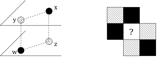
Figure 1: Points or regions belonging to the set A are in black. Left: four points inXORposition. Right: a counterexample to Theorem 14 when_X is not a cube: if the center square is not part of_X, the non-XORrequirement is satisfied, but any way to “extend”_X and A to the center square will lead to a creation of anXORposition.

Next consider the case d=2. It is then easy to see that if a set A is obtained as the support of the positive part of an additive function of the form f(x) = f1(x(1)) +f2(x(1)) then there cannot exist

four points x,y,z,w, such that these points are the corners of a rectangle aligned with the axes, the two corners on one diagonal are elements of A, and the two points of the other diagonal are not in A. We call this the “XOR” position. It turns out that this simple property, which we call for brevity the “non-XOR requirement”, is actually a necessary and sufficient condition for a set to be of the form

Af for f ∈

F

λfor anyλ>0.

Next we generalize this idea to d-dimensions and characterize completely the sets one can obtain with the additive models in the discrete setting. For this we need a more general definition of the

XORposition (see also Figure 1).

Definition 13 Let

X

={0,1/k,... ,k/k}d and A⊂

X

. We say that four points x,y,z,w are inXOR

position with respect to A if there exists an 1≤i0≤d such that

(

x(i0)=_y(i0), _z(i0)=_w(i0)_;

x(i)=z(i), y(i)=w(i),for i6=i0;

(5)

and x,w∈A but y,z6∈A.

For a discrete grid we have the following characterization of sets realizable as the positive part of the mixture of stumps. Recall that a set S is called a monotone layer inRd if it has one of the following properties: either (1) for any x∈S all points y≤x are also in S, or (2) for any x∈S all points y≥x are also in S. (We say that y≤x if the inequality holds componentwise.)

Theorem 14 Let

X

={0,1/k,... ,k/k}d and A⊂

X

. The following properties are equivalent: (i) There exists f such that A={x|f(x)>0}where f(x) = f1(x(1)) +...+fd(x(d));

(ii) There does not exist any x,y,z,w∈

X

inXORposition with respect to A;

PROOF. (i) ⇒ (ii): consider four points x,y,z,w satisfying (5). Suppose that x,w∈A and y6∈A, which means f(x),f(w)>0, f(y)≤0. Note that condition (i) and (5) imply that f(x) +f(w) =

f(y) +f(z). Hence we must have f(z)>0 and the points cannot be inXORposition.

(ii) ⇒ (iii): consider “slices” of X perpendicular to the first coordinate axis, that is, S_i1=

x∈

X

|x(1)=i/k . Define an order on the slices by saying that S1_i S1_j if and only if for any x= (i/k,x2,...,xd)∈S1i, if we denote y= (j/k,x2,...,xd)∈S1j, thenI[A(x)]≤I[A(y)]. Now, note that (ii) implies that this order is total, that is, for any i,j either S1_i S1_j or S1_j S_i1. As a consequence, we can rearrange the order along the first coordinate using a permutationσ1, so that the slices are sorted in increasing order. By doing this we do not alter the non-XORproperty, hence we can repeat the corresponding procedure along all the other coordinates. It is then easy to see that the image of A by these successive reorderings is now a monotone layer.

(iii)⇒(i): first note that any monotone layer can be represented as a set of the form described in (i). Therefore, any set obtained from a monotone layer by permutations of the order along each of the axes can also be represented under this form, since it is just a matter of accordingly rearranging, separately, the values of f1,...,fd.

Note that it is essential in the last theorem that

X

is an hypercube[0,1]d. In Figure 1 we show a contrived counterexample where

X

is not a cube and satisfies condition (ii) of the above theorem; yet it is not possible in this case to find a function f satisfying (i), because there is no way to “complete” the middle square so that the non-XOR requirement is still satisfied.

In the general case when

X

= [0,1]d, we can derive, based on the discrete case, an approximation result for sets whose boundary is of measure zero. The approximation is understood in the sense of L1 distance between indicators of sets with respect to the probability measure of X on

X

(or, equivalently, the measure of the symmetric difference of the sets). Note that this distance is always at least as large as the excess classification error.

Theorem 15 Let A⊂

X

be a set whose boundaryδA is of measure zero. Suppose there do not exist four points x,y,z,w∈

X

in XOR position with respect to A. Then there exists a sequence (fn)of linear combinations of decision stumps such that

lim

n→∞P[|I[fn(X)>0]−I[X∈A]|]→0.

PROOF. We approximate

X

by discrete grids. Fix some n∈Nand for I= (i1,...,id)∈ {0,...,n−1}d

denote xI= (i1/n,...,id/n)and let B(I)be the closed box xI+ [0,1]d. Let∆nbe the set of indices I such that B(I)contains at least a point of the boundary of A, and Bn=∪I∈∆nB(I).

Now consider the discrete set

Xn

=nxI,I∈ {0,...,n−1}d o

and the projection An=A∩

Xn.

Now in

Xn

, Ansatisfies the hypothesis (ii) of Theorem 14, and hence (i) is satisfied as well and there exists a function fn(x) = fn_,1(x(1))+...+fn,d(x(d))defined for x∈

Xn

with An={x∈

Xn

|f(x)>0}. Extend the functions fn_,jon[0,1]by defining (with some abuse of notation) fn,j(i/n+ε) = fn,j(i/n) forε∈(0,1/n). Obviously, the extended functions fn,jare still mixtures of stumps.

Let now gn(x) =I_[fn(x)>0],x∈

X

. We have gn(x) =I[A(x)] for x6∈Bn, by construction, and

therefore

P[|I[fn(X)>0]−I[X∈A]|]≤P[X∈Bn],

Remark. (DISREGARDING THE BOUNDARY.) Since we concentrate on sets A with boundary of measure 0, it is equivalent in the sense of the L1distance between sets to consider A, its closure A or its interior int(A). One could therefore change the above theorem by stating that it is sufficient that the “non-XORrequirement” be satisfied by some set C such that int(A)⊂C⊂A. It would be even nicer, if only of side interest, only to take into account quadruples of points not on the boundary of A to satisfy the non-XOR requirement, so that any problem arising with the boundary may be disregarded. In Appendix C we show that this is actually the case whenever P(δA) =0 for some measure P having full support, e.g., the Lebesgue measure).

The theorems above help understand the structure of classifiers that can be realized by a linear combination of decision stumps. However, for boosting to be successful it is not enough that the Bayes classifier g∗can be written in such a form. It may happen that even though g∗is in the class of classifiers induced by functions in

F

λ, the classifier corresponding to f_λminimizing the cost A(f) in

F

λis very different. This is the message of Example 1 above. The next example shows a similar situation in which for anyλ>0 there exists an f ∈

F

λsuch that gf =g∗.

Example 2. (BAYES CLASSIFIER MAY BE DIFFERENT FROM THE ONE CHOSEN BY BOOSTING.) Consider a two-dimensional problem with only two non-trivial classifiers in

C

given by two linear separators, one vertical and one horizontal, and the trivial classifier assigning−1 to everything. We have four regions (denoted D1 D2

D3 D4

) and only three parameters (only one parameter per classifier including the trivial one). By considering only symmetric situations whereηis the same on D1and

D4, we see that f , the function minimizing A(f)over

S

λ>0

F

λ, must also be symmetric and hence

we reduce (after re-parameterization) to two parameters a,b. The minimizer f is then of the form f=

(a+b)/2 a b (a+b)/2

.

First consider a situation in which X falls in D1or D4with probability zero. Then in this case

f= f∗ on D2 and D3. Furthermore, by choosingηsuitably in these regions, one may assume that

a>0>b but a+b>0. Now suppose that we put a tiny positive weightεon regions D1and D4,

with the Bayes classifier on these regions being class−1. But by continuity, the associated f_ε will stay positive on these regions ifεis small enough. Then g_f

ε6=g∗on these regions, while obviously

for anyλ>0 we can find an appropriate function f ∈M_λsuch that gf =g∗= −₋₁1 1₋₁

in this case.

6. Examples of Consistent Base Classes

The results of the previous section show that using decision stumps as base classifiers may work very well under certain distributions such as additive logistic models but may fail if the distribution is not of the desired form. Thus, it may be desirable to use larger classes of base classifiers in order to widen the class of distributions for which good performance is guaranteed. Recent results on the consistency of boosting methods (see, e.g., Breiman 2000, B ¨uhlmann and Yu 2003, Jiang 2003, Lugosi and Vayatis 2003, Mannor and Meir 2001, Mannor, Meir, and Zhang 2002, Zhang 2003) show that universal consistency of regularized boosting methods may be guaranteed whenever the base class is so that the class of linear combinations of base classifiers is rich enough so that every measurable function can be approximated. In this section we consider a few simple choices of base classes satisfying this richness property. In particular, we recall here the following result (Lugosi and Vayatis, 2003, Lemma 1):

Lemma 16 (LUGOSI AND VAYATIS) Let the class

C

be such that its convex hull

F

1 contains all

generates

B

(Rd_{). Then}

lim

λ→∞f∈λ·infF1

A(f) =A∗.

More generally, a straightforward modification of this Lemma shows that whenever

F

=Sλ>0

F

λ

is dense in L1(µ), then it is true that inff∈FA(f) =A(f∗).

We consider the following examples; in all cases we assume that

X

=Rd_.

(1)

C

lin contains all linear classifiers, that is, functions of the form g(x) =2I_[a·x≤b]−1, a∈Rd, b∈R.

(2)

C

rectcontains classifiers of the form g(x) =2I[x∈R]−1 where R is either a closed rectangle or its complement inRd.

(3)

C

ball contains classifiers of the form g(x) =2I_[x∈B]−1 where B is either a closed ball or its complement inRd.

(4)

C

ell contains classifiers of the form g(x) =2I_[x∈E]−1 where either E a closed ellipsoid or its complement inRd.

(5)

C

treecontains decision tree classifiers using axis parallel cuts with d+1 terminal nodes.

Clearly, the list of possibilities is endless, and these five examples are just some of the most natural choices. All five examples are such that S_λ>0

F

λ is dense in L1(µ) for any probability

distribution µ (In the cases of

C

rect,

C

ball, and

C

ell this statement is obvious. For

C

lin this follows

from denseness results of neural networks, see Cybenko 1989, Hornik, Stinchcombe, and White 1989. For

C

tree, see Breiman 2000.) (We also refer to the general statement given as a universal

approximation theorem by Zhang 2003 and which shows that, for the classical choices of the cost functionφ, we have, for any distribution, inff∈S_λ>0FλA(f) =A∗as soon as

S

λ>0

F

λis dense in the

space of continuous functions under the supremum norm.) In particular, the results in the present paper imply that in all cases, the penalized estimate bfnof Corollary 3 is universally consistent, that is, L(bfn)→L∗almost surely as n→∞.

Recall that the rates of convergence established in Corollary 7 depend primarily on the VC

dimension of the base class. The VCdimension equals V =d+1 in the case of

C

lin, V =2d+1

for

C

rect, V=d+2 for

C

ball, and is bounded by V =d(d+1)/2+2 for

C

ell and by V=d log2(2d)

for

C

tree (see, e.g., Devroye, Gy¨orfi, and Lugosi, 1996). Clearly, the lower the VC dimension is,

the faster the rate (estimation is easier). The following question arises naturally: find a class with VC dimension as small as possible whose convex hull is sufficiently rich in L1(µ). A recent result

by Lugosi and Mendelson (2003) establishes the existence of such a class with VC dimension at most 2. This fact reveals that the combinatorial complexity of a class is not always a reliable measure of the approximation capacity of its convex hull. However, the construction by Lugosi and Mendelson is theoretical and there is probably more to say if one is concerned with practical implementations of boosting methods (see also Remark 1 below). In all cases, for even moderately large values of d, the rate of convergence stated in Corollary 7 is just slightly faster than n−1/(2(2−α)), and the most interesting problem is to determine the class of distributions for which inff∈FλA(f) =