Schultz and Modified Schultz Polynomials of Cog-Complete Bipartite Graphs

http://www.sciencepublishinggroup.com/j/acm doi: 10.11648/j.acm.20170606.14

ISSN: 2328-5605 (Print); ISSN: 2328-5613 (Online)

Schultz and Modified Schultz Polynomials of Cog-Complete

Bipartite Graphs

Ahmed Mohammed Ali, Haitham Nashwan Mohammed

Department of Mathematics, College of Computer Sciences and Mathematics, University of Mosul, Mosul, Iraq

Email address:

[email protected] (A. M. Ali), [email protected] (H. N. Mohammed)

To cite this article:

Ahmed Mohammed Ali, Haitham Nashwan Mohammed. Schultz and Modified Schultz Polynomials of Cog-Complete Bipartite Graphs.

Applied and Computational Mathematics. Vol. 6, No. 6, 2017, pp. 259-264. doi: 10.11648/j.acm.20170606.14

Received: September 9, 2017; Accepted: November 9, 2017; Published: December 18, 2017

Abstract:

Let G be a simple connected graph, the vertex- set and edge- set of G are denoted by V(G) and E(G), respectively. The molecular graph G, the vertices represent atoms and the edges represent bonds. In graph theory, we have many invariant polynomials and many invariant indices of a connected graph G. Topological indices based on the distance between the vertices of a connected graph are widely used in theoretical chemistry to establish relation between the structure and the properties of molecules. The coefficients of polynomials are also important in the knowledge some properties in application chemistry. The Schultz and modified Schultz polynomials, Schultz and modified Schultz indices and average distance of Schultz and modified Schultz of Cog-complete bipartite graphs are obtained in this paper.

Keywords:

Schultz and Modified Schultz Polynomials, Cog-Complete Bipartite Graphs, Topological Indices, Boundary Average Distance

1. Introduction

Suppose that = ( ( , ( is a simple undirected connected graph of order = ( and size = ( . A graph G is called an n-partite graph, ≥ 2, if it possible to partition vertex– set ( in to non empty subsets

, , … , (called partite sets) such that every element of

( joins a vertex of V to a vertex of V, for all r ≠ t for

n = 2, such graphs are called bipartite graphs. A complete bipartite graph G is a 2- partite graph with petite sets V and

V having the added property that if ∈ and ∈ , then

∈ ( with two partite sets V and V denoted by K _, (or K(m, n , where |V | = m and |V | = n. The distance between any two vertices u and v of G is the length of a shortest (u,v)-path in a connected graph G, denoted by

( , . In particular, if = , then ( , = 0 . Topological indices in biology and chemistry was used for the first time in 1947 when chemist Harold Wiener [1] introduced Wiener index to demonstrate correlations between physicochemical properties of organic compounds of molecular graphs. TheWiener index is represent the total distance of a connected graph G, i.e.

"( = ∑$,%∈&(' ( , , in which the summation is taken

over all unordered pairs { , } of distinct vertices of G. The

diameter of G is the greatest distance in G and will be denoted by *. The number of pairs of vertices of G that are distance k is denoted by ( , + . Distance is an important concept in graph theory and it has applications to computer science, chemistry, and a variety of other fields [2-6].

For the definitions of concepts and notations used in this papers, vertices with distance k such that |,-( | = ( , . and ∑2_-3 ( , . = /01, where /01 is representation the number of unordered pairs of distinct vertices in G.

In chemical graph theory, there are two important polynomials are distinguished. Introduced:

The Schultz polynomial of a graph G is defined as:

45( ; 7 = ∑_$,%∈&('(*$+ *% 79($,% _,

and modified Schultz polynomial of a graph G is defined as:

45∗_{( ; 7 = ∑$,%∈&('(*$*% 7}9($,% _.

These based structure descriptors and their polynomials were extensively studied and computed before [7-9].

The Schultz index is defined as:

45( = ∑$,%∈&('(*$+ *% ( , ,

and modified Schulttz index is defined as:

45∗_{( = ∑ (*$*% ( ,}

$,%∈&(' .

where the summation for all above are taken over all unordered pairs of distinct vertices in V(G).

The indices of Schultz and modified Schultz can be obtained by the derivative of Schultz and modified Schultz polynomials with respect to x at x = 1, respectively, i.e.:

45( =_9A9 45( ; 7 B_A3 , and 45∗( =_9A9 45∗( ; 7 B

A3 .

The average distance of a connected graph G with respect Schultz and modified Schultz are defined as:

45( = 45( //01, and 45∗( = 45∗( //01.

In 2005, Gutman find many relations between Hosoya, Schultz and modified Schultz polynomials of a tree graph and some properties [12]. Bo Zhou [13], find some lower and upper bounds for the Schultz index of a graph G.

The Schultz and modified Schultz polynomial of some special graphs are summarized in the following theorem (See [14]). In addition, we have found the Schultz and modified Schultz polynomials of some Cog- special graphs which it under publication.

In 2013, Hassani et al. computed the Schultz polynomials of isomeres of C _EE Fullerene by GAP program [15].

The Schultz indices have been shown to be a useful molecular descriptors in the design of molecules with desired properties, reader can be see the papers [16-18].

Finally, Farahani found Schultz and modified Schultz polynomials and topological indices of benzene molecules PAHs, coronene polycyclic aromatic hydro carbons and some Haray graphs [8, 19, 20] in 2017, Guo and Zhow studies the propeties of degree distance and Gutman index of uniform hypergraphs [21].

2. Main Results

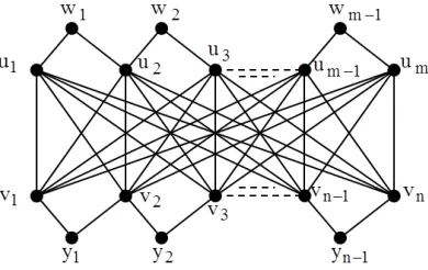
Definition: A Cog- complete bipartite graph +F,G is the graphconstructedfrombipartitecompletegraph +F, , H, ≥ 2, of vertices set {u , u , … , u , v , v , … , v } with H + − 2 of additional vertices {K , K , . . . , KFM , N , N , . . . , N _M }, and

2m+2n−4 of additional edges {KP P, KP PQ : S = 1,2, … , H −

1} ∪ {NP P, NP PQ : S = 1,2, … , − 1}, see Figure 1.

Figure 1. A Cog- complete bipartite graph +_F,G .

From Clearly that /+F,G 1 = 2H + 2 − 2, /+F,G 1 =

H( + 2 + 2( − 2 and * = SVH+F,G = 4, for all

H, ≥ 4.

Theorem 2.1:For all H, ≥ 4, then

45/+F,G _{; 71 = {H (H + + 8 + 4(H + − 5 }7 + 2{H ( + 1 + ( − 4 ( + 1 + H( + 3 ( − 1 }7 +} {H ( + 4 + H( − 2 − 16 + 4( − 4 + 7 }7\_{+ 2{H(H − 5 + ( − 5 + 12}7}]_{. (1)} 45∗_/+F,G _{; 71 = {H (H + 2H + 2 + 8 − 20}7 + {H (H + (7H/2 + (7 /2 − 4 + 2H(H − 4 + 2 ( − 4 +}

2}7 + 2{H ( + 2 + (H + 2 − 2(H + 4H + 4 − 9 }7\_{+ 2{H(H − 5 + ( − 5 + 12}7}]_{. (2)}

Proof: For all vertices _ _ ∈ /+_F,G 1, there is (_ , _ = ., . = 1,2,3,4. From clearly that ∑ |,P| = (2H + 2 − 3 (H + − 1]_P3 .

We will have four partitions for proof:

P1. If (_ , _ = 1, then |D | = m(n + 2 + 2(n − 2 and is equal to /+F,G 1, we have ten subsets of it:

P1.1. Ba/u ₍ , w _{( M} 1: δd_e(f + δg_e(fhe = n + 3 & δd_e(fδg_e(fhe = 2(n + 1 jB = 2.

P1.2. kl(wm, umQ : δg_n+ δd_noe= n + 4 & δg_nδd_noe= 2(n + 2 , 1 ≤ i ≤ m − 2rk = m − 2.

P1.3. kl(wm, um : δg_n+ δd_n= n + 4 & δg_nδd_n= 2(n + 2 , 2 ≤ i ≤ m − 1rk = m − 2.

P1.4. Ba/v₍ , y _{( M} 1: δt_e(u + δv_e(uhe = m + 3 & δt_e(uδv_e(uhe = 2(m + 1 jB = 2.

P1.5. kl(ym, vmQ : δv_n+ δt_noe = m + 4 & δv_nδt_noe = 2(m + 2 , 1 ≤ i ≤ n − 2rk = n − 2.

P1.7. Ba/um, vw1: δd_n+ δt_x = m + n + 2 & δd_nδt_x= (m + 1 (n + 1 , i = 1, m, j = 1, njB = 4.

P1.8. Ba/um, vw1: δd_n+ δt_x= m + n + 3 & δd_nδt_x= (m + 1 (n + 2 , 2 ≤ i ≤ m − 1, j = 1, njB = 2(m − 2 .

P1.9. Ba/um, vw1: δd_n+ δt_x = m + n + 3 & δd_nδt_x = (m + 2 (n + 1 , i = 1, m, 2 ≤ j ≤ n − 1jB = 2(n − 2 .

P1.10. Ba/um, vw1: δd_n+ δt_x= m + n + 4 & δd_nδt_x= (m + 2 (n + 2 , 2 ≤ i ≤ m − 1, 2 ≤ j ≤ n − 1jB = (m − 2 (n − 2 .

P2. If (_ , _ = 2, then |D | = (4mn + m(m − 1 + n(n − 1 − 8 /2, we have twelvesubsets of it:

P2.1. kl(ym, ymQ : δv_n+ δv_noe = 4 & δv_nδv_noe = 4, 1 ≤ i ≤ n − 2rk = n − 2.

P2.2. kl(wm, wmQ : δg_n+ δg_noe = 4 & δg_nδg_noe = 4, 1 ≤ i ≤ m − 2rk = m − 2.

P2.3. kl(v , v : δt_e+ δt_u= 2(m + 1 & δt_eδt_u= (m + 1 rk = 1.

P2.4. Ba/vm, vw1: δt_n+ δt_x = 2m + 3 & δt_nδt_x = (m + 1 (m + 2 , i = 1, n, 2 ≤ j ≤ n − 1jB = 2(n − 2 .

P2.5. Ba/vm, vw1: δt_n+ δt_x = 2(m + 2 & δt_nδt_x = (m + 2 , 2 ≤ i ≤ n − 2, i + 1 ≤ j ≤ n − 1jB = (n − 2 (n − 3 /2.

P2.6. kl(u , u : δd_e+ δd_f = 2(n + 1 & δd_eδd_f= (n + 1 rk = 1.

P2.7. Ba/um, uw1: δd_n+ δd_x = 2n + 3 &δd_nδd_x = (n + 1 (n + 2 , i = 1, m, 2 ≤ j ≤ m − 1jB = 2(m − 2 .

P2.8. Ba/um, uw1: δd_n+ δd_x= 2(n + 2 & δd_nδd_x = (n + 2 , 2 ≤ i ≤ m − 2, i + 1 ≤ j ≤ m − 1jB = (m − 2 (m − 3 /2.

P2.9. Ba/vm, ww1: δt_n+ δg_x= m + 3 &δt_nδg_x= 2(m + 1 , i = 1, n, 1 ≤ j ≤ m − 1jB = 2(m − 1

P2.10. Ba/vm, ww1: δt_n+ δg_x = m + 4& δt_nδg_x = 2(m + 2 , 2 ≤ i ≤ n − 1, 1 ≤ j ≤ m − 1jB = (m − 1 (n − 2 .

P2.11. Ba/um, yw1: δd_n+ δv_x = n + 3 & δd_nδv_x= 2(n + 1 , i = 1, m, 1 ≤ j ≤ n − 1jB = 2(n − 1 .

P2.12. Ba/um, yw1: δd_n+ δv_x= n + 4 & δd_nδv_x= 2(n + 2 , 2 ≤ i ≤ m − 1, 1 ≤ j ≤ n − 1jB = (m − 2 (n − 1 .

P3. If (_ , _ = 3, then |D_\| = mn + m(m − 4 + n(n − 4 + 5, we have seven subsets of it:

P3.1. Ba/u , ww1: δd_e+ δg_x= n + 3 & δd_eδg_x= 2(n + 1 , 2 ≤ j ≤ m − 1jB = m − 2.

P3.2. Ba/u , ww1: δd_f+ δg_x= n + 3 & δd_fδg_x = 2(n + 1 , 1 ≤ j ≤ m − 2jB = m − 2.

P3.3. Ba/um, ww1: δd_n+ δg_x= n + 4 & δd_nδg_x= 2(n + 2 , 2 ≤ i ≤ m − 1,1 ≤ j ≤ m − 1, |i − j| ≠ 0,1jB = (m − 2 (m − 3 .

P3.4. Ba/v , yw1: δt_e+ δv_x= m + 3 &δt_eδv_x = 2(m + 1 , 2 ≤ j ≤ n − 1jB = n − 2.

P3.5. kl(v , ym : δt_u+ δv_n= m + 3 &δt_uδv_n= 2(m + 1 , 1 ≤ i ≤ n − 2rk = n − 2.

P3.6. Ba/vm, yw1: δt_n+ δv_x= m + 4 &δt_nδv_x= 2(m + 2 , 2 ≤ i ≤ n − 1, 1 ≤ j ≤ n − 1, |i − j| ≠ 0,1jB = (n − 2 (n − 3 .

P3.7. Ba/wm, yw1: δg_n+ δv_x = 4 & δg_nδv_x= 4,1 ≤ i ≤ m − 1, 1 ≤ j ≤ n − 1jB = (m − 1 (n − 1 .

P4. If (_ , _ = 4, then |,\| = (H(H − 5 + ( − 5 + 12 /2, we have two subsets of it:

P4.1. Ba/wm, ww1: δg_n+ δg_x = 4 & δg_nδg_x= 4,1 ≤ i ≤ m − 3, i + 2 ≤ j ≤ m − 1jB = (m − 2 (m − 3 /2.

From P1-P4 and after the computational processes we get the two equations (1) and (2). Corollary 2.2: For all H, ≥ 4, then

45/+F,G 1 = 8H ( + 3 + 8 (H + 3 + 10H − 96(H + + 144. (3) 45∗_/+F,G _{1 = 3H (H − 8 + 3H (5 + 8 + 3 (5H + 8 − 104(H + + 188. (4)}

Proof:

To get equations (3) and (4), we derivative the equations (1) and (2) with respect to 7 and then compensation of the value of

7 by 1.

Corollary 2.3: For all H, ≥ 4, then

1. 45(+F,G = (8H ( + 3 + 8 (H + 3 + 10H − 96(H + + 144 /(H + − 1 (2H + 2 − 3 .

2. 45∗/+F,G 1 = (3H (H − 8 + 3H (5 + 8 + 3 (5H + 8 − 104(H + + 188 /(H + − 1 (2H + 2 − 3 . Proof: obvious

Corollary 2.4: For all H = ≥ 4, then

45/+F,G ; 71 = 2(H\+ 4H + 4H − 10 7 + 4(H\+ 2H − 3H − 2 7 + 2(H\+ 3H − 16H + 14 7\+ 4(H − 3 (H − 2 7]. (5)

45∗_/+F,G _{; 71 = (H}]_{+ 4H}\_{+ 8H − 20 7 + (H}]_{+ 7H}\_{− 16H + 2 7 + 4(H}\_{− 8H + 9 7}\_{+ 4(H − 3 (H − 2 7}]_{. (6)}

Proof: from possible to obtain formulas (5) and (6) from formulas (1) and (2) by equality , H (H = and after simplified processes.

Corollary 2.5: For all H = ≥ 4, then

1. 45/+F,G 1 = 16H\+ 58H − 192H + 144.

2. 45∗/+F,G 1 = 3H]+ 30H\+ 24H − 208H + 188. Proof: similar to proof corollary 2.2.

Corollary 2.6: For all H = ≥ 4, then 1. 14.5 < 45(+_F,G < 2H + 10.

2. 26.7 < 45∗(+_F,G < 3(4H + 45H + 87 /32.

When = 2 and = 3 for all H ≥ 4, we obtain the same formulas in the Theorem 2.1 and corollary 2.2 after off setting the value = 2 and = 3 for all H ≥ 4, in the Theorem 2.1 and corollary 2.2 respectively.

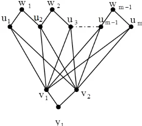
As special case, if = 2, H ≥ 4, then +F,G is shown in Figure 2.

Figure 2. A Cog- complete bipartite graph +_F,G .

Theorem 2.7: For H ≥ 4, then

45/+F,G ; 71 = 2(H + 12H − 6 7 + 2(3H + 5H − 6 7 + 2(3H − 8H + 6 7\+ 2(H − 3 (H − 2 7]. (7) 45∗_/+F,G _{; 71 = 4(2H + 6H − 5 7 + (13H − 2H − 6 7 + 4(2H − 6H + 5 7}\_{+ 2(H − 3 (H − 2 7}]_{. (8)}

Proof: For every vertices _ _ ∈ (+F,G , there is d(z1,z2)=k, k=1,2,3,4, and obvious ∑ |,P| = (2H + 1 (H + 1]P3 .

We will have four partitions for proof:

P1. If (_ , _ = 1, then |D | = 4m and is equal to /+F,G 1, we have six subsets of it:

P1.1. Ba/u ₍ , w _{( M} 1:δ_de(f +δ_ge(fhe = 5 & δ_de(fδ_ge(fhe = 6jB = 2.

P1.2. kl(wm, um :δ_gn+δ_dn = 6 & δ_gnδ_dn= 8, 2 ≤ i ≤ m − 1rk = m − 2.

P1.3. kl(wm, umQ :δ_gn+δ_dnoe = 6 & δ_gnδ_dnoe = 8, 1 ≤ i ≤ m − 2rk = m − 2.

P1.4. Ba/um, vw1:δ_dn+δ_tx = m + 4 & δ_dnδ_tx= 3(m + 1 , i = 1, m, j = 1,2jB = 4.

P1.5. Ba/um, vw1:δ_dn+δ_tx= m + 5 & δ_dnδ_tx= 4(m + 1 , 2 ≤≤ m − 1, j = 1,2jB = 2(m − 2 .

P1.6. kl(y , vm :δ_ve+δ_tn = m + 3 & δ_veδ_tn = 2(m + 2 , i = 1,2rk = 2.

P2.1. kl(wm, wmQ :δ_gn+δ_gnoe = 4 & δ_gnδ_gnoe = 4, 1 ≤ i ≤ m − 2rk = m − 2.

P2.2. Ba/vm, ww1:δ_tn+δ_gx = m + 3 & δ_tnδ_gx = 2(m + 1 , i = 1,2, 1 ≤ j ≤ m − 1jB = 2(m − 1 .

P2.3. kl(um, y :δ_dn+δ_ve = 5 & δ_dnδ_ve = 6, i = 1,2rk = 2.

P2.4. kl(um, y :δ_dn+δ_ve= 6 & δ_dnδ_ve = 8,2 ≤ i ≤ m − 1rk = m − 2.

P2.5. kl(u , u :δ_de+δ_df = 6 & δ_deδ_df= 9rk = 1.

P2.6. Ba/um, uw1:δ_dn+δ_dx = 7 & δ_dnδ_dx= 12,2 ≤ i ≤ m − 1, j = 1, mjB = 2(m − 2 .

P2.7. Ba/um, uw1:δ_dn+δ_dx= 8 & δ_dnδ_dx = 16,2 ≤ i ≤ m − 2, i + 1 ≤ j ≤ m − 1jB = (m − 2 (m − 3 /2.

P2.8. kl(v , v :δ_te+δ_tz= 2(m + 1 & δ_teδ_tz = (m + 1 rk = 1.

P3. If (_ , _ = 3, then|D_\| = (m − 1 , we have four subsets of it:

P3.1. kl(y , wm :δ_ve+δ_gn= 4 & δ_veδ_gn= 4,1 ≤ i ≤ m − 1rk = m − 1.

P3.2. kl(u , wm :δ_de+δ_gn= 5 & δ_deδ_gn = 6,2 ≤ i ≤ m − 1rk = m − 2.

P3.3. kl(u , wm :δ_df+δ_gn= 5 & δ_dfδ_gn= 6,1 ≤ i ≤ m − 2rk = m − 2.

P3.4. Ba/um, ww1:δ_dn+δ_gx= 6 & δ_dnδ_gx= 8,2 ≤ i ≤ m − 1, 1 ≤ j ≤ m − 1, |i − j| ≠ 0,1jB = (m − 2 (m − 3 .

P4. If(_ , _ = 4, then |,\| = ((H − 2 + (H − 3 + 12 /2, we have:

Ba/wm, ww1:δ_gn+δ_gx = 4 & δ_gnδ_gx= 4,1 ≤ i ≤ m − 3, i + 2 ≤ j ≤ m − 1jB = (m − 2 (m − 3 /2

From P1-P4 and after the computational processes we get the two equations (7) and (8). Also we can obtain the same formula when compensating the value of n by 2 in the Theorem 2.1.

Corollary 2.8: For H ≥ 4, we have: 1. 45/+F,G 1 = 4(10H − 11H + 12 . 2. 45∗/+F,G 1 = 2(33H − 46H + 38 . Corollary 2.9: For H ≥ 4, we have: 1. 11.3 < 45(+_F,G < 20.

2. 16.9 < 45∗(+_F,G < 33.

Theorem 2.10: For H ≥ 4, we have:

1. 45/+F,\G ; 71 = (3H + 37H − 8 7 + (8H + 24H −

8 7 + (7H − 13H + 16 7\_{+ (2H − 10H + 12 7}]_.

2. 45∗/+_F,\G ; 71 = (15H + 42H − 20 7 + {(43H + 23H −

8 /2}7 + (10H − 22H + 24 7\_{+ (2H − 10H + 12 7}]_.

Proof: By the same way proof the Theorem 2.1. Corollary 2.11: For H ≥ 4, we have:

1. 45/+F,\G 1 = 48H + 6H + 72. 2. 45∗/+F,\G 1 = 96H − 41H + 92. Corollary 2.12: For H ≥ 4, we have: 1. 14 < 45/+_F,\G 1 < 24.

2. 25 < 45∗/+_F,\G 1 < 48. Remark:

1. 45/+G_, ; 71 = 447 + 327 + 47\.

45/+\,G ; 71 = 787 + 727 + 187\.

45/+\,\G _{; 71 = 1307 + 1367 + 407}\_.

2. 45∗/+G_, ; 71 = 607 + 427 + 47\.

45∗_/+\,G _{; 71 = 1247 + 1057 + 207}\_. 45∗_/+\,\G _{; 71 = 2417 + 2247 + 487}\_.

3. Conclusion

In this paper we managed to find the Schultz and modified Schultz polynomials and Schultz and modified Schultz indices of Cog- complete bipartite graph +F,G of order

2H + 2H − 2, H, ≥ 2. Also, we given the boundary lower and upper of average distance of Schultz and modified Schultz of Cog- complete bipartite graph +F,G .

References

[1] Wiener, H.; (1947), “StructuralDeterminationof Paraffin Boil- ing Points” J. Amer. Chem. Soc., 69, 17-20.

[2] Diudea, M. V. (ed.); (2001). QSPR/QSAR Studies by Molecular Descriptors, Nova, Huntington, New York. [3] Diudea, M. V., Gutman, I. and J¨antschi, L.; (2001). Molecular

Topology, Nova, Huntington, New York.

[5] Devillers, J. and Balaban, A. T. (eds.); (1999). Topological Indices and Related Descriptors in QSAR and QSPR, Gordon & Breach, Amsterdam.

[6] Diestel, R.; (2000). Graph Theory, electronic ed., Springer- Verlag, New York.

[7] Farahaini M. R., (2013); "Hosoya, Schultz Modified Schultz Polynomials and their Topological Indices of Benzene Molecules: First Members of polycyclic Aromatic Hydro Carbons (PAHs)"; International Journal of theoretical chemistry Vol. 1, No. 2, pp. 6-9.

[8] Farahaini M. R., On the Schultz Polynomial, Modified Schultz Polynomial, Hosoya polynomial and Wiener Index of Circumcoronene Series of Benzenoid. Journal of Applied Mathematics of infromatics, (2013), 31 (5-6).

[9] Haoer, R. S., Atan, K. A., Khalaf, A. M., Rushdan, M. and Hasni, R (2016); Eccentric Connectivity Index of Some Chemical Trees, International Journal of Pure and Applied Mathematics, Vol. 106, No. 1, pp. 157-170.

[10] Schultz, H. P. (1989), "Topological Organic Chemistry 1". Graph theory and topological indices of alkanes. J. Chem. Inf. Copmut. Sci. 29, 227-228.

[11] Klavz|ar, S. and Gutman, I. (1997), "Wiener number of vertex –weighted graphs and a chemical application". Disc. Appl. Math. 80, 73-81.

[12] Gutman, I. (2005), “Some Relations Between Distance- Based Polynomials of Trees”. Bull. A cod. Serbe. Sci. Arts 131, pp. 1-7.

[13] Bo Zhou, (2006), “Bounds for the Schultz Molecular Topol-

ogical Index” MATCH Commun. Math Comput. Chem. Vol. 56, pp. 189-194.

[14] Behmaram, A, Yousefi- Azari, H. and Ashrafi, A. R., (2011); "Some New Results on Distance–Based Polynomials", MATH. Commun. Math. Comput. Chem. 65, 39-50.

[15] Hassani, G., Iranmanesh, A. and Mirzaie, S. (2013), “Schultz and Modified Schultz Polynomials of C100 Fullerene”.

MATCH Commun. Math. Comput. Chem. Vol. 69, pp. 87-92. [16] Iranmanesh, A. and Ali zadeh, Y., (2009), “Computing Szeged

and Schultz Indices of HAC3C7C9[p,q] Nanotube by Gap program. Digest Biostructures, 4, pp. 67-72.

[17] Heydar. A., (2010), “Schultz Index of Regular Dendrimers” optoelectronics and Advanced Materials: Rapid Communi-cations, 4, pp. 2209-2211.

[18] Heydari, A., (2010),“On the Modified Schultz Index of C4C8(S) Nanotubes and Nanotours. Digest Journal of Nanomatrial and Biostructures, 5, pp. 51-56.

[19] Farahaini M. R., (2014); "Schultz and Modified Schultz Polyn- omials of Coronene Polycyclic Aromatic Hydro carbons", International Letters of chemistry, Physics and Astronomy, Vol. 32, pp. 1-10.

[20] Farahani M. R., (2013); "On the Schultz and Modified Schultz Polynomials of Some Harary Graphs", International Journal of Applications of Discrete Mathematics; Vol. 1, No. 1, pp. 01-08.