Bayesian Dynamic Linear Regression Analysis of Infant Growth by Weight

http://www.sciencepublishinggroup.com/j/ajtas doi: 10.11648/j.ajtas.20180703.12

ISSN: 2326-8999 (Print); ISSN: 2326-9006 (Online)

Bayesian Dynamic Linear Regression Analysis of Infant

Growth by Weight

Dereje Danbe Debeko

*

, Ayele Taye Goshu

School of Mathematical and Statistical Sciences, Hawassa University, Hawassa, Ethiopia

Email address:

*

Corresponding author

To cite this article:

Dereje Danbe Debeko, Ayele Taye Goshu. Bayesian Dynamic Linear Regression Analysis of Infant Growth by Weight. American Journal of Theoretical and Applied Statistics. Vol. 7, No. 3, 2018, pp. 102-111. doi: 10.11648/j.ajtas.20180703.12

Received: March 5, 2018; Accepted: March 19, 2018; Published: April 2, 2018

Abstract:

The most common anthropometric measurements used to assess physical growth patterns of infant from birth to one year period are body weight and length. Weight gain pattern is dynamic that could not be easily understood. The main objective of this study is to model the biological growth of infants by weight during the first year of their lives using the Bayesian hierarchical and dynamic linear regression model. The data used in this study was from a cohort study for infants born alive and followed from birth to one year period with six visits at Adare General Hospital. There has been a sample of 126 infants under follow-up from birth to 12 months old at Adare General Hospital, Hawassa Ethiopia. A total of 756 weight observations were collected from the following-up of the infants during the one year period. The Bayesian hierarchical and dynamic linear regression model was used to explore weight gain of infants incorporating individual and population level variations observed over time. The mean weight growth of the infants is found to be linearly increasing while variation was declining over the age. Rate of weight change of the infants had two optimum points that might represent inflection points of the growth at around six and eight months. Posterior distributions of the intercept and slope parameters were found to have normal distributions, from which important inferences about the infant’s growth can be derived. The Bayesian hierarchical and dynamic linear model can explain and capable to handle the weight growth patterns of the infants over the short period of time.

Keywords:

Infants, Weight, Bayesian Hierarchical, Dynamic Linear Model, Gibbs Sampler

1. Introduction

The most common anthropometric measurements to assess infant physical growth are body weight and length [1]. When these measurements are taken repeatedly on the same individual over time requires modeling approach that renders the analysis of the growth process more consistent. Using best modeling approach that incorporates both individual and population level variation for data characterized by irregular growth paths over time is the primary interest for over decades. Understanding the ecology of human physical growth and development is more important than ever because recent condition of child health and wellbeing has association with later life [2].

To understand the ecology of human physical growth at early age several modelling approaches have been used. Human physical growth is continuous, dynamic and complex

distribution in terms of the likely range of parameters using prior knowledge to accumulate and incorporate scientific knowledge [17]-19]. In Addition, Bayesian modeling approach provides fits to such data with various levels of complexity allowing interpretations of results by summarizing the posterior distribution. If Bayesian methods include subject specific distributions in the model specified, priors are said to be hyper priors that couples with data and Bayesian inference procedure resulting an estimated population distribution for the parameter of each subject’s dynamic change of growth. Furthermore, hierarchical Bayesian approach uses information from population and subject levels which can readily be available and the uncertainty about parameters at different levels is appropriate and incorporated in to estimated parameters, allowing for more robust inferences [3, 9].

However, very little is known about infant weight growth patterns in the low and middle income countries under longitudinal data settings [5]. Previously, almost no studies have been carried out and assessed infant weight growth pattern using longitudinal data setting in hierarchical and dynamic regression models in the Bayesian framework. There have been no researches conducted in Ethiopia settings using repeated measurements of infant weight growth in Bayesian framework. Thus, the purpose of this study was to model weight growth patterns of infants from birth to one year period using the Bayesian hierarchical and dynamic linear regression model.

2. Methodology

Study design and data

This study used prospective cohort study data for infants followed from birth to one year period. Infants born alive at Adare General Hospital between April to August 2016 were followed with six visit periods: at birth, 1.5, 3, 6, 9 and 12 months. Information on infant growth and feeding practices were gathered by preset questionnaires during each measurement periods. Simultaneously, body weights of infants at each visit time were carefully measured. All the measurements of infant body weight and other information set in the questionnaire were collected by the trained nurses at the EPI center of Adare General Hospital, Hawassa, Ethiopia. The weight was taken while babies lying on their back on the digital body weight measurements scale. Ages of the infant at each measurement period were recorded. Other variables included were sex, gestational age and type of delivery (natural or by cesarean delivery), marital status, mothers educational status, mothers emplacement status, pre and post natal care services. New born babies with a gestational age less than 37 weeks at birth were considered as premature. Type of delivery was reported by midwifes who were part of this follow-up and well trained before the data collection begins. Infant age, although measured in days from birth to the corresponding follow-up evaluation, as expressed in months.

From the 160 infants selected with preset criteria and

followed for one year period, only 126 infants (58 girls and 68 boys) who had at least four follow-ups were included in the analysis. The eligibility criteria for inclusion in the follow-up and final analysis were:

1. Infants born alive from mothers aged between 15 to 45 years,

2. Infants with no chronic illnesses

3. Mothers of infants were residents of Hawassa city Administration

4. Infants who have lost no more than two follow ups.

Figure 1. Individual weight growth curves (male-right and female-left) over time.

The Figure 1 shows each of the individuals follows different patterns of weight gain over time. The individual and population level variations need to have good statistical

Weight gain (females)

months

w

e

ig

h

t

(k

g

)

0 2 4 6 8 10 12

2

4

6

8

1

0

1

2

1

4

Weight gain (males)

months

w

e

ig

h

t

(k

g

)

0 2 4 6 8 10 12

2

4

6

8

1

0

1

2

1

methods that can account for such patterns. The statistical method used in this study considers both population and dynamic structure of the weight growth as it was observe in the above Figure 1.

Bayesian Hierarchical and Dynamic Regression Model

Under the longitudinal dynamic system framework, the hierarchical Bayesian approach can be used to incorporate a prior at the population level to estimate the dynamic parameters. Bayesian hierarchical linear model described in and used in this study is detailed and explained by [20], [21]. The Bayesian model is defined through the joint posterior distribution of the parameters which is proportional to the product of the likelihood function and prior distribution.

Repeated weight measurement of ith infant at jth measurement period can be expressed in the general form using data layout as follows:

= ⋮ … ⋱ ⋮

… ,

' 2

1

,

,...,

)

(

x

_ij

x

_ij

x

_ijp

X

=

Where, X is vector of covariates for ith infant at jth visit time.

The weight is assumed to be normally distributed and follows linear growth:

~N α + β , σ ,

Where, α and β are individual specific intercept and slope. σ is a regression variance.

Then

Likelihood function

| α , β , σ , = ! " 1

√2πσ exp *− 1

2σ , − α + β X . /0

1

23

4

5

3

= " 1 √2πσ 0

1

exp 6−_{2σ 7 7, − α + β X .}1

1

23 5

3

8

where, < = 7 <

=3

= 756

Yis vector of weight in kg of b_i infant at

β

₂ measurement

time, ith, jth= 126.

Prior distributions

The prior distributions of regression parameters are assumed to be normal, while precision parameters are assumed to follow gamma distributions. The choice of prior parameters and sensitivity analysis were carried out using different probability distributions prior to final analysis. The full priors are given as follows:

α , β A_{|B, C ~ N D B, C} A_{, diag,τH}I _{, τJ}I _.K,

B, C A _{~ N D 0,0} A_{, diag,PH}I _{, P}

JI .K, and

σI _{= τ}

H= τJ= Gamma a, b

Then

Q B=, C= A|B, C = R 1

S2Q|Σ |UVW *− 1

2 "DBC==− B− CK A

XΣ YI _{0 D}B=− B

C=− CK/Z =3

where, Σ = [\]₀I _\0

^I _,

B, C A _{~ ` D 0,0} A_{, abcd,e}

]I , e^I .K,

Q B, C =_{S f|gh|}exp *− "DB_CKAXΣ YI _{0 D}B

CK/,

Where, Σ = [e]

I ₀

0 e^I _

Prior hyper parameters are assumed to independent,

π σI _{, τH, τH = π σ}I _{π τH π τJ = R} bi

Γ a "σ 01

iI

eIlhkZ " b

i

Γ a τHiI eImno0 " b

i

Γ a τJiI eInp0

Posterior distribution

posterior distribution ∝ Likelihood × prior distributions

Q, α, β, σI _{, τ}

H, τJ, z . = , zB, C, { I _{, \}

], \^.Q,B Q C Q {I Q \] Q \^.

∮ , zB, C, {I _{, \], \^.Q,B a]Q C a^Q {}I _{a}~hQ \] a•}

€Q \^.a••

∝ exp 6−_{2σ 7 7,Y − α + β X .}1

1

23 5

3

8 exp *−1_{2 "D}α − α_{β − βK}AXΣ YI _{0 D}α − α

β − βK/ ×

bƒi_R"1

σ 0 × τH× τJZ

iI

eImDlh„… no…npK

The full conditional distributions of the parameters given the data are the following:

α~N RτH∑ α 5

3

τHI + PH ,

1 τHI + PHZ,

β~N "

np∑‰ˆŠ„Jˆ

np 5 …‹p

,

np5 …‹p

0

,

τH~G Rα +_{2 , b +}I ∑ α − α 5

3

2 Z,

τJ~G "α +5, b +∑ JˆIJ

h ‰

ˆŠ„ _0,

σI _{~G Œα +}1_{, b +}∑ ∑Žˆ•Š„ I Hˆ…Jˆ• h ‰

ˆŠ„ _•

,

α ~N R‘~hD∑Žˆ•Š„ IJˆ•K…Hno

1ˆ‘~h…no ,1ˆ‘~h…noZ,

β ~N R‘~h∑Žˆ•Š„’ “IHˆ…Jnp

‘~h_∑Žˆ _•h

•Š„ …np ,‘~h∑Žˆ•Š„•h…npZ,

The main parameters used in this modeling approach were time invariant where subject specific subscripts ignored when discussing the subject level models. In addition, time intervals between measurements are assumed to be equal where measurement occasions for all subjects were assessed at the same intervals. The following study design has been implemented with the following points accounted during posterior parameters simulations.

a) Real data consists of weight gains of 126 infants at 6 visits at Adare General Hospital for with total of 756 observations.

b) Independent prior parameters sigma2, \_^ and \_^has been generated from gamma distribution with shape (a) and scale (b) parameter using number of iteration (M = 20,000) and prior hyper parameters (Pa, Pb).

c) The Gibbs sampler algorithm has been used to simulate the required distributions of all the posterior parameters. d) Time series plots and histograms are displayed to prescribe convergence of four chosen parameters (β = the population growth, {= the observational standard deviation, \_] = the precision of population of intercepts

and \_^= the precision of the population of regression coefficients) from different initial values.

e) Credential interval and estimated values were calculated for five chosen marginal posterior parameters based on case one (first initials) and case two (two different initials from informative priors).

Gibbs sampling algorithm is used to simulate the required distributions and the results were examined under Markov Chain Monte Carlo (MCMC) estimation method. MCMC methods is basically can be used for fitting realistically complex models and when marginal distribution of posterior parameters have known full conditional of probability distributions [13]. Under the Bayesian framework, MCMC method is capable to draw samples from the target distributions of interest or the posterior distributions of unknown parameters [16], [22]. Statistical inference was drawn for posterior parameters after specifying the model for the observed data and the prior distributions for the unknown parameters based on their distributions.

Algorithm

Gibbs sampler algorithm is described in the following ways

1. Initialize the iteration counter of the chain j = 1 and set initial values

” • _{= ”} • _{, … , ”} –• A;

2. Obtain a new value ” = ,” , … , ”_– .A from

” I _{through successive generation of values}

” ~Q,” z” I _{, … , ”} – I .,

” ~Q,” z” , ”ƒ I , … , ”– I .,

. . .

”– ~Q,”–z” , ”ƒ I , … , ”–I .

3. Change counter j to j + 1 and run to step 2 until convergence is reached.

diagnostics and multiple chains showing how well the chains converge to same distribution. In this study the time series plots are used to diagnose MCMC convergence for posterior parameters distribution after burn-in point. Once the convergence has reached, samples look like a random scatter about a stable mean value.

3. Results and Discussion

Descriptive statistics

Mean and standard deviation of weight growth of infants at each measurements occasion are described in Table 1. The mean birth weight of the infants born at the Adare Hospital was 3.5 kg with standard deviation of 0.441kg. The birth weight ranges from 2.5 to 4.7kg. Infants mean weights were observed to be 5.4 ± 0.674 kg at the age of 1.5 months, 6.86 ± 0.744 kg at the age of 3 months, 8.28 ± 0.913 kg at the age of 6 months, 9.97± 0.985 kg at the age of 9 months, and 11.05 ± 1.038 kg at the age of 12 months.

Table 1. Summary statistics of weight of infants at each visit time.

Age n Min Max Mean Weight (kg) Std. Dev (kg) Coef. Var (%)

At birth 126 2.5 4.7 3.46 .441 12.7

1.5months 126 3.5 8.0 5.36 .674 12.6

3 months 126 5.2 9.5 6.86 .744 10.8

6 months 126 6.0 11.5 8.28 .913 11.0

9 months 126 7.3 12.1 9.97 .985 9.9

12 months 126 7.0 13.0 11.05 1.038 9.4

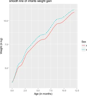
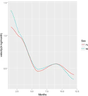
The growth of infants by weight was monotonically increasing over age (see Figures 1 and 2). Boys seem heavier than girls. The rate of weight growth declined from birth to about age of 6.8 months, then increased up to 8.8 months and finally decreased up to one year. The rates of growth behave similarly for both boys and girls. The speed of growth seems

happening at two age points at around 6.8 and 8.8 months. Thus, the rate of weight growth of the infants had shown two optimal points. This may imply that there were two inflections points of the growth curve at one at about the 6.8 and another at 8.8 months.

5.0 7.5 10.0

0.0 2.5 5.0 7.5 10.0 12.5

Age (in months)

W

e

ig

h

t

(i

n

k

g

)

Sex

Female

Male

Figure 2. Mean smooth line curve (left) and weight growth velocity curve (right) of infants weight growth.

The variation in weights as measured by coefficient of variation declined over age (see Figure 3). The variation was

the highest (12.7%) at birth and smallest (9.4%) at the end of the study (at 12 months).

Figure 3. Plot of mean weight growth in kg over time.

Analysis of the Bayesian hierarchical model

The parameters were estimated based on simulations under the Gibbs sampler algorithm. The code was written and implemented in the R package version 3.4.2.

Prior information regarding the posterior parameter estimation was used in the Bayesian approach that takes the non-informative priors. The Gibbs sampler algorithms have

been run with the non-informative priors. Figures 4 – 6 display simulations from the posterior distributions of the parameters with 20,000 realizations for each. All the series were converged faster. From the simulated realizations of each parameter, 1000 samples were taken after burn-in of 10000 with random jumps of ten simulated values.

0.5 1.0 1.5

2.5 5.0 7.5 10.0 12.5

Months

v

e

lo

c

it

y

(i

n

k

g

/m

o

n

th

)

Sex

Female

Figure 4. Time series plots of realizations of the posterior parameters for 20, 000 iterations.

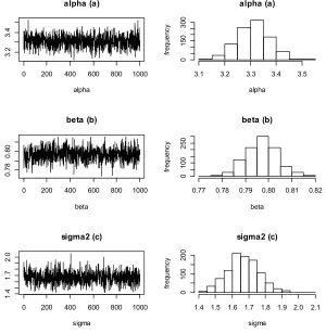
Posterior samples are displayed in Figures 5 and 6. The respective histograms plotted represent estimated posterior distributions of the parameters α, β, σ , \_], \_^. They are solutions to the problem under study.

Figure 5. Time series plots and histograms of randomly sampled posterior parameters (B, C, { ) after burn-in.

0 5000 10000 15000 20000

3

.1

3

.3

3

.5

alpha (a)

0 5000 10000 15000 20000

0

.7

7

0

.8

0

beta (b)

0 5000 10000 15000 20000

2

4

6

8

sigma2 (c)

0 5000 10000 15000 20000

0

1

0

0

2

0

0

tau.alpha (d)

0 5000 10000 15000 20000

1

0

0

2

0

0

3

0

0

tau.beta (e)

0 200 400 600 800 1000

3

.2

3

.4

alpha (a)

alpha

alpha (a)

alpha

fr

e

q

u

e

n

c

y

3.1 3.2 3.3 3.4 3.5

0

1

5

0

3

0

0

0 200 400 600 800 1000

0

.7

8

0

.8

0

beta (b)

beta

beta (b)

beta

fr

e

q

u

e

n

c

y

0.77 0.78 0.79 0.80 0.81 0.82

0

1

0

0

2

5

0

0 200 400 600 800 1000

1

.4

1

.7

2

.0

sigma2 (c)

sigma

sigma2 (c)

sigma

fr

e

q

u

e

n

c

y

1.4 1.5 1.6 1.7 1.8 1.9 2.0 2.1

0

1

0

0

2

0

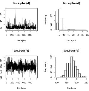
Figure 6. Time series plot and histogram of randomly sampled posterior precision parameters (\_],\_^), after burn-in.

Summary of the estimations are given in Table 2. Reliable estimates were obtained. The estimate of alpha (intercept representing birth weight) was around 3.31kg with standard deviation of 0.062 kg. The estimated of beta (slope representing rate of growth over time) was about 0.797kg with standard deviation of 0.007kg. Weight may increase by 0.797kg for one month increase in age, on average. These findings are consistent with those of [1] who reported mean birth weight of 3.25 kg for boys and 3.12 kg for girls.

The estimate of population variance was about 1.67 kg2 with standard variance of 0.096 kg2. The precision for the slope parameter estimator was quite higher than that of the intercept.

Table 2. Posterior parameters estimates based on the simulated samples.

Paramete rs

Estimated values 95% confidence intervals Mean Variance Upper limit Lower limit

α 3.310 0.00380 3.18 3.42

β 0.797 0.00005 0.78 0.81

2

σ 1.667 0.00930 1.47 1.87

α

τ 6.1 7.2 3.1 12.3

β

τ 176.5 476.4 136.2 220.8

4. Discussion

This study used hierarchical and dynamic linear growth model in analyzing the weight data of infants using Bayesian methods. Growth data of 126 infants, from birth to one year

old were obtained from Adare General Hospital in Hawassa City Administration.

The posterior distribution was obtained as a solution to the defined problem studied. Birth weight was found to have normal distribution with mean 3.31kg with standard deviation of 0.062 kg. Slope of the growth over time also had normal distribution with about 0.797 kg with standard deviation of 0.007 kg. Weight might increase by 0.797 kg for one month increased in age. The rate of growth of the infants has got two optimal points and hence two inflections points were observed at about the 6.8 and 8.8 months.

The point estimates of mean and standard deviation of the birth weight of the infants were consistent with different literature. For example, mean birth weight of newborn babies reported by [23] from a study at the Teaching Referral Hospital of Gonder, Ethiopia, was around 3.0 kg. Other study [24] reported the mean birth weight for term babies was 3.3 ±0.5 kg. [1], reported that mean birth weight was 3.25±0.51 kg for boys and 3.115±0.48 kg for girls. Other study (see www.webmd.boots.com/normal-baby-sizeat-birth) also reported that normal weight of a baby who reaches full term between 37 and 40 weeks was 3.5kg on average.

The Bayesian hierarchical and dynamic linear model is found to be convenient in explaining the weight growth of infants. For instance, [21] used hierarchical and dynamic simple linear regression model to describe the weight gain patterns of 68 pregnant women in Brazil.

0 200 400 600 800

5

1

5

2

5

tau.alpha (d)

tau.alpha

tau.alpha (d)

tau.alpha

fr

e

q

u

e

n

c

y

5 10 15 20 25 30 35

0

1

0

0

3

0

0

0 200 400 600 800

1

0

0

1

4

0

1

8

0

2

2

0

tau.beta (e)

tau.beta

tau.beta (d)

tau.beta

fr

e

q

u

e

n

c

y

100 150 200 250

0

5

0

1

0

0

2

0

5. Conclusions

The main objective of this study was to model the biological growth of infants by weight during the first year of their lives using the Bayesian hierarchical and dynamic linear regression model. There has been a sample of 126 infants under follow-up from birth to 12 months old at Adare General Hospital, Hawassa Ethiopia. A total of 756 weight measurement observations were collected from the following-up of the infants during the one year period. The Bayesian hierarchical and dynamic linear regression model isexplored their growth incorporating individual and population level variations over observed time.

The mean weight growth of the infants was found to be linearly increasing over one year period. However, the variation in weights as measured by coefficient of variation declines over age. The speed of growth declines up to about 6.8 months, and then increases up to 8.8 months, then declines up to endof the year. Thus the rate of growth has two optimums and hence weight growth has two inflections points at about the 6.8 and 8.8 months.

The mean birth weight was found to have normal distribution with mean 3.31kg and standard deviation 0.062 kg, while the weight at birth (slope) had normal distribution with mean 0.797 kg and standard deviation 0.007kg. The Bayesian hierarchical and dynamic linear model can be used to capture dynamic weight gain pattern it could be convenient method in explaining growth of the infants considered.

This study considers only infants born and visiting one hospital and residing in one city. The results from this study may not be generalized to larger population. Thus, further research is recommended to larger datasets for more inferences.

Ethical Considerations

Ethics approval was obtained from the Adare General Hospital ethical committee. Informed consent was obtained from the mothers of the infants considered. All parents provided written informed consent prior to data collection. Research approval was obtained the Hawassa University.

Acknowledgements

Authors would like to appreciate Hawassa cohort study, infants’ mothers, data collector nurses (Abinet and Meskele) and medical director of the Adare General Hospital. Their kindness and willingness to corporate with and support the study was highly encouraging. Many thanks to you for the friendship, encouragement and the fun we shared.

References

[1] Spyrides, M. H. C., Struchiner, CJ, Tereza, M., Barbosa, S. and Kac G., (2008). Effect of Predominant Breastfeeding Duration on Infant Growth: A Prospective Study using Nonlinear Mixed Effect Models. J Pediatr (Rio J), 84(3) pp. 237-243.

[2] Baker J., (2013). New Analytic Approaches in Auxology, Pediatric Research,74(1) pp. 2-4.

[3] Driver C. C. and Voelkle M. C., (2016). Hierarchical Bayesian Continuous Time Dynamic Modeling; Unpublished Draft manuscript, pp. 1-19.

[4] Oravecz Z. and Muth C., (2017). Fitting Growth Curve Models in the Bayesian Framework. Springer link, pp. 1-21. [5] Chirwa E. D., Griffiths P. L., Maleta K., Norris S. A.,

Cameron N., (2014). Multilevel Modeling of Longit udinal Child Growth Data from Birth to Twenty Cohorts: A Comparison of Growth Models. Annals of Human Biology. Journal of the Society for the Study of Human Biology, 41(2) pp. 168-179.

[6] Grimm K. J., Ram N., and Hamagami F., (2011): Nonlinear Growth Curves in Developmental Research. Child Development, 82 (5) pp. 1357–1371.

[7] Johnson W., Balakrishna N., and Griffiths P. L., (2013). Modeling Physical Growth using Mixed Effects Models. Am J PhysAnthropol, 150 (1): 58–67.

[8] Stirnemann J. J, Samson A., and Thalabard J. C., (2011). Individual Predictions based on Nonlinear Mixed Modeling: Application to Prenatal Twin Growth. Statistics in Medicine, 00 pp. 1–15.

[9] Wang J., Luo S., and Li L., (2016). Dynamic Prediction for Multiple Repeated Measures and Event Time Data: An Application to Parkinson’s Disease. Cornell University Library.

[10] Gliozzi A. S., Guiot C., Delsanto P. P. and Iordach D. A., (2012). A Novel Approach to the Analysis of Human Growth. Theoretical Biology and Medical Modelling, 9 pp 1-17.

[11] Richard S. A., Benjamin J. J., and McCormick C. W., (2014). Modeling Environmental Influences on Child Growth in the MALED Cohort Study: Opportunities and Challenges. Clinical Infectious Diseases, 59 (4) pp. 255–60.

[12] Cameron N., (2012): Human Growth Curve Canalization, and Catch-up Growth. In: Cameron, N. Editor. Human Growth and Development. pp. 1-24.

[13] Brown W., and Leckie G., (2014). Modelling Longitudinal Data using the Stat-JR package. National Center for Research Methods (NCRM). Centre for Multilevel Modelling, University of Bristol.

[14] Tenan S., (2012). Hierarchical Bayesian Modeling and Application in Animal Population Ecology. Unpublished PhD Thesis. University of Pavia.

[15] Petris, G., Petrone, S., Compagnoli, P. (2007). Dynamic Linear Models with R. Monography. Springer

[16] Huang Y., Liu D., and Wu H., (2006). Hierarchical Bayesian Methods for Estimation of Parameter in the Longitudinal HIV Dynamic Systems. Biometrics, 62 (2) pp. 413-423.

[17] Gelman A., Carlin J. B., Stern H. S., and Rubin D. B., (2013): Bayesian Data Analysis (3rded). Boca Raton, F L.: Chapman & Hall/CRC.

[19] McElreath R.., (2016). Statistical Rethinking: A Bayesian Course with Examples in R and Stan. A Chapman & Hall book Volume 122 of Chapman & Hall/CRC texts in statistical science series Volume 122 of Texts in statistical science, CRC Press/Taylor & Francis Group.

[20] Gamerman D., and Loopes H. F., (2006). Markov Chain Monte Carlo Stochastic Simulation for Bayesian Inference (2ndEdition). Chapman and Hall/CRC.

[21] Souza A. P., (1999). Approximate Methods in Bayesian Dynamic Hierarchical Models. Unpublished PhD Thesis. [22] Carlin B. C. and Louis T. A., (1996). Bayes and Empirical

Bayes Methods for Data Analysis. Chapman& Hall, London.

[23] Teshome D., Telahun T., Solomon D., and Abdulhamid I., (2006). A Study on Birth Weight in a Teaching Referral Hospital, Gonder, Ethiopia. Cent Afr J Med, 52(1-2) pp. 8-11. [24] Bhutta Z. A., Das J. K., Rizvi A., Gaffey M. F., Walker N.,