Optimized Cutting Plane Algorithm for
Large-Scale Risk Minimization
∗Vojtˇech Franc [email protected]
Center for Machine Perception Department of Cybernetics Faculty of Electrical Engineering Czech Technical University in Prague Technicka 2, 166 27 Praha 6,
Czech Republic
S¨oren Sonnenburg [email protected]
Friedrich Miescher Laboratory Max Planck Society
Spemannstr. 39
72076 T¨ubingen, Germany
Editor: Michele Sebag
Abstract
We have developed an optimized cutting plane algorithm (OCA) for solving large-scale risk mini-mization problems. We prove that the number of iterations OCA requires to converge to aεprecise solution is approximately linear in the sample size. We also derive OCAS, an OCA-based linear bi-nary Support Vector Machine (SVM) solver, and OCAM, a linear multi-class SVM solver. In an ex-tensive empirical evaluation we show that OCAS outperforms current state-of-the-art SVM solvers like SVMlight, SVMperfand BMRM, achieving speedup factor more than 1,200 over SVMlighton some data sets and speedup factor of 29 over SVMperf, while obtaining the same precise sup-port vector solution. OCAS, even in the early optimization steps, often shows faster convergence than the currently prevailing approximative methods in this domain, SGD and Pegasos. In addi-tion, our proposed linear multi-class SVM solver, OCAM, achieves speedups of factor of up to 10 compared to SVMmulti−class. Finally, we use OCAS and OCAM in two real-world applications, the problem of human acceptor splice site detection and malware detection. Effectively paral-lelizing OCAS, we achieve state-of-the-art results on an acceptor splice site recognition problem only by being able to learn from all the available 50 million examples in a 12-million-dimensional feature space. Source code, data sets and scripts to reproduce the experiments are available at http://cmp.felk.cvut.cz/˜xfrancv/ocas/html/.
Keywords: risk minimization, linear support vector machine, multi-class classification, binary classification, large-scale learning, parallelization
1. Introduction
Many applications in, for example, bioinformatics, IT-security and text classification come with huge numbers (e.g., millions) of data points, which are indeed necessary to obtain
art results. They, therefore, require extremely efficient computational methods capable of dealing with ever growing data sizes. A wide range of machine learning methods can be described as the unconstrained regularized risk minimization problem
w∗=argmin
w∈ℜn
F(w):=1 2kwk
2+CR(w), (1)
where w∈ℜndenotes the parameter vector to be learned,1
2kwk2is a quadratic regularization term,
C>0 is a fixed regularization constant and R : ℜn →ℜ is a non-negative convex risk function approximating the empirical risk (e.g., training error).
Special cases of problem (1) are, for example, support vector classification and regression (e.g., Cortes and Vapnik, 1995; Cristianini and Shawe-Taylor, 2000), logistic regression (Collins et al., 2000), maximal margin structured output classification (Tsochantaridis et al., 2005), SVM for multi-variate performance measures (Joachims, 2005), novelty detection (Sch¨olkopf et al., 1999), learning Gaussian processes (Williams, 1998) and many others.
Problem (1) has usually been solved in its dual formulation, which typically only uses the com-putation of dot products between examples. This enables the use of kernels that implicitly compute the dot product between examples in a Reproducing Kernel Hilbert Space (RKHS) (Sch¨olkopf and Smola, 2002). On the one hand, solving the dual formulation is efficient when dealing with high-dimensional data. On the other hand, efficient and accurate solvers for optimizing the kernelized dual formulation for large sample sizes do not exist.
Recently, focus has shifted towards methods optimizing problem (1) directly in the primal. Using the primal formulation is efficient when the number of examples is very large and the di-mensionality of the input data is moderate or the inputs are sparse. This is typical in applications like text document analysis and bioinformatics, where the inputs are strings embedded into a sparse high-dimensional feature space, for example, by using the bag-of-words representation. A way to exploit the primal formulation for learning in the RKHS is based on decomposing the kernel matrix and thus effectively linearizing the problem (Sch¨olkopf and Smola, 2002).
Due to its importance, the literature contains a plethora of specialized solvers dedicated to particular risk functions R(w) of problem (1). Binary SVM solvers employing the hinge risk R(w) = 1
m∑ m
i=1max{0,1−yihw,xii}especially have been studied extensively (e.g., Joachims, 1999; Zanni et al., 2006; Chang and Lin, 2001; Sindhwani and Keerthi, 2007; Chapelle, 2007; Lin et al., 2007). Recently, Teo et al. (2007) proposed the Bundle Method for Risk Minimization (BMRM), which is a general approach for solving problem (1). BMRM is not only a general but also a highly modular solver that only requires two specialized procedures, one to evaluate the risk R(w)and one to compute its subgradient. BMRM is based on iterative approximation of the risk term by cutting planes. It solves a reduced problem obtained by substituting the cutting plane approximation of the risk into the original problem (1). Teo et al. (2007) compared BMRM with specialized solvers for SVM classification, SV regression and ranking, and reported promising results. However, we will show that the implementation of the cutting plane algorithm (CPA) used in BMRM can be dras-tically sped up making it efficient even for large-scale SVM binary and multi-class classification problems.
(master) problem (1). Second, we introduce a new cutting plane selection strategy that reduces the number of cutting planes required to achieve the prescribed precision and thus significantly speeds up convergence. An efficient line-search procedure for the optimization of (1) is the only additional requirement of OCA compared to the standard CPA (or BMRM).
While our proposed method (OCA) is applicable to a wide range of risk terms R, we will—due to their importance—discuss in more detail two special cases: learning of the binary (two-class) and multi-class SVM classifiers. We show that the line-search procedure required by OCA can be solved exactly for both the binary and multi-class SVM problems in O(m log m) and O(m·Y2+ m·Y log(m·Y)) time, respectively, where m is the number of examples and Y is the number of classes. We abbreviate OCA for binary SVM classifiers with OCAS and the multi-class version with OCAM.
We perform an extensive experimental evaluation of the proposed methods, OCAS and OCAM, on several problems comparing them with the current state of the art. In particular, we would like to highlight the following experiments and results:
• We compare OCAS with the state-of-the-art solvers for binary SVM classification on pre-viously published data sets. We show that OCAS significantly outperforms the competing approaches achieving speedups factors of more than 1,200.
• We evaluate OCAS using the large-scale learning challenge data sets and evaluation protocols described in Sonnenburg et al. (2009). Although OCAS is an implementation of a general method for risk minimization (1), it is shown to be competitive with dedicated binary SVM solvers, which ultimately won the large-scale learning challenge.
• We demonstrate that OCAS can be sped up by efficiently parallelizing its core subproblems.
• We compare OCAM with the state-of-the-art implementation of the CPA-based solver for training multi-class SVM classifiers. We show that OCAM achieves speedups of an order of magnitude.
• We show that OCAS and OCAM achieve state-of-the-art recognition performance for two real-world applications. In the first application, we attack a splice site detection problem from bioinformatics. In the second, we address the problem of learning a malware behavioral classifier used in computer security systems.
The OCAS solver for training the binary SVM classification was published in our previous paper (Franc and Sonnenburg, 2008a). This paper extends the previous work in several ways. First, we formulate OCA for optimization of the general risk minimization problem (1). Second, we give an improved convergence proof for the general OCA (in Franc and Sonnenburg 2008a the upper bound on the number of iterations as a function of precision ε scales with
O
(1ε2), while in this
paper the bound is improved to
O
(1ε)). Third, we derive a new instance of OCA for training the
multi-class SVM classifiers. Fourth, the experiments are extended by (i) including the comparison on the challenge data sets and using the challenge protocol, (ii) performing experiments on multi-class multi-classification problems and (iii) solving two real-world applications from bioinformatics and computer security.
of CPA and propose a new optimized cutting plane algorithm (OCA) to drastically reduce training times. We then develop OCA for two special cases linear binary SVMs (OCAS, see Section 3.1) and linear multiclass SVMs (OCAM, see Section 3.2). In Section 4, we empirically show that using OCA, training times can be drastically reduced on a wide range of large-scale data sets including the challenge data sets. Finally, we attack two real-world applications. First, in Section 5.1, we apply OCAS to a human acceptor splice site recognition problem achieving state-of-the art results by training on all available sequences—a data set of 50 million examples (itself about 7GB in size) using a 12 million dimensional feature space. Second, in Section 5.2, we apply OCAM to learn a behavioral malware classifier and achieve a speedup of factor of 20 compared to the previous approach and a speedup of factor of 10 compared to the state-of-the-art implementation of the CPA. Section 6 concludes the paper.
2. Cutting Plane Algorithm
In CPA terminology, the original problem (1) is called the master problem. Using the approach of Teo et al. (2007), one may define a reduced problem of (1) which reads
wt=argmin
w
Ft(w):=
h1
2kwk
2+CR
t(w)
i
. (2)
(2) is obtained from master problem (1) by substituting a piece-wise linear approximation Rtfor the risk R. Note that only the risk term R is approximated while the regularization term 12kwk2remains unchanged. The idea is that in practise one usually needs only a small number of linear terms in the piece-wise linear approximation Rt to adequately approximate the risk R around the optimum
w∗. Moreover, it was shown in Teo et al. (2007) that the number of linear terms needed to achieve arbitrary precise approximation does not depend on the number of examples.
We now derive the approximation to R. Since the risk term R is a convex function, it can be approximated at any point w′by a linear under estimator
R(w)≥R(w′) +ha′,w−w′i, ∀w∈ℜn, (3)
where a′∈∂R(w′)is any subgradient of R at the point w′. We will use a shortcut b′=R(w′)−ha′,w′i to abbreviate (3) as R(w)≥ ha′,wi+b′. In CPA terminology, ha′,wi+b′ =0 is called a cutting plane.
To approximate the risk R better than by using a single cutting plane, we can compute a collec-tion of cutting planes{hai,wi+bi=0|i=1, . . . ,t}at t distinct points{w1, . . . ,wt}and take their point-wise maximum
Rt(w) =max
0, max
i=1,...,t hai,wi+bi . (4)
The zero cutting plane is added to the maximization as the risk R is assumed to be non-negative. The subscriptt denotes the number of cutting planes used in the approximation Rt. It follows directly from (3) that the approximation Rt is exact at the points{w1, . . . ,wt}and that Rt lower bounds R, that is, that R(w)≥Rt(w),∀w∈ℜnholds. In turn, the objective function Ft of the reduced problem lower bounds the objective F of the master problem.
Having readily computed Rt,we may now use it in the reduced problem (2). Substituting (4) with (2), the reduced problem can be expressed as a linearly constrained quadratic problem
(wt,ξt):= argmin
w∈ℜn,ξ∈ℜ
h1
2kwk
subject to
ξ≥0, ξ≥ hai,wi+bi, i=1, . . . ,t.
The number of constraints in (5) equals the number of cutting planes t which can be drastically lower than the number of constraints in the master problem (1) when expressed as a constrained QP task. As the number of cutting planes is typically much smaller than the data dimensionality n, it is convenient to solve the reduced problem (5) by optimizing its dual formulation, which reads
αt :=argmax α∈At
Dt(α):=
h t
∑
i=1αibi− 1 2
t
∑
i=1aiαi
2i
, (6)
where
A
t is a convex feasible set containing all vectorsα∈ℜt satisfying t∑
i=1αi≤C, αi≥0,i=1, . . . ,t.
The dual formulation contains only t variables bound by t+1 constraints of simple form. Thus task (6) can be efficiently optimized by standard QP solvers. Having (6) solved, the primal solution can be computed as
wt =− t
∑
i=1ai[αt]i, and ξt= max
i=1,...,t(hwt,aii+bi).
Solving the reduced problem is beneficial if we can effectively select a small number of cutting planes such that the solution of the reduced problem is sufficiently close to the master problem. CPA selects the cutting planes using a simple strategy described by Algorithm 1.
Algorithm 1 Cutting Plane Algorithm (CPA)
1: t :=0. 2: repeat
3: Compute wt by solving the reduced problem (5).
4: Add a new cutting plane to approximate the risk R at the current solution wt, that is, compute
at+1∈∂R(wt)and bt+1:=R(wt)− hat+1,wti. 5: t :=t+1
6: until a stopping condition is satisfied.
The algorithm is very general. To use it for a particular problem one only needs to supply a formula to compute the cutting plane as required in Step 4, that is, formulas for computing the subgradient a∈∂R(w)and the objective value R(w)at given point w.
It is natural to stop the algorithm when
F(wt)−Ft(wt)≤ε (7)
holds. Because Ft(wt) is the lower bound of the optimal value, F(w∗), it follows that a solution
wt satisfying (7) also guarantees F(wt)−F(w∗)≤ε, that is, the objective value differs from the optimal one byε at most. An alternative stopping condition advocated in Joachims (2006) stops the algorithm when R(wt)−Rt(wt)≤εˆ. It can be seen that the two stopping conditions become equivalent if we setε=Cˆε. Hence we will consider only the former stopping condition (7).
Theorem 1 (Teo et al., 2007) Assume thatk∂R(w)k ≤G for all w∈
W
, whereW
is some domain of interest containing all wt′ for t′≤t. In this case, for anyε>0 and C>0, Algorithm 1 satisfies the stopping condition (7) after at mostlog2 F(0) 4C2G2+
8C2G2
ε −2
iterations.
3. Optimized Cutting Plane Algorithm (OCA)
We first point out a source of inefficiency in CPA and then propose a new method to alleviate the problem.
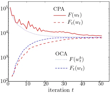
CPA selects a new cutting plane such that the reduced problem objective function Ft(wt) mono-tonically increases w.r.t. the number of iterations t. However, there is no such guarantee for the master problem objective F(wt). Even though it will ultimately converge arbitrarily close to the minimum F(w∗),its value can heavily fluctuate between iterations (Figure 1). The reason for these
0 10 20 30 40 50
102
103
104
105
CPA
OCA F(wb
t)
Ft(wt)
Ft(wt)
F(wt)
iterationt
Figure 1: Convergence behavior of the standard CPA vs. the proposed OCA.
fluctuations is that at each iteration t, CPA selects the cutting plane that perfectly approximates the master objective F at the current solution wt. However, there is no guarantee that such a cutting plane will be an active constraint in the vicinity of the optimum w∗, nor must the new solution wt+1
of the reduced problem improve the master objective. In fact, it often occurs that F(wt+1)>F(wt). As a result, a lot of the selected cutting planes do not contribute to the approximation of the master objective around the optimum which, in turn, increases the number of iterations.
Change 1 We maintain the best-so-far best solution wbt obtained during the first t iterations, that is, F(wb1), . . . ,F(wbt)forms a monotonically decreasing sequence.
Change 2 The new best-so-far solution wb
t is found by searching along a line starting at the previous solution wtb−1and crossing the reduced problem’s solution wt, that is,
wtb=min k≥0F(w
b
t−1(1−k) +wtk). (8)
Change 3 The new cutting plane is computed to approximate the master objective F at a point wc
t which lies in a vicinity of the best-so-far solution wtb. In particular, the point wct is computed as
wtc=wbt(1−µ) +wtµ, (9) where µ∈(0,1]is a prescribed parameter. Having the point wct, the new cutting plane is given by at+1∈∂R(wct)and bt+1=R(wct)− hat+1,wcti.
Algorithm 2 describes the proposed OCA. Figure 1 shows the impact of the proposed changes to the convergence. OCA generates a monotonically decreasing sequence of master objective values and a monotonically and strictly increasing sequence of reduced objective values, that is,
F(wb1)≥. . .≥F(wbt), and F1(w1)< . . . <Ft(wt).
Note that for CPA only the latter is satisfied. Similar to CPA, a natural stopping condition for OCA reads
F(wtb)−Ft(wt)≤ε, (10)
where ε>0 is a prescribed precision parameter. Satisfying the condition (10) guarantees that F(wtb)−F(w∗)≤εholds.
Algorithm 2 Optimized Cutting Plane Algorithm (OCA)
1: Set t :=0 and wb0:=0.
2: repeat
3: Compute wt by solving the reduced problem (5).
4: Compute a new best-so-far solution wbt using the line-search (8).
5: Add a new cutting plane: compute at+1∈∂R(wct)and bt+1:=R(wct)− hat+1,wtciwhere wct is given by (9).
6: t :=t+1
7: until a stopping condition is satisfied
Theorem 2 Assume thatk∂R(w)k ≤G for all w∈
W
, whereW
is some domain of interest con-taining all wt′ for t′≤t. In this case, for anyε>0, C>0 and µ∈(0,1], Algorithm 2 satisfies the stopping condition (10) after at mostlog2 F(0) 4C2G2+
8C2G2
ε −2
Theorem 2 is proven in Appendix A. Finally, there are two relevant remarks regarding Theo-rem 2:
Remark 1 Although Theorem 2 holds for any µ from the interval (0,1] its particular value has impact on the convergence speed in practice. We found experimentally (see Section 4.1) that µ=0.1 works consistently well throughout experiments.
Remark 2 Note that the bound on the maximal number of iterations of OCA given in Theorem 2
coincides with the bound for CPA in Theorem 1. Despite the same theoretical bounds, in practice OCA converges significantly faster compared to CPA, achieving speedups of more than one order of magnitude as will be demonstrated in the experiments (Section 4). In the convergence analysis (see Appendix A) we give an intuitive explanation of why OCA converges faster than CPA.
In the following subsections we will use the OCA Algorithm 2 to develop efficient binary linear and multi-class SVM solvers. To this end, we develop fast methods to solve the problem-dependent subtasks, the line-search step (step 4 in Algorithm 2) and the addition of a new cutting plane (step 5 in Algorithm 2).
3.1 Training Linear Binary SVM Classifiers
Given an example set{(x1,y1), . . . ,(xm,ym)} ∈(ℜn× {−1,+1})m, the goal is to find a parameter vector w∈ℜnof the liner classification rule h(x) =sgnhw,xi. The parameter vector w is obtained by minimizing
F(w):=1 2kwk
2+C
m m
∑
i=1max{0,1−yihw,xii}, (11)
which is a special instance of the regularized risk minimization problem (1) with the risk
R(w):= 1 m
m
∑
i=1max{0,1−yihw,xii}. (12)
It can be seen that (12) is a convex piece-wise linear approximation of the training errorm1∑mi=1[[h(xi)6= yi]].
To use the OCA Algorithm 2 for solving (12), we need the problem-dependent steps 4 and 5. First, we need to supply a procedure performing the line-search (8) as required in Step 4. Sec-tion 3.1.1 describes an efficient algorithm solving the line-search exactly in
O
(m log m)time. Sec-ond, Step 5 requires a formula for computing a subgradient a∈∂R(w)of the risk (12) which readsa=−1 m
m
∑
i=1πiyixi, πi=
1 if yihw,xii ≤1, 0 if yihw,xii>1.
3.1.1 LINE-SEARCHFORLINEARBINARYSVM CLASSIFIERS
The line-search (8) requires minimization of a univariate convex function
F(wtb−1(1−k) +wtk) = 1 2kw
b
t−1(1−k) +wtkk2+CR(wbt−1(1−k) +wtk), (13) with R defined by (12). Note that the line-search very much resembles the master problem (1) with one-dimensional data. We show that the line-search can be solved exactly in
O
(m log m)time.We abbreviate F(wbt−1(1−k) +wtk)by f(k)which is defined as
f(k):= f0(k) +
m
∑
i=1fi(k) =
1 2k
2A
0+kB0+C0+
m
∑
i=1max{0,kBi+Ci},
where
A0 = kwbt−1−wtk2
B0 = hwtb−1,wt−wbt−1i, Bi = Cmyihxi,wbt−1−wti,i=1, . . . ,m, C0 =
1 2kw
b
t−1k2, Ci = Cm(1−yihxi,wbt−1i),i=1, . . . ,m.
(14)
Hence the line-search (8) involves solving k∗=argmink≥0f(k)and computing wb
t =wbt−1(1−k∗) + wtk∗. Since f(k)is a convex function, its unconstrained minimum is attained at the point k∗, at which the sub-differential∂f(k)contains zero, that is, 0∈∂f(k∗)holds. The subdifferential of f reads
∂f(k) =kA0+B0+
m
∑
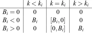
i=1∂fi(k), where ∂fi(k) =
0 if kBi+Ci<0, Bi if kBi+Ci>0,
[0,Bi] if kBi+Ci=0.
Note that the subdifferential is not a function because there exist k’s for which∂f(k)is an interval. The first term of the subdifferential∂f(k)is an ascending linear function kA0+B0since A0must be
greater than zero. Note that A0=kwbt−1−wtk2equals 0 only if the algorithm has converged to the optimum w∗, but in this case the line-search is not invoked. The term∂fi(k)appearing in the sum is
k<ki k=ki k>ki
Bi=0 0 0 0
Bi<0 Bi [Bi,0] 0 Bi>0 0 [0,Bi] Bi
Table 1: The value of∂fi(k)with respect to k.
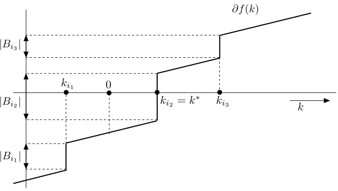
either constantly zero, if Bi=0, or it is a step-like jump whose value changes at the point ki=−CBii. In particular, the value of∂fi(k)w.r.t. k is summarized in Table 1. Hence the subdifferential∂f(k) is a monotonically increasing function as is illustrated in Figure 2. To solve k∗=argmink≥0f(k)we proceed as follows:
1. We compute the maximal value of the subdifferential∂f(k)at point 0:
max(∂f(0)) =B0+
m
∑
i=12. If max(∂f(0))is strictly greater than zero, we know that the unconstrained minimum
argmink f(k) is attained at a point less than or equal to 0. Thus, the constrained minimum k∗=argmink≥0f(k), that is, the result of the line-search, is attained at the point k∗=0. 3. If max(∂f(0))is less than zero, then the optimum k∗=argmink≥0f(k) corresponds to the
unconstrained optimum argmink f(k). To get k∗we need to find an intersection between the graph of∂f(k)and the x-axis. This can be done efficiently by sorting points K={ki|ki> 0,i=1, . . . ,m} and checking the condition 0∈∂f(k) for k∈K and for k in the intervals which split the domain(0,∞)in the points K. These computations are dominated by sorting the numbers K, which takes
O
(|K|log|K|)time.Computing the parameters (14) of the function f(k)requires
O
(mn)time, where m is the number of examples and n is the number of features. Having the parameters computed, the worst-case time complexities of the steps 1, 2 and 3 areO
(m),O
(1)andO
(m log m), respectively.3.1.2 PARALLELIZATION
Apart from solving the reduced problem (2), all subtasks of OCAS can be efficiently parallelized:
Output computation. This involves computation of the dot productshwt,xii for all i=1, . . . ,m, which requires
O
(s)time, where s equals the number of all non-zero elements in the training examples. Distributing the computation equally to p processors reduces the effort toO
(sp). Note that the remaining products with data required by OCAS, that is,hwbt,xiiandhwct,xii, can be computed fromhwt,xiiin time
O
(m).ki1
ki3
ki2 =k
∗ |Bi2|
|Bi1|
|Bi3|
0
k
∂f(k)
Figure 2: Graph depicting the subdifferential∂f(k)of the objective function f(k). The line-search requires computing k∗=mink≥0f(k) which is equivalent to finding the intersection k∗
Line-search. The dominant part is sorting|K|numbers which can be done in
O
(|K|log|K|)time. A speedup can be achieved by parallelizing the sorting function by using p processors, reducing time complexity toO
|K|logp|K|. Note that our implementation of OCAS uses quicksort, whose worst-case time complexity is
O
(|K|2),although its expected run-time isO
(|K|log|K|).Cutting plane computation. The dominant part requires the sum −m1∑mi=1πiyixi, which can be done in
O
(sπ) time, where sπ=|{i|πi =6 0, ∀i=1, . . . ,m}| is the number of non-zero πi.Using p processors results in a time complexity of
O
(sπ p).It is worth mentioning that OCAS usually requires a small number of iterations (usually less than 100 and almost always less than 1000). Hence, solving the reduced problem, which cannot be parallelized, is not the bottleneck, especially when the number of examples m is large.
3.2 Training General Linear Multi-Class SVM Classifiers
So far we have assumed that (i) the ultimate goal is to minimize the probability of misclassification, (ii) the input observations x are vectors from ℜn and (iii) the label y can attain only two values {−1,+1}. In this section, we will consider the regularized risk minimization framework applied to the learning of a general linear classifier (Tsochantaridis et al., 2005).
We assume that the input observation x is from an arbitrary set
X
and the label y can have values fromY
={1, . . . ,Y}. In addition, letδ:Y
×Y
→ℜbe an arbitrary loss function which satisfiesδ(y,y) =0,∀y∈Y
, andδ(y,y′)>0,∀(y,y′)∈Y
×Y
, y6=y′. We consider the multi-class classification rule h :X
→Y
defined ash(x; w) =argmax y∈Y
hw,Ψ(x,y)i,
where w∈ℜd is a parameter vector andΨ:
X
×Y
→ℜdis an arbitrary map from the input-output space to the parameter space. Given example set{(x1,y1), . . . ,(xm,ym)} ∈(X
×Y
)m, learning the parameter vector w using the regularized risk minimization framework requires solving problem (1) with the empirical risk Remp(h(·; w)) = m1∑mi=1δ(h(xi),yi). Tsochantaridis et al. (2005) propose two convex piece-wise linear upper bounds on risk Remp(h(·; w)). The first one, called the marginre-scaling approach, defines the proxy risk as
R(w):= 1 m
m
∑
i=1max
y∈Y δ(y,yi) +hΨ(xi,y)−Ψ(xi,yi),wi
. (15)
The second one, called the slack re-scaling approach, defines the proxy risk as
R(w):= 1 m
m
∑
i=1max
y∈Y δ(y,yi) 1+hΨ(xi,y)−Ψ(xi,yi),wi
. (16)
To use the OCA Algorithm 2 for the regularized minimization of (15), we need, first, to derive a procedure performing the line-search (8) required in Step 4 and, second, to derive a formula for the computation of the subgradient of the risk R as required in Step 5. Section 3.2.1 describes an efficient algorithm solving the line-search exactly in
O
(m·Y2+m·Y log(m·Y))time. The formula for computing the subgradient a∈∂R(w)of the risk (15) readsa= 1 m
m
∑
i=1Ψ(xi,yˆi)−Ψ(xi,yi)
,
where
ˆ
yi=argmax y∈Y
δ(yi,y) +hΨ(xi,y)−Ψ(xi,yi),wi
.
We call the resulting method the optimized cutting plane algorithm for multi-class SVM (OCAM). Finally, note that the subtasks of OCAM can be parallelized in a fashion similar to the binary case (see Section 3.1.2).
3.2.1 LINE-SEARCHFORGENERALMULTI-CLASS LINEARSVM CLASSIFIERS
In this section, we derive an efficient algorithm to solve the line-search (8) for the margin re-scaling risk (15). The algorithm is a generalization of the line-search for the binary SVM described in Section 3.1.1. Since the core idea remains the same we only briefly describe the main differences.
The goal of the line-search is to minimize a univariate function F(wbt−1(1−k) +wtk)defined by (13) with the risk R given by (15). We can abbreviate F(wtb−1(1−k) +wtk)by f(k)which reads
f(k):= f0(k) +
m
∑
i=1fi(k) =
1 2k
2A
0+kB0+C0+
m
∑
i=1max y∈Y kB
y i +C y i ,
where the constants A0, B0, C0,(Byi,C y
i),i=1, . . . ,m,y∈
Y
are computed accordingly. Similar to the binary case, the core idea is to find an explicit formula for the subdifferential ∂f(k), which, consequently, allows solving the optimality condition 0∈∂f(k). For a given fi(k), let ˆY
i(k) ={y∈Y
|kByi+Ciy=maxy′∈Y kBy′ i +C
y′ i
}be a set of indices of the linear terms which are active at the point k. Then the subdifferential of f(k)reads
∂f(k) =kA0+B0+
m
∑
i=1∂fi(k) where ∂fi(k) =co{Byi |y∈
Y
ˆi(k)}. (17)The subdifferential (17) is composed of a linear term kA0+B0and a sum of maps∂fi:ℜ→
I
, i=1, . . . ,m, whereI
is a set of all closed intervals on a real line. From the definition (17) it follows that ∂fi is a step-function (or staircase function), that is, ∂fi is composed of piece-wise linear horizontal and vertical segments. An explicit description of these linear segments is crucial for solving the optimality condition 0∈∂f(k) efficiently. Unlike the binary case, the segments cannot be computed directly from the parameters(Byi,Ciy),y∈Y
, however, they can be found by the simple algorithm described below.(B2
, C2
) k k2
i k1
i
( ˆB2
i,Cˆ
2
i) = (B
1
i, C
1
i)
fi(k) = maxy(kByi +Cik)
( ˆB3
i,Cˆ
3
i) = (B
4
i, C
4
i)
( ˆB1
i,Cˆ
1
i) = (B
3
i, C
3
i)
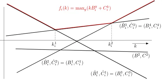
Figure 3: Figure shows an example of the function fi(k) which is defined as the point-wise maxi-mum over linear terms kByi +Ciy, y=1, . . . ,4. The parameters(Bˆz
i,Cˆiz), z=1, . . . ,3, and points kzi, z=1,2 found by Algorithm 3 are also visualized.
∂fi(k) changes. Let Z∈ {1, . . . ,Y−1}be a given integer and k1i, . . . ,kZi−1 be a strictly increasing sequence of real numbers. Then we define a system of Z open intervals{
I
1i , . . . ,
I
iZ}such thatI
1i = (−∞,ki1),
I
iZ= (kiZ−1,∞), andI
iz= (kzi−1,kzi),∀1<z<Z.It can be seen that there exist an integer Z and a sequence k1i, . . . ,kZi−1such that the map∂fi can be equivalently written as
∂fi(k) =
ˆ
Bzi if k∈
I
iz,[Bˆzi,Bˆiz+1] if k∈kzi, (18)
where{Bˆ1
i, . . . ,BˆZi}is a subset of{Bi1, . . . ,BYi}. Provided the representation (18) is known for all∂fi, i=1, . . . ,m, the line-search k∗=argmink>0f(k)can be solved exactly by finding the intersection of ∂f(k)and the x-axis, that is, solving the optimality condition 0∈∂f(k). To this end, we can use the same algorithm as in the binary case (see Section 3.1.1). The only difference is that the number of points kzi in which the subdifferential∂f(k)changes its value is higher; m·(Y−1)in the worst case. As the computations of the algorithm for solving 0∈∂f(k)are dominated by sorting the points kiz, the worst-case computational complexity is approximately
O
(m·Y log(m·Y)).Finally, we introduce Algorithm 3, which finds the required representation (18) for a given∂fi. In the description of Algorithm 3, we do not use the subscripti to simplify the notation. Figure 3 shows an example of input linear terms(Byi,Ciy), y∈
Y
defining the function fi(k)and the sorted sequence of active terms(Bˆzi,Cˆiz),z=1, . . . ,Z, and points kzi, z=1, . . . ,Z, in which the activity of the linear terms changes. At the beginning, the algorithm finds a linear term which is active in the leftmost interval(−∞,k1), that is, the line with the maximal slope. Then the algorithm computes intersections with the leftmost active linear term that was found and the remaining lines with lower slopes. The leftmost intersection identifies the next active term. This process is repeated until the rightmost active term is found. The worst-case computational complexity of Algorithm 3 is
O
(Y2).In turn, the total complexity of the line-search procedure is
O
(m·Y2+m·Y log(m·Y)), that is,Algorithm 3 Finding explicit piece-wise linear representation (18) of∂fi
Require: (By,Cy), y∈
Y
Ensure: Z,{Bˆ1, . . . ,BˆZ}, and{k1, . . . ,kZ−1}
1: y :=ˆ argmaxy∈YˆCywhere ˆ
Y
:={y|By=miny′∈YBy′}. 2: Z :=1, k :=−∞and ˆB1:=Byˆ3: while k<∞do
4:
Y
ˆ :={y|By>Byˆ}5: if ˆ
Y
is empty then6: k :=∞
7: else
8: y :=¨ argminy∈Yˆ C y−Cyˆ
By−Byˆ
9: kZ:=Cy¨−Cyˆ
By¨−Byˆ
10: Z :=Z+1 11: BˆZ:=By¨ 12: y :=ˆ y¨ 13: end if
14: end while
Note that the described algorithm is practical only if the output space
Y
is of moderate size since the complexity of the line-search grows quadratically with Y =|Y
|. For that reason, this algorithm is ineffective for structured output learning where the cardinality ofY
grows exponentially with the number of hidden states.4. Experiments
In this section we perform an extensive empirical evaluation of the proposed optimized cutting plane algorithm (OCA) applied to linear binary SVM classification (OCAS) and multi-class SVM classification (OCAM) .
In particular, we compare OCAS to various state-of-the-art SVM solvers. Since several of these solvers did not take part in the large-scale learning challenge, we perform an evaluation of SVMlight, Pegasos, GPDT, SGD, BMRM, SVMperf version 2.0 and version 2.1 on previously published medium-scale data sets (see Section 4.1.1). We show that OCAS outcompetes previous solvers gaining speedups of several orders of magnitude over some of the methods and we also analyze the speedups gained by parallelizing the various core components of OCAS.
In addition, we use the challenge data sets and follow the challenge protocol to compare OCAS with the best performing methods, which were LaRank and LibLinear (see Section 4.1.2). Finally, in section 4.2, we compare the multi-class SVM solver OCAM to the standard CPA implemented for multi-class SVM on four real-world problems using the challenge evaluation protocol.
4.1 Comparison of Linear Binary SVM
4.1.1 EVALUATION ON PREVIOUSLY USED DATASETS
We now compare current state-of-the-art SVM solvers (SGD, Pegasos, SVMlight, SVMperf , BMRM,
GPDT1), on a variety of data sets with the proposed method (OCAS), using 6 experiments measur-ing:
1. Influence of the hyper-parameter µ on the speed of convergence 2. Training time and objective for optimal C
3. Speed of convergence (time vs. objective) 4. Time to perform a full model selection 5. Effects of parallelization
6. Scalability w.r.t. data set size
To this end, we implemented OCAS and the standard CPA2in C. We use the very general com-pressed sparse column (CSC) representation to store the data. Here, each element is represented by an index and a value (each 64bit). To solve the reduced problem (2), we use our implementation of improved SMO (Fan et al., 2005). The source code of OCAS is freely available for download as part of LIBOCAS (Franc and Sonnenburg, 2008b) and as a part of the SHOGUN toolbox (Sonnenburg and R¨atsch, 2007).
All competing methods train SVM classifiers by solving the convex problem (1) either in its primal or dual formulation. Since in practice only limited precision solutions can be obtained, solvers must define an appropriate stopping condition. Based on the stopping condition, solvers can be categorized into approximative and accurate.
Approximative Solvers make use of heuristics (e.g., learning rate, number of iterations) to obtain (often crude) approximations of the optimal solution. They have a very low per-iteration cost and low total training time. Especially for large-scale problems, they are claimed to be sufficiently precise while delivering the best performance vs. training time trade-off (Bottou and Bousquet, 2007), which may be attributed to the robust nature of large-margin SVM solutions. However, while they are fast in the beginning they often fail to achieve a precise solution. Among the most efficient solvers to-date are Pegasos (Shwartz et al., 2007) and SGD (Bottou and Bousquet, 2007), both of which are based on stochastic (sub-)gradient descent.
Accurate Solvers In contrast to approximative solvers, accurate methods solve the optimization problem up to a given precisionε,whereεcommonly denotes the violation of the relaxed KKT con-ditions (Joachims, 1999) or the (relative) duality gap. Accurate methods often have good asymptotic convergence properties, and thus for smallεconverge to very precise solutions being limited only by numerical precision. Among the state-of-the-art accurate solvers are SVMlight, SVMperf, BMRM and GPDT.
Because there is no widely accepted consensus on which approach is “better”, we used both types of methods in our comparison.
Experimental Setup We trained all methods on the data sets summarized in Table 2. We aug-mented the Cov1, CCAT, Astro data sets from Joachims (2006) by the MNIST, an artificial dense data set and two larger bioinformatics splice site recognition data sets for worm and human.3
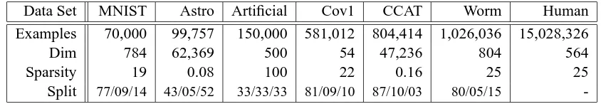
Data Set MNIST Astro Artificial Cov1 CCAT Worm Human
Examples 70,000 99,757 150,000 581,012 804,414 1,026,036 15,028,326
Dim 784 62,369 500 54 47,236 804 564
Sparsity 19 0.08 100 22 0.16 25 25
Split 77/09/14 43/05/52 33/33/33 81/09/10 87/10/03 80/05/15
-Table 2: Summary of the data sets used in the experimental evaluation. Sparsity denotes the aver-age number of non-zero elements of a data set in percent. Split describes the size of the train/validation/test sets in percent.
These data sets have been used and are described in detail in Joachims (2006), Shwartz et al. (2007) and Franc and Sonnenburg (2008a). The Covertype, Astrophysics and CCAT data sets were provided to us by Shai Shalev-Shwartz and should match the ones used in Joachims (2006). The Worm splice data set was provided by Gunnar R¨atsch. We did not apply any extra preprocessing to these data sets.4
The artificial data set was generated from two Gaussian distributions with different diagonal covariance matrices of multiple scale. Unless otherwise stated, experiments were performed on a 2.4GHz AMD Opteron Linux machine. We disabled the bias term in the comparison. As stopping conditions we use the defaults:εlight=εgpdt =0.001,εper f =0.1 andεbmrm=0.001.For OCAS we used the same stopping condition that is implemented in SVMperf , that is,F(w)−Ft(w)
C ≤
εper f 100 =10
−3.
Note that theseεhave very different meanings denoting the maximum KKT violation for SVMlight,
the maximum tolerated violation of constraints for SVMperf and for BMRM the relative duality gap. For SGD we fix the number of iterations to 10 and for Pegasos we use 100/λ, as suggested in Shwartz et al. (2007). For the regularization parameter C and λ we use the following relations: λ=1/C,Cper f =C/100, Cbmrm=C and Clight =Cm. Throughout the experiments we use C as a shortcut for Clight.5
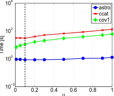
Influence of the Hyper-parameter µ on the Speed of Convergence In contrast to the standard CPA, OCAS has a single hyper-parameter µ (see Section 3). The value of µ determines the point
wct =wbt(1−µ) +wtµ at which the new cutting plane is selected. The convergence proof (see Theo-rem 2) requires µ to be from the interval(0,1], however, the theorem does not indicate which value is the optimal one. For this reason, we empirically determined the value of µ.
For varying µ∈ {0.01,0.05,0.1, . . . ,1} we measured the time required by OCAS to train the classifier on the Astro, CCAT and Cov1 data sets. The regularization constant C was set to the
3. Data sets found at: Worm and Humanhttp://www.fml.tuebingen.mpg.de/raetsch/projects/lsmkl, Cov1 http://kdd.ics.uci.edu/databases/covertype/covertype.html, CCAT http://www.daviddlewis.com/ resources/testcollections/rcv1/, MNISThttp://yann.lecun.com/exdb/mnist/.
4. However, we noted that the Covertype, Astro-ph and CCAT data set already underwent preprocessing because the latter two havekxik2=1.
5. The exact cmdlines are: svm perf learn -l 2 -m 0 -t 0 --b 0 -e 0.1 -cCper f, pegasos -lambda λ -iter 100/λ -k 1, svm learn -m 0 -t 0 -b 0 -e 1e-3 -c Clight, bmrm-train -r 1 -m 10000 -i
optimal value for the given data set. Figure 4 shows the results. For Astro and CCAT the optimal value is µ=0.1 while for Cov1 it is µ=0.01. For all three data sets the training time does not change significantly within the interval(0,0.2). Thus we selected µ=0.1 to be the best value and we used this setting in all remaining experiments.
0 0.2 0.4 0.6 0.8 1 10−2
100 102 104
µ
Time [s]
astro ccat cov1
Figure 4: Training time vs. value of the hyper-parameter µ of the OCAS solver measured on the Astro, CCAT and Cov1 data sets. The value µ=0.1 (dash line) is used in all remaining experiments.
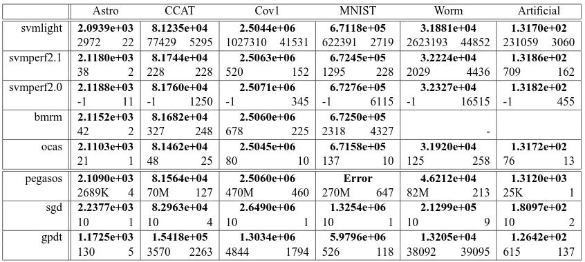
Training Time and Objective For Optimal C We trained all methods on all except the human splice data set using the training data and measured training time (in seconds) and computed the unconstrained objective value F(w)(cf. Equation 11).
The results are displayed in Table 3. The proposed method—OCAS—consistently outperforms all its competitors in the accurate solver category on all benchmark data sets in terms of training time while obtaining a comparable (often the best) objective value. BMRM and SVMperf implement the same CPA algorithm but due to implementation-specific details, results can be different. Our implementation of CPA gives very similar results (not shown).6 Note that for SGD, Pegasos (and SVMper f 2.0—not shown), the objective value sometimes deviates significantly from the true ob-jective. As a result, the learned classifier may differ substantially from the optimal parameter w∗. However, as training times for SGD are significantly below all others, it is unclear whether SGD achieves the same precision using less time with further iterations. An answer to this question is given in the next paragraph.
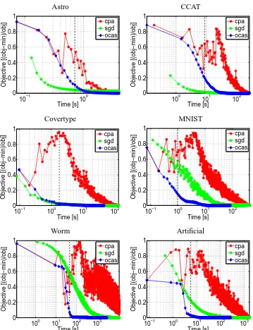
Speed of Convergence (Time vs. Objective) To address this problem we re-ran the best meth-ods, CPA, OCAS and SGD, recording intermediate progress, that is, in the course of optimization record time and objective for several time points. The results are shown in Figure 5. OCAS was stopped when reaching the maximum time or a precision of 1−F(w∗)/F(w)≤10−6 and in all cases achieved the minimum objective. In three of the six data sets, OCAS not only, achieves the
Astro CCAT Cov1 MNIST Worm Artificial
svmlight 2.0939e+03 8.1235e+04 2.5044e+06 6.7118e+05 3.1881e+04 1.3170e+02
2972 22 77429 5295 1027310 41531 622391 2719 2623193 44852 231059 3060
svmperf2.1 2.1180e+03 8.1744e+04 2.5063e+06 6.7245e+05 3.2224e+04 1.3186e+02
38 2 228 228 520 152 1295 228 2029 4436 709 162
svmperf2.0 2.1188e+03 8.1760e+04 2.5071e+06 6.7276e+05 3.2327e+04 1.3182e+02
-1 11 -1 1250 -1 345 -1 6115 -1 16515 -1 455
bmrm 2.1152e+03 8.1682e+04 2.5060e+06 6.7250e+05
42 2 327 248 678 225 2318 4327
-ocas 2.1103e+03 8.1462e+04 2.5045e+06 6.7158e+05 3.1920e+04 1.3172e+02
21 1 48 25 80 10 137 10 125 258 76 13
pegasos 2.1090e+03 8.1564e+04 2.5060e+06 Error 4.6212e+04 1.3120e+03
2689K 4 70M 127 470M 460 270M 647 82M 213 25K 1
sgd 2.2377e+03 8.2963e+04 2.6490e+06 1.3254e+06 2.1299e+05 1.8097e+02
10 1 10 4 10 1 10 1 10 9 10 2
gpdt 1.1725e+03 1.5418e+05 1.3034e+06 5.9796e+06 1.3205e+04 1.2642e+02
130 5 3570 2263 4844 1794 526 118 38092 39095 615 137
Table 3: Training time for optimal C comparing OCAS with other SVM solvers. ”-” means not converged, blank not attempted. Shown in bold is the unconstrained SVM objective value Eq. (11). The two numbers below the objective value denote the number of iterations (left) and the training time in seconds (right). Lower time and objective values are better. All methods solve the unbiased problem. As convergence criteria, the standard settings de-scribed in Section 4.1.1 are used. On MNIST Pegasos ran into numerical problems. OCAS clearly outperforms all of its competitors in the accurate solver category by a large mar-gin achieving similar and often the lowest objective value. The objective value obtained by SGD and Pegasos is often far away from the optimal solution; see text for a further discussion.
best objective as expected at a later time point, but already from the very beginning. Further analysis made clear that OCAS wins over SGD in cases where large Cs were used and thus the optimization problem is more difficult. Still, plain SGD outcompetes even CPA. One may argue that, practi-cally, the true objective is not the unconstrained SVM-primal value (11) but the performance on a validation set, that is, optimization is stopped when the validation error does not change. This has been discussed for leave-one-out in Franc et al. (2008) and we—to some extent—agree with this. One should, however, note that in this case one does not obtain an SVM but some classifier instead. A comparison should not then be limited to SVM solvers but should also be open to any other large scale approach, like online algorithms (e.g., perceptrons). We argue that to compare SVM solvers in a fair way one needs to compare objective values. We therefore ran Pegasos using a larger number of iterations on the Astro and splice data sets. On the Astro data set, Pegasos sur-passed the SVMlightobjective after 108iterations, requiring 228 seconds. SVMlight, in comparison, needed only 22 seconds. Also, on the splice data set we ran Pegasos for 1010iterations, which took 13,000 seconds and achieved a similar objective as that of SVMper f 2.0, requiring only 1224 sec-onds. Finally, note that, although BMRM, SVMperfand our implementation of CPA solve the same equivalent problem using the CPA, differences in implementations lead to varying results.7Since it 7. Potentially due to a programming error in this pre-release of BMRM, it did not show convergence on the splice data
Astro CCAT
10−1 100
0 0.2 0.4 0.6 0.8 1 Time [s] Objective [(obj−min)/obj] cpa sgd ocas
100 101 102 0 0.2 0.4 0.6 0.8 1 Time [s] Objective [(obj−min)/obj] cpa sgd ocas Covertype MNIST
10−1 100 101 102
0 0.2 0.4 0.6 0.8 1 Time [s] Objective [(obj−min)/obj] cpa sgd ocas
10−1 100 101 102 0 0.2 0.4 0.6 0.8 1 Time [s] Objective [(obj−min)/obj] cpa sgd ocas Worm Artificial
100 101 102 103 0 0.2 0.4 0.6 0.8 1 Time [s] Objective [(obj−min)/obj] cpa sgd ocas
10−1 100 101 102 103 0 0.2 0.4 0.6 0.8 1 Time [s] Objective [(obj−min)/obj] cpa sgd ocas
is still interesting to see how the methods perform w.r.t. classification performance, we describe the analysis under this criterion in the next paragraph.
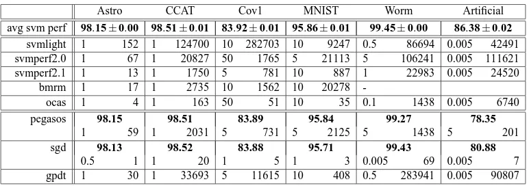
Time to Perform a Full Model Selection When using SVMs in practice, their C parameter needs to be tuned during model selection. We therefore train all methods using different settings8for C on the training part of all data sets, evaluate them on the validation set and choose the best model to do predictions on the test set. As the performance measure, we use the area under the receiver operator characteristic curve (auROC) (Fawcett, 2003). Results are displayed in Table 4.
Astro CCAT Cov1 MNIST Worm Artificial
avg svm perf 98.15±0.00 98.51±0.01 83.92±0.01 95.86±0.01 99.45±0.00 86.38±0.02
svmlight 1 152 1 124700 10 282703 10 9247 0.5 86694 0.005 42491
svmperf2.0 1 67 1 20827 50 1765 5 21113 5 106241 0.005 111621
svmperf2.1 1 13 1 1750 5 781 10 887 1 22983 0.005 24520
bmrm 1 17 1 2735 10 1562 10 20278
-ocas 1 4 1 163 50 51 10 35 0.1 1438 0.005 6740
pegasos 98.15 98.51 83.89 95.84 99.27 78.35
1 59 1 2031 5 731 5 2125 5 1438 5 201
sgd 98.13 98.52 83.88 95.71 99.43 80.88
0.5 1 1 20 1 5 1 3 0.005 69 0.005 7
gpdt 1 30 1 33693 5 11615 10 408 0.5 283941 0.005 90807
Table 4: Model selection experiment comparing OCAS with other SVM solvers. ”-” means not converged, blank not attempted. Shown in bold is the area under the receiver operator characteristic curve (auROC) obtained for the best model chosen based on model selection over a wide range of regularization constants C. In each cell, numbers on the left denote the optimal C, numbers on the right the training time in seconds to perform the whole model selection. Because there is little variance, for accurate SVM solvers only the mean and standard deviation of the auROC are shown. SGD is clearly fastest achieving similar performance for all except the artificial data set. However, often a C smaller than the ones chosen by accurate SVMs is selected—an indication that the learned decision function is only remotely SVM-like. Among the accurate solvers, OCAS clearly outperforms its competitors. It should be noted that training times for all accurate methods are dominated by training for large C (see Table 3 for training times for the optimal C). For further discussion see the text.
Again, among the accurate methods OCAS outperforms its competitors by a large margin, fol-lowed by SVMperf . Note that for all accurate methods the performance is very similar and has little variance. Except for the artificial data set, plain SGD is clearly fastest while achieving a sim-ilar accuracy. However, the optimal parameter settings for accurate SVMs and SGD are different. Accurate SVM solvers use a larger C constant than SGD. For a lower C, the objective function is dominated by the regularization termkwk. A potential explanation is that SGD’s update rule puts more emphasis on the regularization term, and SGD, when not run for a large number of iterations, does imply early stopping.
Our suggestion for practitioners is to use OCAS whenever a reliable and efficient large-scale solver with proven convergence guarantees is required. This is typically the case when the solver is
102 103 104 105 106 10−2
100 102
Time [s]
Dataset Size cpa
sgd ocas linear
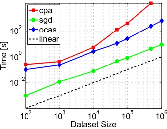
Figure 6: This figure displays how the methods scale with data set size on the Worm splice data set. The slope of the “lines” in this figure denotes the exponent e in
O
(me),where the black line denotes linear effortO
(m).to be operated by non-expert users who know little (or nothing) about tuning the hyper-parameters of the optimization algorithm. Therefore, as long as the full data set fits into memory, we recommend OCAS. Otherwise, if sub-sampling is not an option, online approximative solvers like SGD are the only viable way to proceed.
Effects of Parallelization As OCAS training times are very low on the above data sets, we also apply OCAS to the 15 million human splice data set. Using a 2.4GHz 16-core AMD Opteron Linux machine, we run OCAS using C=0.0001 on 1 to 16 CPUs and show the accumulated times for each of the subtasks, the total training time and the speedup w.r.t. the single CPU algorithm in Table 5. Also shown is the accumulated time for each of the threads. As can be seen—except for the
line-CPUs 1 2 4 8 16
speedup 1 1.77 3.09 4.5 4.6
line search (s) 238 184 178 139 117
at (s) 270 155 80 49 45
output (s) 2476 1300 640 397 410
total (s) 3087 1742 998 684 671
Table 5: Speedups due to parallelizing OCAS on the 15 million human splice data set.
search—computations distribute nicely. Using 8 CPU cores the speedup saturates at a factor of 4.5, most likely as memory access becomes the bottleneck (for 8 CPUs output computation creates a load of 28GB/s just on memory reads).
4.1.2 EVALUATION ON CHALLENGE DATA
In this section, we use the challenge data sets and follow the challenge protocol to compare OCAS to the best-performing methods, which were LaRank (Bordes et al., 2007) and LibLinear (Fan et al., 2008). To this end, we apply OCAS to the challenge data sets Alpha, Gamma and Zeta following the challenge protocol for the SVM track.
The data sets are artificially generated based on a mixture of Gaussians and have certain prop-erties (see Table 6): The Alpha data set is separable with a large margin using quadratic features.
Optimal Number of examples
Data Set Model training testing validation Dim. Description Alpha quadratic 500,000 300,000 100,000 500 well separable Gamma semi-quadratic 500,000 300,000 100,000 500 Multiscale low var.
Zeta linear 500,000 300,000 100,000 2000 Intrinsic dim. 400
Table 6: Summary of the three challenge data sets used: Alpha, Gamma, Zeta.
The Gamma data set is well separable too, but contains features living on different scales. Fi-nally, the optimal model for Zeta is a linear classifier—of its 2,000 features 1,600 are nuisance dimensions. The challenge protocol requires training on the unmodified data sets with C=0.01 and precisionε=0.01.To measure convergence speed, objective values are measured while train-ing. The second challenge experiment simulates model selection by training for different C∈ {0.0001,0.001,0.01,0.1,1,10}.
The left column in Figure 7 displays the course of convergence of the three methods. While OCAS is quite competitive on Gamma and Zeta in this experiment, it is slower on Alpha. It should also be noted that OCAS, in contrast to the online-style algorithms LaRank and LibLinear, has to do a full pass through the data in each iteration. However, it usually requires very few iterations to obtain precise solutions.
In the simulated model selection experiment (right column of Figure 7), OCAS performs well for low values of C on all data sets. However, at first glance it is competitive for large values of C only on Zeta. Investigating objective values on Gamma for LibLinear, we noticed that they signifi-cantly deviate (objective values much larger, deviation by 50% for C=10) from LaRank/OCAS for C∈ {1,10}.Still, on Alpha OCAS is slower.
4.2 Comparison of Linear Multi-Class SVMs
In this section, we compare the proposed multi-class SVM solver OCAM described in Section 3.2 with class CPA (CPAM). We consider the Crammer and Singer (2001) formulation of multi-class SVMs which corresponds to the minimization of the following convex objective,
F(w):=1 2kwk
2+C
m m
∑
i=1max
y∈Y [[yi6=y]] +hwy−wyi,xii
, (19)
Alpha
10−1 100 101 102 3700 3800 3900 4000 4100 4200 4300 4400 4500 4600
CPU Time [s]
Objective
larank liblinear ocas
10−5 10−4 10−3 10−2 10−1 100 101 0 20 40 60 80 100 120 140 160 180 C
CPU Time [s]
larank liblinear ocas
Gamma
100 101 102 103 2200 2400 2600 2800 3000 3200 3400
CPU Time [s]
Objective
larank liblinear ocas
100−5 10−4 10−3 10−2 10−1 100 101 500 1000 1500 2000 2500 3000 3500 4000 4500 C
CPU Time [s]
larank liblinear ocas
Zeta
100 101 102 4985 4990 4995 5000 5005 5010
CPU Time [s]
Objective
larank liblinear ocas
10−5 10−4 10−3 10−2 10−1 100 101 0 50 100 150 200 250 C
CPU Time [s]
larank liblinear ocas
We implemented OCAM and CPAM in C, exactly according to the description in Section 3.2. Both implementations use the Improved Mitchel-Demyanov-Malozemov algorithm (Franc, 2005) as the core QP solver and they use exactly the same functions for the computation of cutting planes and classifier outputs. The implementation of both methods is freely available for download as part of LIBOCAS (Franc and Sonnenburg, 2008b). The experiments are performed on an AMD Opteron-based 2.2GHz machine running Linux.
In the evaluation we compare OCAM with CPAM to minimize programming bias. In addition, we perform a comparison with SVMmulti−classv2.20 later in Section 5.2.
We use four data sets with inherently different properties that are summarized in Table 7. The Malware data set is described in Section 5.2. The remaining data sets, MNIST, News20 and Sector, are downloaded fromhttp://www.csie.ntu.edu.tw/˜cjlin/libsvmtools/datasets/multiclass. html. We used the versions with the input features scaled to the interval[0,1]. Each data set is ran-domly split into a training and a testing part.
features number of num. of examples number of type classes training testing
Malware 3,413 dense 14 3,413 3,414
MNIST 780 dense 10 60,000 10,000
News20 62,060 sparse 20 15,935 3,993
Sector 55,197 sparse 105 6,412 3,207
Table 7: Multi-class data sets used in the comparison of OCAM and CPAM.
Malware MNIST News20 Sector
error time error time error time error time Standard CPAM 10.25 12685 7.07 15898 14.45 7276 5.58 12840 Proposed OCAM 10.16 1705 7.08 5387 14.45 1499 5.61 3970
speedup 7.4 3.0 4.9 3.2
Table 8: Comparison of OCAM and CPA on a simulated model selection problem. The reported time corresponds to training over the whole range of regularization constants Cs. The error is the minimal test classification over the classifiers trained with different Cs.
In the first experiment, we train the multi-class classifiers on training data with a range of regularization constants C ={100,101, . . . ,107} (for Malware C={100, . . . ,108} since the op-timal C=107 is the boundary value). Both solvers use the same stopping condition (10) with
ε=0.01F(w). We measure the total time required for training over the whole range of Cs and the
best classification error measured on the testing data. Table 8 summarizes the results. While the classification accuracy of OCAM and CPAM are comparable, OCAM consistently outperforms the standard CPAM in terms of runtime, achieving speedup of factor from 3 to 7.4.
Malware
100 101 102 103 0 0.2 0.4 0.6 0.8 1 time [s] Objective [(obj−min)/obj] OCAM CPAM
102 103 104
100 101 102 103
# of examples
time [s] OCAM
CPAM O(x)
100 0 102 104 106 108 2000 4000 6000 8000 10000 12000 C time [s] OCAM CPAM MNIST
100 101 102 103 0 0.2 0.4 0.6 0.8 1 time [s] Objective [(obj−min)/obj] OCAM CPAM
102 103 104 105 10−1
100 101 102 103
# of examples
time [s]
OCAM CPAM O(x)
100 0 102 104 106 108 2000 4000 6000 8000 10000 12000 C time [s] OCAM CPAM News20
100 101 102 0 0.2 0.4 0.6 0.8 time [s] Objective [(obj−min)/obj] OCAM CPAM
102 103 104 100
101 102
# of examples
time [s]
OCAM CPAM O(x)
100 102 104 106 108 0 2000 4000 6000 C time [s] OCAM CPAM
Figure 8: Results of the standard CPAM and the proposed OCAM on the Malware, MNIST and News20 data sets. The left column of figures displays the unconstrained SVM objec-tive (19) w.r.t. SVM training time. The middle column displays the training time as a function of the number of examples. In both experiments C was fixed to its optimal value as determined in model selection. The right column shows the training time for different Cs. See text for a discussion of the results.
5. Applications
In this section we attack two real-world applications. First, in Section 5.1, we apply OCAS to a human acceptor splice site recognition problem. Second, in Section 5.2, we use OCAM for learning a behavioral malware classifier.
5.1 Human Acceptor Splice Site Recognition
To demonstrate the effectiveness of our proposed method, OCAS, we apply it to the problem of human acceptor splice site detection. Splice sites mark the boundaries between potentially protein-coding exons and (non-protein-coding) introns. In the process of translating DNA to protein, introns are excised from pre-mRNA after transcription (Figure 9). Most splice sites are so-called canonical splice sites that are characterized by the presence of the dimersGTandAGat the donor and acceptor sites, respectively.
Figure 9: The major steps in protein synthesis. In the process of converting DNA to messenger RNA, the introns (green) are spliced out. Here we focus on detecting the so-called ac-ceptor splice sites that employ the AGconsensus and are found at the “left-hand side” boundary of exons. Figure taken from (Sonnenburg, 2002).
However, the occurrence of the dimer alone is not sufficient to detect a splice site. The classifi-cation task for splice site sensors, therefore, consists in discriminating true splice sites from decoy sites that also exhibit the consensus dimers. Assuming a uniform distribution of the four bases, adenine (A), cytosine (C), guanine (G) and thymine (T), one would expect 1/16th of the dimers to contain the AGacceptor splice site consensus. Considering the size of the human genome, which consists of about 3 billion base pairs, this constitutes a large-scale learning problem (the expected number ofAGs is 180 million).