Automatic PCA Dimension Selection for High Dimensional Data and Small Sample Sizes

Automatic PCA Dimension Selection for High Dimensional Data and

Small Sample Sizes

David C. Hoyle [email protected]

North West Institute for BioHealth Informatics,

University of Manchester, Faculty of Medical and Human Sciences, University Place (East), Oxford Rd., Manchester, M13 9PL, UK.

Editor: Chris Williams

Abstract

Bayesian inference from high-dimensional data involves the integration over a large number of model parameters. Accurate evaluation of such high-dimensional integrals raises a unique set of issues. These issues are illustrated using the exemplar of model selection for principal component analysis (PCA). A Bayesian model selection criterion, based on a Laplace approximation to the model evidence for determining the number of signal principal components present in a data set, has previously been show to perform well on various test data sets. Using simulated data we show that for d-dimensional data and small sample sizes, N, the accuracy of this model selection method is strongly affected by increasing values of d. By taking proper account of the contribution to the evidence from the large number of model parameters we show that model selection accuracy is substantially improved. The accuracy of the improved model evidence is studied in the asymptotic limit d_→∞at fixed ratio α=N/d, with α<1. In this limit, model selection based upon the improved model evidence agrees with a frequentist hypothesis testing approach.

Keywords: PCA, Bayesian model selection, random matrix theory, high dimensional inference

1. Introduction

Clearly selection of the correct number of principal components is crucial to the success of PCA in representing a data set. Identification of the appropriate signal dimensionality is just a model selection process to which the techniques of Bayesian model selection can be applied via a suitable approximation of the Bayesian evidence (MacKay, 1992). What is the most suitable method of approximating the evidence for high-dimensional data and what are the inherent problems? These are the research questions we address and a roadmap for the paper is given below,

•In Section 2 we motivate why high-dimensional small sample size data sets present a challenge for Bayesian model selection.

•In Section 3 we summarize the behaviour of the eigenvectors and eigenvalues of sample co-variance matrices formed from high-dimensional small sample size data sets.

• In Section 4.1 we review the formalism of Bayesian model selection for PCA, and evalu-ate through simulation the model selection accuracy of an existing approximation to the Bayesian evidence.

•In Section 4.2 we develop an improved approximation to the Bayesian evidence specifically for high dimensional data.

•In Section 5 we evaluate the asymptotic properties of the improved approximation to the model evidence.

• In Section 6 the model selection performance of the improved approximation to the model evidence is compared with a frequentist hypothesis testing approach to model selection.

2. The Challenge of High-Dimensional Data for Bayesian Model Selection

A number of Bayesian formulations of PCA have followed from the probabilistic formulation of Tipping and Bishop (1999a), with the necessary marginalization being approximated through both Laplace approximations (Bishop, 1999a; Minka, 2000, 2001a) and variational bounds (Bishop, 1999b). More recently, work within the statistics research community has used a Bayesian vari-ational approach to derive an explicit conditional probability distribution for the signal dimension given the data ( ˇSm´ıdl and Quinn, 2007). However, these results have only been tested on low di-mensional data with relatively large sample sizes. A somewhat more tractable expression for the signal dimension posterior was also obtained by Minka (2000, 2001a) and it is that Bayesian for-mulation of PCA that we draw upon. By performing a Laplace approximation (Wong, 1989), that is, expanding about the maximum posterior solution, Minka derived an elegant approximation to the probability, the model evidence p(D_|k), of observing a data set D given the number of principal components k (Minka, 2000, 2001a). The signal dimensionality of the given data set is then esti-mated by the value of k that maximizes p(D_|k). As with any Bayesian model selection procedure, if the data has truly been generated by a model of the form proposed, then one is guaranteed to select the correct model dimensionality as the sample increases to an infinite size. Minka’s dimensionality selection method performs well when tested on data sets of moderate size and dimensionality. In-deed, the Laplace approximation incorporates the leading order term in an asymptotic expansion of the Bayesian evidence, with the sample size N playing the role of the ‘large’ parameter, and so we would expect the Laplace approximation to be increasingly accurate as N_→∞. In real-world data sets, such as those emanating from molecular biology experiments, the number of variables d is often very much greater than the sample size N, with d_∼104_{yet N∼10 or N∼10}2_{not uncommon}

approximation to be appropriate. However, though retaining only a small number of terms from the asymptotic expansion of the evidence would be increasingly accurate as N_→∞, individual expan-sion coefficients may be significant due to the large data dimenexpan-sionality d. This suggests that for real finite sample size data sets, higher order terms in the asymptotic expansion not encapsulated within the Laplace approximation will make significant contributions to the evidence, and model selection based upon a simplistic application of the Laplace approximation will perform poorly. What then defines a ‘large’ sample size N is clearly dependent on the data dimensionality d. We would expect the conjectures about the previously derived Laplace approximation to the evidence to be increasingly true when the data dimensionality is very much larger than the sample size, that is,

Nd, the situation encountered for many modern data sets. For high dimensional data, rather than

considering the evidence to be close to its value obtained in the asymptotic limit N_→∞at fixed d, it may be more appropriate to consider the evidence as being close to its value in the distinguished limit d,N_→∞at fixedα=N/d. Within this paradigm, developing a suitable Gaussian approxi-mation requires us to identify all contributions to the evidence that would scale extensively, that is increase linearly with N, as N,d_→∞at fixedα. This would be increasingly important forα<1, where the contribution to the evidence resulting from many features can be significant. Ideally we should re-formulate the evidence as an integration over a set of variables which remains finite in number in the distinguished limit.

To be more explicit, consider that the Bayesian approach to model selection in PCA starts from the probability p(D_|k,θ)p(θ_|k)and integrates over the model parametersθto obtain the evidence

p(D_|k). This integration is often evaluated by the aforementioned Laplace approximation -

expan-sion about the maximum of p(D_|k,θ)p(θ_|k)and evaluation of the consequent tractable Gaussian integrals. For high-dimensional data the model parameters may consist of a small set of parameters,

θk, of order of the signal dimensionality k, and a much larger set of parameters, θd, of order of

the data dimensionality. For example, the latter may be the principal vectors, in the d-dimensional space, that form part of the model. Overall we can writeθ= (θd,θk). Integration overθd provides

a significant contribution to p(D_|k) due simply to the large number of individual model param-eters that we are integrating over. In this scenario, the values of θk obtained from maximizing R

p(D_|k,θd,θk)p(θd,θk|k)dθd and p(D|k,θd,θk)p(θd,θk|k)do not coincide. In fact for large

val-ues of d they may be significantly different. The more accurate estimates ofθkare naturally obtained

from the maximum ofR

p(D_|k,θd,θk)p(θd,θk|k)dθd, and consequently the more accurate estimates

of the evidence p(D_|k)are obtained by expanding about this maximum.

The distorting effects of high dimensionality upon covariance matrix eigenvalue spectra and eigenvectors are well known from random matrix theory (RMT) studies (Johnstone, 2006). The RMT studies inform us about the expected sample covariance eigenvalue spectrum in the limit d_→∞(at fixedα), and consequently the limits of any model selection procedure based upon the observed eigenvalue spectra. As PCA is based upon the eigenvalues and eigenvectors of ˆC, under-standing their behaviour for small sample sizes and high data dimensions is key to underunder-standing the behaviour of the existing model selection criterion, including the Bayesian model selection ap-proach of Minka. Results from RMT studies are summarized in Section 3.

3. High-Dimensional Sample Covariance Matrices

We envisage a scenario where one has N, d-dimensional data vectorsξµ,µ=1, . . . ,N, with sample

eigen-values ofCwe denote byΛi,i=1, . . . ,d. The sample data vectorsξµcontain both signal and noise

components so we represent,

C=σ2I+

S

∑

m=1 σ2_A

mBmBTm , BTmBm0 =δ_mm0 , A_m≥0∀m, (1)

corresponding to a population covariance C that contains a small number, S, of orthogonal sig-nal components,_{Bm}Sm=1, but that is otherwise isotropic. Here,σ2represents the variance of the

additive noise component of the sample data vectors. Such models have been termed “spiked” co-variance models within the statistics research literature (Johnstone, 2001), due to the small number ofδ-function spikes in the population covariance eigenspectrum. In this case the population eigen-values areΛi=σ2(1+Ai),i≤S andΛi=σ2,i>S. The signal strengthsσ2Ammerely determine

the population covariance eigenvalues corresponding to signal directions, and so the number of sig-nal components S is commonly estimated by some process of inspection of the ordered eigenvalues

λi,i=1, . . . ,d, of the sample covariance matrix ˆC =N−1∑µ(ξµ−ξ¯)(ξµ−ξ¯)T.

When the sample size is greater than the dimensionality, that is, N>d, the sample covariance eigenvaluesλi may be reasonable estimators of the population covariance eigenvalues Λi, and

in-deed are asymptotically unbiased estimators, that is,λi→Λi as N→∞for fixed dimensionality d

(Anderson, 1963). However, for small sample sizes N_≤d the sample covariance ˆCis singular with a d₋N+1 degenerate zero eigenvalue. Similarly, the non-zero sample covariance eigenvalues,

λi,i=1, . . . ,N−1, can display considerable bias. This is reflected in the expected eigenspectrum,

ρ(λ), which is simply defined as the expectation over data sets of the empirical eigenvalue density,

ρ(λ) = Eξ

1 d

d

∑

i=1

δ(λ₋λi)

!

.

Hereδ(x)is the Diracδ-function, and we have used Eξ(·)to denote expectation over the ensemble

of sample data sets. The empirical eigenvalue density is considered to be a self-averaging quantity, such that as N→∞the eigenvalue density from any individual sample covariance matrix is well represented by the ensemble average. Therefore, for large sample covariance matrices studying the behaviour of the expected sample covariance eigenvalue distribution provides us with insight into the behaviour of individual sample covariance matrices and consequently the behaviour of any model selection algorithms based upon the sample covariance eigenvalues.

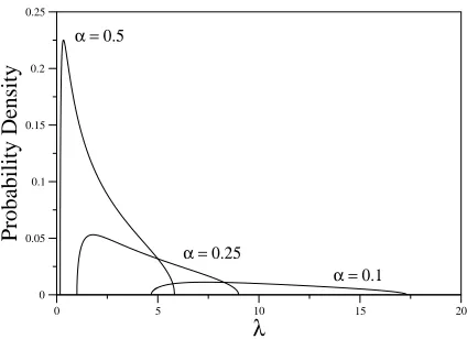
When no signal components are present, that is,C=σ2_{I, and in the limit d→∞withα=N/d}

fixed, the expected distribution of sample eigenvalues tends to the Mar ˇcenko-Pastur distribution (Marˇcenko and Pastur, 1967),

ρ(λ) = ρbulk(λ) = (1−α)Θ(1−α)δ(λ)

+ α

2πλσ2

p

max[0,(λ₋λmin)(λmax−λ)] , (2)

whereλmax=σ2(1+α−

1

2)2,λ_min=σ2(1−α− 1

2)2, andΘ(x)is the Heaviside step function. Figure 1 shows examples of the Marˇcenko-Pastur distribution for different values ofα. It should be noted that although the mean sample eigenvalue is an unbiased estimator ofσ2_{, that is,}R∞

0−dλλρbulk(λ) =σ2,

the individual non-zero sample covariance eigenvalues lie in the interval[λmin,λmax]and so forα<1

0 5 10 15 20

λ

0 0.05 0.1 0.15 0.2 0.25

Probability Density

α = 0.5

α = 0.25

α = 0.1

Figure 1: The Marˇcenko-Pastur limiting distribution for sample covariance eigenvalues, at α = 0.1,0.25,0.5. In all cases σ2 =1. We have shown only the part of the distribution pertaining to non-zero eigenvalues. Forα<1 there is also aδ-function peak atλ=0 due to the singular nature of the sample covariance matrix - see main text.

Hoyle and Rattray (2004a) studied the expected behaviour of the sample covariance eigenvalue spectrum for “spiked” covariance models in the asymptotic limit d_→∞at fixedα, by using tech-niques from statistical physics. Similar results have been obtained within the statistics research community (Baik and Silverstein, 2006). As the addition of a small number, S, of signal directions provides a relatively small perturbation to an isotropic population covariance, the majority, or bulk of eigenvalues are still distributed according to the Marˇcenko-Pastur law. For this reason we have usedρbulk(λ) to denote the Marˇcenko-Pastur distribution. For the “spiked” covariance models of

Equation (1) the expected eigenvalue distributionρ(λ)is modified fromρbulk(λ). At finite but large

values of d and N the expected sample covariance eigenvalue density can be approximated by,

ρ(λ) = (1₋α)Θ(1₋α)δ(λ) + 1 d

S

∑

m=1

δ(λ₋λu(Am))Θ(α−A−m2)

+ 1₋d−1

S

∑

m=1

Θ(α₋A−_m2) !

α

2πλσ2

p

max[0,(λ₋λmin)(λmax−λ)] , (3)

whereλu(A) =σ2(1+A)(1+ (αA)−1). A number of interesting features are present in this

spec-trum. A transition occurs at α=A−2

m , such that for α>A−m2 a sample eigenvalue located at

λ=λu(Am)can be resolved separately from the remaining Marˇcenko-Pastur bulk of eigenvalues.

Thus for S signal components within the “spiked” covariance model we can observe up to S transi-tions in the sample covariance eigenspectrum, on increasingα. The first transition pointα=A−₁2 corresponds to the transition point in learning the leading signal directionB1. The scenario of

considered the behaviour (as d→∞at fixedα) of the expectation value of R2₁, where R1=B1·J1is

the overlap between the first principal componentJ1of the sample covariance andB1. One observes

the phenomenon of retarded learning whereby R2₁=0 forα<A−₁2and R2₁>0 forα>A−₁2. This has been generalized to learning multiple orthogonal signals and one observes a separate retarded learn-ing transition atα=A−_m2 for each of the overlaps R2_m= (Bm·Jm)2, whereJmis the mth principal

component (Hoyle and Rattray, 2007). That the ability to detect the signal components is reflected in the sample covariance eigenvalue structure (with retarded learning transitions coinciding with transitions in the eigenspectrum) demonstrates the utility of the sample covariance eigenspectrum for model selection. It also highlights that if the true signal dimensionality is S then asymptotically we have at most only S sample covariance eigenvalues separated from the Mar ˇcenko-Pastur bulk distribution, dependent on the value ofα. If, for the given value ofα, we have ˆS eigenvalues sepa-rated from the Marˇcenko-Pastur bulk distribution, then the asymptotic equivalence of the observed sample covariance eigenspectra whenC contains S signals or ˆS_≤S signals means that no correct Bayesian model selection procedure can, asymptotically, select greater than ˆS principal components (applying an Occam’s Razor like argument), since both models are equally capable of explaining the observed eigenspectra. Equally, for sufficiently smallαit is impossible, asymptotically, to dis-tinguish the sample spectrum from one which has been generated from a model containing no signal structure, that is, from a population covarianceC=σ2_{I. Within these constraints placed by the}

ex-pected behaviour of the observed eigenspectra we now attempt to derive a suitable Bayesian model selection procedure that performs well in the distinguished asymptotic limit N,d_→∞at fixedα.

4. Bayesian Model Selection

In this section we summarize the Bayesian model selection procedure for PCA. We start in Section 4.1 by reproducing the formulation of the Bayesian model evidence as outlined by Minka (2000, 2001a) and the subsequent Laplace approximation. In Section 4.2 we re-express the evidence in a form that is more suitable for application of a Gaussian approximation when d,N_→∞at fixed

α<1.

4.1 Laplace Approximation of Minka

The data vectorsξµ are modelled as being drawn from a multi-variate Gaussian distribution with

meanmand covarianceΣ=vI+HHT. ThusΣacts as a model of the true population covariance

C. The matrixH represents the signal considered present in the data and so is modelled as being due to a small number, k, of orthogonal signal componentsui,i=1, . . . ,k. Consequently we set,

H=U(L₋vIk)1/2W , UTU =Ik , WTW =Ik ,

where the columns of the orthonormal matrixU are formed from the vectors ui. The parameter

v provides an estimator of the true population noise level σ2_{. The diagonal matrix L has}

ele-ments li,i=1, . . . ,k, which represent estimators of the population covariance eigenvaluesΛi. The

orthonormal matrix W represents an irrelevant rotation within the subspace and is subsequently eliminated from the calculation. Model selection proceeds via the standard use of Bayes’ theorem,

p(H,m,v_|D) = p(D|H,m,v)p(H,m,v)

The signal dimensionality, k, is implicit in the matrixH. With a non-informative prior, the mean

mcan be integrated out to yield the probability of observing the data set D givenH and v (Minka, 2001a),

p(D_|H,v) = N−d/2(2π)−(N−1)d/2_|HHT+vI_|−(N−1)/2exp

−N₂tr((HHT+vI)−1Cˆ)

.

Given a prior p(U,W,L,v)the evidence for a signal dimensionality k is then,

p(D_|k) =

Z

dUdWdLdv p(D_|U,W,L,v)p(U,W,L,v).

The integration over the elements li, i=1, . . . ,k is restricted to the region li ≥0∀i. Similarly,

the integration over U andW is over the entire space of d_×k and k_×k orthonormal matrices respectively. For the relevant integration over U this is equivalent to integration over the Stiefel manifold Vk(Rd)defined by the set of all orthonormal k-frames inRd (James, 1954) .

Minka chooses a conjugate prior,

p(U,W,L,v) ∝ _|HHT+vI_|−(η+2)/2exp(₋η

2tr((HH

T_+vI)−1_{)), (4)}

where the hyper-parameter η controls the sharpness of the prior. For a non-informative prior η should be small and ultimately we shall takeη_→0+in our resulting approximation to the evidence

p(D_|k). With the prior given in Equation (4) the evidence is Minka (2000, 2001a),

p(D_|k) =

N

Area(Vk(Rd)) Z

dUdLdv_|HHT+vI_|−(N+1+η)/2

× exp(₋N

2tr((HH

T_+vI)−1_{(Cˆ +N−}1_{ηI))), (5)}

with,

N

N−d/2(2π)−(N₋1)d/2 Γ (1

2η+1)(d−k)−1

(η(d−k)/2)

(1

2η+1)(d−k)−1 1

Γ(η/2)k(η/2)

ηk/2 _,

and here 1/Area(Vk(Rd))is the reciprocal of the area of the Stiefel manifold Vk(Rd)(James, 1954),

1 Area(Vk(Rd))

= 2−k

k

∏

i=1

Γ((d₋i+1)/2)π−(d−i+1)/2.

The dependence of

N

ln p(D_|k), and so Minka drops

N

the maximum likelihood case (Tipping and Bishop, 1999a), for a fixed choice, k, of the number of principal components, the maximum posterior estimators for_{ui}ki=1are known to be the

eigenvec-tors of ˆCcorresponding to the k largest eigenvalues of ˆC. Minka approximates the evidence p(D_|k) in Equation (5) using a Laplace approximation, expanding about the maximum posterior solution. The stationary point values of v and_{li}ki=1are denoted by ˆv and{ˆli}ki=1respectively, and are given

by (on takingη→0),

ˆli =

Nλi

N₋1 ' λi , vˆ =

N∑d_j=k+1λj

Within this approximation ˆli provides a point estimate of the ith population covariance eigenvalue

Λi. Forα<1, as we have already commented in the previous section,λi can be highly biased and

consequently a poor point estimate ofΛi. Continuing with the Laplace approximation and setting

m=dk−k(k+1)/2, Minka finds (again after takingη→0),

p(D_|k)_' 1

Area(Vk(Rd)) k

∏

j=1 λj

!−N/2 ˆ

v−N(d−k)/2(2π)(m+k)/2_|A

Z|−1/2N−k/2, (7)

where,

|AZ|=

k

∏

i=1

d

∏

j=i+1

(Λˆ−1

j −Λˆ−i 1)(λi−λj)N.

The estimator ˆΛiis given by ˆΛi=ˆli'λifor i≤k and ˆΛi=v for iˆ >k.

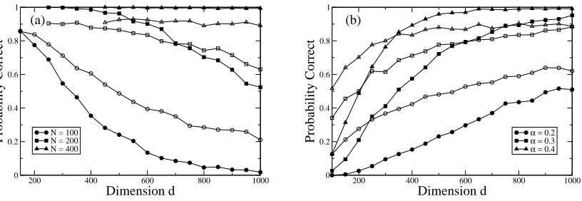
Figure 2 shows simulation estimates of the performance of a model selection criterion based upon the evidence given by Equation (7). We have sampled data vectors ξµ from a population

covariance C containing three signal components. The noise level has been set to σ2=1 and the signal strengths are A2₁=30,A₂2=20,A2₃=10. The simulation results are averages evaluated over 1000 simulated data sets. Plotted in Fig.2(a) is the probability of selecting the correct model dimension against d, for different fixed values of N. As expected the accuracy of the model selection decreases with increasing d, with greater accuracy for larger sample sizes N at a given value of d. Plotted in Fig.2(b) is the probability of selecting the correct model dimension against d, for different fixed values of α. Note that the smallest value studied, α=0.2, is still greater than the retarded learning transition point of the weakest signal component, which occurs atα=A−₃2=0.1.

200 400 600 800 1000

Dimension d

0 0.2 0.4 0.6 0.8 1

Probability Correct

N=100 N = 200 N = 400

(a)

200 400 600 800 1000

Dimension d

0 0.2 0.4 0.6 0.8

Probability Correct

α = 0.2 α = 0.3 α = 0.4

(b)

Figure 2: Probability of correct model selection using the method of Minka. The solid lines provide a guide to the eye. (a) & (b) Plots of model selection accuracy against data dimension d - (a) Fixed values of N, (b) Fixed values ofα. The data is generated with a population covarianceC containing three signal components -see main text for details. Solid sym-bols represent simulation results from the model selection procedure applied to the mean centred data matrix, whilst open symbols represent simulation results from the model selection procedure applied to the transpose of the mean centred data matrix.

4.2 Overlap Method

Although forα<1 the top k eigenvectors of ˆC are the maximum posterior choice of model prin-cipal components_{ui}ki=1, for non-maximum posterior choices ofU one still has a large rotational

degeneracy of the k-frame within the d-dimensional space, which will make a large contribution to the integral in Equation (5). The integrand in Equation (5) can be written in terms of the over-laps Ri j =ui·vj between the model principal components ui,i=1, . . . ,k, and the eigenvectors

vj, j=1, . . . ,N−1, of ˆC that correspond to the non-zero eigenvalues of ˆC. One finds,

|HHT+vI_|−(N+1+η)/2exp(₋N

2tr((HH

T_+vI)−1_{(Cˆ +N}−1_ηI)))

= exp "

−N+1+η

2

k

∑

i=1

ln li+ (d−k)ln v

!

−N

2v

N−1

∑

j=1 λj

+ N

2

k

∑

i=1

(v−1₋l_i−1)

N₋1

∑

j=1

λjR2i j −

ηd 2v +

η

2

k

∑

i=1

(v−1₋l_i−1) #

.

This suggests performing the integration over _{ui}ki=1 in terms of{Ri j}. The volume element

that results from integrating over_{ui}k_i=1 at fixed {Ri j}is detM(d−N−1)/2×Area(Vk(Rd−N+1)),

where the matrix elements Mii0 =δ_ii0−∑_jR_{i j}R_i0_j. For high dimensional spaces we might ex-pect the vectors ui,ui0 to be orthogonal over any high-dimensional subspace, not just the entire

d-dimensional space. Therefore we can approximate the matrix elements by Mii0=δ_ii0(1−∑_jR2_{i j}),

p(D_|k)_'

N

Area(Vk(Rd−N+1))

Area(Vk(Rd)) Z

∏

i j

dRi j Z

∏

d₋N₋1

2

k

∑

i=1

ln1₋

N−1

∑

j=1

R2_{i j−} N+1+η

2

k

∑

i=1

ln li+ (d−k)ln v

!

− _2vN

N−1

∑

j=1 λj +

N 2

k

∑

i=1

(v−1₋l_i−1)

N−1

∑

j=1

λjR2i j −

ηd 2v + η 2 k

∑

i=1

(v−1₋l_i−1) #

. (8)

Approximations to the model evidence can now be made by approximating this integration over the overlap variables_{Ri j}, and consequently this approach is termed the “overlap” method.

For large values of d and N we would expect the integral in Equation (8) to be dominated by the stationary points of the exponent and a Laplace approximation to the integral can be constructed. Denoting stationary point values by ˆv,ˆli,Rˆi j, it is an easy matter to find that, on taking η→0,

stationary points of Equation (8) satisfy for some j,

1₋Rˆ2_{i j} = (vˆ−

1_−ˆl−1

i )Nλj

d−N−1 , Rˆi j0 = 0 , j

0_{6= j.}

The dominant stationary point solution has the overlap between the ithsignal direction estimate,ui

and the ithsample covariance eigenvector,vi, being non-zero, that is, ˆR2ii>0,Rˆ2ii0 =0,∀i6=i0, For j>k the dominant stationary point has ˆR2_{i j}=0. Within this approximation the expectation value of R2_{i j} will be O(N−1_{) due to small fluctuations about this stationary point. However, we}

have an extensive number, that is, proportional to N, of such overlap variables. Thus we expect

∑j>kR2i j ∼1, and consequently the contribution from these small fluctuations cannot be ignored.

The fluctuations in Ri j, for j>k, collectively affect the stationary point behaviour of the overlaps

Ri j for j≤k. To progress we integrate out the fluctuations by setting,

bi=

∑

j>k

R2_{i j},

and perform the integration over_{Ri j}j>kby writing,

Z

∏

i

∏

dRi j =

Z

∏

i

∏

dRi j

∏

i

dbiδ bi −

∑

j>k

R2_{i j} !

.

Using the standard Fourier representation of a Diracδ-function,

δ(x) = 1 2π

Z i∞

−i∞

d p epx,

we obtain,

Z

∏

i

∏

dRi j =

1 (2π)k

Z

∏

i

dbid pi

∏

i

∏

dRi jexp

"

∑

i

pi bi−

∑

j>k

R2_{i j} !#

where the path of integration for pi is between−i∞and+i∞. Combining the integrand in

Equa-tion (9) with the integrand in EquaEqua-tion (8), the integraEqua-tion over_{Ri j}j>k is Gaussian and so easily

performed. We obtain,

Z

dv

Z k

∏

i=1

dlidbid pi

∏

i

∏

dRi jexp

k

∑

i=1

pibi +

1

2(d−N−1)

k

∑

i=1

ln[1₋

k

∑

j=1

R2_{i j−}bi]

−1₂

k

∑

i=1

∑

ln[2pi−N(v−1−li−1)λj]−

N+1

2 "

k

∑

i=1

ln li + (d−k)ln v

#

−N₂v−1

N₋1

∑

j=1 λj +

N 2

k

∑

i=1

(v−1₋l_i−1)

k

∑

j=1 λjR2i j

!

. (10)

With the path of integration for pi being along the imaginary axis the remaining integrals in

Equation (10) are approximated via steepest descent (Wong, 1989). For brevity we give only the solutions to the saddle point equations, with the caret again denoting saddle-point values of the corresponding integration variables,

ˆ

v = N

(N+1)(d₋k) "

N−1

∑

j=1 λj −

k

∑

i=1

(1+N−1)ˆli

#

, (11)

0 = ˆl_i2vˆ−1(1+N−1) ₋ ˆli(λivˆ−1−α−1+1+N−1(k+3)) + λi, (12)

ˆ

R2_ii = 1 ₋ (d−N−1)

N(vˆ−1_−ˆl−1

i )λi

− 1

N

∑

1 (vˆ−1_−ˆl−1

i )(λi−λj)

, (13)

ˆ

R2_{i j} = 0 ,j₆=i, j_≤k,

ˆ

pi =

N 2(vˆ

−1_−ˆl−1

i )λi, (14)

ˆbi = 1 −Rˆ2ii −

(d₋N₋1) N(vˆ−1_−ˆl−1

i )λi

. (15)

Again the saddle-point solution values ˆv and ˆli provide us with point estimates for the

popula-tion noise levelσ2and population signal eigenvalueΛirespectively. Equations (11) and (12) can be

solved efficiently via an iterative process starting from an initial estimate of ˆv=d−1∑jλj.

Obtain-ing real-valued estimates, ˆli, for the population covariance eigenvalues is clearly dependent upon

the quadratic equation in (12) having a non-negative discriminant. In practice, we have interpreted complex-valued estimates ˆli for a particular choice of signal dimensionality k as meaning that the

particular choice for k is not appropriate and should not be considered. From analysis of the asymp-totic behaviour of the “overlap” approximation (see next section) we find that the discriminant of Equation (12) becomes negative for sample covariance eigenvaluesλiwhich are below the edge of

the Marˇcenko-Pastur bulk distribution given in Equation (2), that is,λi<λmax=σ2(1+α−

1 2)2, so that indeed a negative discriminant is consistent with attempting to extract more signal components than can be genuinely distinguished from an isotropic population covariance. In other words com-plex solutions to Equation (12) suggest that the data do not support a model with that number, k, of signal components.

Once solutions for ˆv and_{ˆli}ki=1have been obtained, values for ˆR2ii,pˆi,ˆbifollow from Equations

200 400 600 800 1000 Dimension d 0 0.2 0.4 0.6 0.8 1 Probability Correct

N = 100 N = 200 N = 400

(a)

200 400 600 800 1000

Dimension d 0 0.2 0.4 0.6 0.8 1 Probability Correct

α = 0.2 α = 0.3 α = 0.4

(b)

Figure 3: Plot of model selection accuracy for the “overlap” method. (a)Plot of model selection ac-curacy against data dimension d at fixed values of N. (b)Plot of model selection acac-curacy against data dimension for fixed values ofα. For comparison open symbols represent simulation results from the model selection procedure of Minka applied to the transpose of the mean centred data matrix.

ln p(D_|k) _' N 2

k

∑

i=1

(vˆ−1₋ˆl_i−1)λi −

k

2(d−N−1) + k

d₋N₋1

2 ln

d₋N₋1

N

− d−N−1

2

k

∑

i=1

ln((vˆ−1₋ˆl_i−1)λi) −

k

2(N−k)ln N −

N₋k

2

k

∑

i=1

ln(vˆ−1₋ˆl_i−1)

− 1₂

k

∑

i=1

∑

ln(λi−λj) −

N+1

2

k

∑

i=1

ln ˆli −

N+1

2 (d−k)ln ˆv − N

2vˆ

−1N

∑

j=1 λj

+ k

2(N−k−1)ln 2π + ln

Area(Vk(Rd−N+1))

Area(Vk(Rd))

− 1

2ln detHs

+ 3k+k

2₊₁

2 ln 2π, (16)

whereHsis the Hessian of the exponent in the integrand evaluated at the saddle point. The last two

terms in (16) come from integrating over the small fluctuations about the saddle point. Since the Hessian is of small dimension, and so not strongly dependent on N and d, we subsequently drop the last two terms from our approximation of the log-evidence. The “overlap” approximation to the log-evidence, given in Equation (16), can be used for model selection by selecting the value of k that has the highest value of ln p(D_|k).

pa-rameter values are identical to those in Figure 2. Also reproduced (open symbols) in Fig.3(a) and Fig.3(b) are the simulation estimates of model selection accuracy for Minka’s approximation to the model evidence applied to the transposed mean centred data. From Fig.3(a) it is clear that the “over-lap” model selection criterion only suffers from degradation in performance at significantly higher values of dimension d compared to the approximation to the evidence in Equation (7). Similarly, Fig.3(b) demonstrates the superior model selection accuracy of the “overlap” method for increasing dimensionality d, at fixed values ofα.

5. Asymptotic Analysis

The “overlap” approximation to the model evidence has been developed by applying a steepest descent approximation to the Bayesian evidence that has been re-formulated in terms of integration over variables that remain finite in number in the distinguished asymptotic limit d,N→∞, at fixedα. The “overlap” approximation essentially contains the leading order term of an asymptotic expansion of the evidence in that distinguished limit. It would be expected that the approximation to the model evidence would therefore become increasingly accurate in this limit. Note that this is very different from the traditional large sample limit N _→∞at fixed d, for which Minka’s approximation to the Bayesian evidence will become increasingly accurate. It has been argued that since for many real high-dimensional data setsα1, one would expect that approximations to the model evidence that are accurate in the distinguished limit will have superior model selection accuracy at finite values

of d,N. The simulation results presented in Fig.3 would appear to confirm this. However, more

concrete understanding of the accuracy of the “overlap” method in the distinguished asymptotic limit is required. A theoretical analysis of model selection accuracy in this limit would provide us with a firmer comparison of Minka’s original Laplace approximation and the “overlap” method, in addition to the comparison provided by simulation study in Section 4.2. A number of quantities such as the eigenvalue spectrum are self-averaging in the asymptotic limit, that is, have vanishing sampling variation, so that for large data dimensions, d, the value for a single data set, _{ξµ}, is

well approximated by the ensemble average over data sets. Studying the ensemble expectation, in the asymptotic limit of d_→∞at fixedα, of the “overlap” approximation to the model evidence provides us with insight into its accuracy as a model selection procedure for high dimensional data. From Equation (11) it is evident that ˆv = d−1∑N_j=−₁1λj +O(N−1)as N→∞. Consequently, due

to the self-averaging nature of the sample covariance eigenvalue spectrum, we have that ˆv_→Eξ(λ)

as N_→∞, where we have used Eξ(·)to denote expectation over the ensemble of sample data sets.

We already commented in Section 3 that Eξ(λ) = σ2 in the asymptotic limit N →∞at fixedα,

and so ˆv provides an asymptotically unbiased estimate of the population noise level. Estimates of the population signal eigenvalues are given by _{ˆli}ki=1, and in the distinguished asymptotic limit

solutions to Equation (12) for ˆliare given by,

ˆli =

ˆ v 2

(1+λivˆ−1−α−1)±

q

(1+λivˆ−1−α−1)2 − 4λivˆ−1

. (17)

If we consider a “spiked” population covariance model of the form in Equation (1) the population covariance eigenvalues correspond to signal eigenvaluesΛi=σ2(1+Ai),i≤S and noise

eigenval-uesΛi=σ2,i>S. The resulting expected sample covariance eigenspectrum is given in Equation

solution branch),

ˆli = σ2(1+Ai) ,forλi=σ2(1+Ai)(1+ (1/αAi)),

ˆli = σ2(1+α−

1

2) ,forλ_i=σ2(1+α− 1 2)2.

For sample covariance eigenvalues that are below the edge of the Mar ˇcenko-Pastur bulk distribution, that is,λi<σ2(1+α−

1

2)2, we obtain only complex solutions from Equation (17). Conversely, when

λi=σ2(1+Ai)(1+ (1/αAi)), that is, when the sample covariance spectrum displays eigenvalues

which are distinct from the bulk of the distribution, the estimator ˆli=σ2(1+Ai) =Λiand so gives

an asymptotically unbiased estimate of the population signal eigenvalueΛi.

What is the asymptotic behaviour of the log-evidence? Inspecting Equation (16) we can see that, potentially, we need to evaluate O(N−1_{)contributions to E}

ξ(v). However, it is easily shownˆ

that O(N−1_{) contributions to E}

ξ(v)ˆ cancel out when evaluating Eξ(ln p(D|k)), and so we do not

pursue them further here. We can evaluate the ensemble average Eξ(∑j>kln(λi−λj))through use

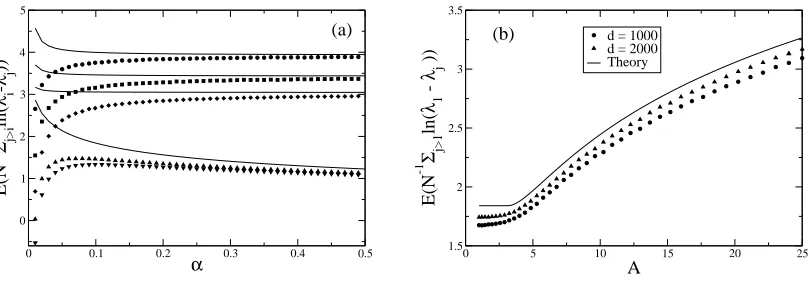
of the replica trick (see Appendix A). Specifically we have forα>A−_i 2,

lim

N,d→∞N −1_E

ξ

∑

j>k

ln(λi−λj)

!

= lnσ2 ₋ (α−1₋1)ln(1+Ai) +α−1ln Ai +

1

αAi

, (18)

whilst forα<A−_i 2we have,

lim

N,d→∞N −1_E

ξ

∑

j>k

ln(λi−λj)

!

= lnσ2 ₋ (α−1₋1)ln(1+α−12) + α−1lnα− 1

2 + α−

1

2 . (19)

The asymptotic behaviour of the ratio Area(Vk(Rd−N+1))/Area(Vk(Rd))is easily evaluated to give,

ln

Area(Vk(Rd−N+1))

Area(Vk(Rd))

= Nk

2

−lnπ + lnd

2 − (α

−1

−1)ln(1₋α) ₋1

+O(ln N). (20)

Substituting Equations (18),(19),(20) and the asymptotic values for ˆv and ˆliinto Equation (16), we

obtain after some straight-forward algebra,

Eξ(ln p(D|k)) =

N

2

k

∑

i=1

Θ(α−A−_i 2)

Ai−

1 αAi

+ (α−1−1)ln

1+Ai

1+ (1/αAi)

+α−1ln

1 αA2_i

− Nd₂ lnσ2 ₋ Nd

2 +O(ln N). (21)

If we set x=α−1_{we can write the summand in Equation (21) as}Θ₍α_−A−2

i )f(x,Ai)where,

f(x,A) =A+ x ln x + (x₋1)ln(1+A) ₋ 2x ln A ₋(x₋1)ln(1+xA−1) ₋ xA−1.

We find that,

f(A2,A) = 0 , ∂f

∂x

x=A2

= 0 , ∂ 2_f

∂x2 > 0 for x < A 2_,

ithprincipal component results in an increase in the asymptotic approximation to the log-evidence. Conversely ifα<A−_i 2there is no change in the asymptotic approximation to the log-evidence on including the ithprincipal component. This is a satisfying result since we have already commented in Section 3 that forα<A−_i 2the sample covariance eigenspectrum is asymptotically indistinguish-able from that produced from a population model with Ai≡0, and so therefore from a Bayesian

model selection perspective all population models with Ai<α−

1

2 are equally likely (provide an

equally accurate description of the observed data). Ultimately this is due to the fact that we are considering models with a finite number, k, of signal components, and so in the asymptotic limit we are considering a vanishingly small proportion of sample covariance eigenvalues as representing signal components. With the non-zero sample covariance eigenvalues giving a dense covering of the range[λmin,λmax]in the asymptotic limit, the largest few sample covariance eigenvalues, which

are not distinct from the Marˇcenko-Pastur bulk distribution given in Equation (2) will be aggregated at the upper edge of the bulk, where they do not lead to any change in the log-evidence. For finite sample sizes we would expect the higher order terms in the expansion of the log-evidence to lead to a decrease in the log-evidence on inclusion of principal components that correspond to sample covariance eigenvalues that are below the bulk edge. However, in the asymptotic limit we can ap-ply an Occam’s Razor like argument and only select those principal components that increase the log-evidence. The limiting model selection estimate, ˆS, for the true signal dimensionality, S, then simply corresponds to counting the number of sample covariance eigenvalues that are beyond the upper edge of the Marˇcenko-Pastur bulk distribution. That is,

ˆ

S =

d

∑

j=1

Θ(λj − λmax).

The asymptotic analysis of the “overlap” method reveals that unbiased estimates of the pop-ulation signal eigenvalues can be recovered and that, asymptotically, model selection based upon the “overlap” approximation to the log-evidence performs optimally. From Fig.2b it would ap-pear that, at least for larger values ofα, model selection based upon Minka’s approximation to the log-evidence also approaches 100% accuracy as d_→∞. Is it possible that the two different approx-imations to the log-evidence asymptotically have the same model selection performance? Starting from Minka’s approximation to the Bayesian evidence p(D_|k)given in Equation (7) we have,

ln p(D_|k) _{' −}ln Area(Vk(Rd))−

N 2

k

∑

i=1

lnλi −

N

2(d−k)ln ˆv +

m+k

2 ln 2π

−1

2

k

∑

i=1

d

∑

j=i+1

h ln(_Λˆ−1

j −Λˆ−i 1) + ln(λi−λj) + ln N

i

− k

2ln N, (22)

where ˆΛi =Nλi/(N−1) for i≤k and ˆΛi =v for iˆ >k, with ˆv defined in Equation (6). In this

instance O(N−1_{) contributions to E}

ξ(v)ˆ do make a contribution to the leading order asymptotic

term in Eξ(ln p(D|k)). From the definition of the point estimate ˆv in (6) we find,

Eξ(v) = (1ˆ +N−1(kα−1))Eξ(d−1tr ˆC) −

α

N

k

∑

j=1

Eξ(λj) + O(N−2).

Eξ(v) =ˆ σ2 +

ασ2

N

S

∑

j=1

Aj +

σ2

N(kα−1)

−ασ

2

N

k

∑

i=1

h

Θ(α₋A−_i 2)(1+Ai)(1+ (1/αAi)) +Θ(A−i 2−α)(1+α−

1 2)2

i

+O(N−2).

Retaining only k-dependent terms, the leading order asymptotic contribution to Eξ(ln p(D|k))can

be obtained within this approximation as,

Eξ(ln p(D|k)) =

N 2

k

∑

i=1

h

Θ(α₋A−_i 2)fM(x,Ai) + Θ(A−i 2−α)fM(x,α−

1 2)

i

+O(ln N),

where the subscript M on the function fM(x,A)is used to denote the asymptotic incremental change

to the log-evidence obtained from Minka’s approximation given in Equation (22), and again x=

α−1_{. Specifically f}

M(x,A)is given as,

fM(x,A) =A+ x ln x + (x−1)ln(1+A) − 2x ln A −x ln

1+xA−1+xA−2. (23) The transition point at which a signal component is strong enough to be distinguishable from the Marˇcenko-Pastur bulk distribution in Equation (2) is given by a signal strength A=α−1

2. If we put

A=yα−12 =y√x, then y directly measures the signal strength relative to that at which it is first

detectable. We can then write Equation (23) as,

fM(x,A=y√x) = (x−1)ln(1+y√x) −x ln 1+y√x+y2

+y√x.

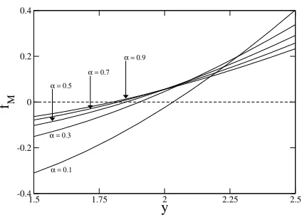
A plot of fM(x=α−1,A=yα−

1

2)against y for different fixed values ofαis shown in Figure 4. From Fig.4 we can see that at the transition point, y=1, fMis negative, and so selection of the ithprincipal

component will result in a reduction of the log-evidence, even if the signal strength Aiis sufficiently

strong enough for the ithsample covariance eigenvalue to be distinct from the Marˇcenko-Pastur bulk distribution. Thus, even though a detectable signal is present model selection based upon Equation (22) would not include that signal component. For the largest value ofαshown fMdoes not become

positive until approximately y>1.8. Therefore, even forα=0.9, not until the signal strength Aiis

1.8 times stronger than it need be for detection will the ith signal component be correctly selected whilst using Minka’s approximation to the log-evidence in Equation (22). For smaller values ofα even stronger signal strengths are required, for example, y>2.0 atα=0.1. For the simulations results shown in Fig.2b it is only at the largest value ofαshown that we have fM>0 for all three

signal components, and thus that all three signal components are guaranteed to be detectable in the asymptotic limit.

6. Comparison with Frequentist Approaches

1.5 1.75 2 2.25 2.5 y

-0.4 -0.2 0 0.2 0.4

f M

α = 0.1 α = 0.3 α = 0.5

α = 0.7 α = 0.9

Figure 4: Plot of the function fM(x=α−1,A=yα−

1

2)against y for different values ofα. N f_M/2 represents the incremental change (to leading order) in the log-evidence on retaining a principal component corresponding to a signal component of strength A=yα−12. The horizontal dashed line denotes the zero level for fM.

the upper spectral edge,λmax=σ2(1+α−

1

2)2, of the bulk eigenvalue distribution. Whilst this result appears intuitive from the viewpoint of the behaviour of eigenspectra of large sample covariance matrices presented in Section 3, we have also shown that not all approximations to the Bayesian ev-idence reduce in the asymptotic limit to this optimal choice for model selection. How then does the “overlap” method for model selection compare to other approaches, for example more traditional non-Bayesian approaches for dimensionality selection in PCA? In the asymptotic limit N_→∞, where we have an infinite amount of data, we would naively expect frequentist and correctly formu-lated Bayesian approaches to model selection to give similar answers.

One of the most commonly applied techniques for dimensionality selection for PCA is to select sample covariance eigenvalues (and corresponding eigenvectors) that account for a fixed percentage of the total variance, for example, 90%. Typically this may only be the top two or three eigenvalues. Alternative methods consist of producing a ‘scree plot’, that is, plot of eigenvalue against rank, and attempting to detect by eye an ‘elbow’ in the plot where there is a significant change in scale of the sample covariance eigenvalues, supposedly reflecting the change from signal dominated eigenvalues to noise dominated eigenvalues. However, with sample covariance eigenvalues potentially being highly biased even when the population covariance is isotropic this is not always a reliable or easily implemented technique.

Hypothesis tests have been developed to detect departure from sphericity of the population co-variance, based upon using tr ˆC as the test statistic (John, 1971; Nagao, 1973). This approach has been modified by Ledoit and Wolf (2002) to account for smaller sample sizes but is still essentially only appropriate forα>1. The effect of smaller values ofαcan be accounted for since the asymp-totic form of the expected spectrum is given by the Marˇcenko-Pastur distribution (2) whenC=σ2_I.

the 45 degree line in these Wachter plots indicate potentially signal containing principal compo-nents. At finite values of d a more principled, but non-Bayesian, approach would be to perform a series of iterative hypothesis tests whereby the null-hypothesis H0 is that of a model containing k

signal components. Comparison of the(k+1)th _{sample covariance eigenvalue,} λ

k+1, against the

sampling distribution ofλk+1 under H0 would allow for potential rejection of the null-hypothesis

and inclusion of the(k+1)th_{principal component as representing genuine signal in the data. After}

setting a rate at which one wishes to control the Type-I error, for example,γ=0.05, testing of the (k+1)th_,(k+2)th_{, . . .principal components proceed via,}

H0 : C≡σˆ2I , σˆ2 = d−1∑dj=1λj , k=0

while p(λ>λk+1|k,d,N)<γ

k→k+1

ˆ

Λk = λk

ˆ

σ2 _{= (d−k)}−1_∑d j=k+1λj

H0 : C≡diag(Λˆ1, . . . ,Λˆk,σˆ2, . . . ,σˆ2)

end while

To implement this testing procedure we need the cumulative sampling distribution p(λ>λk+1|k,d,N)

of the(k+1)th _{sample covariance eigenvalue under the null hypothesis ofC containing k signal}

components - that is the probability, when the population covariance contains only k signal compo-nents, of the(k+1)th_{sample covariance eigenvalue being larger than the eigenvalueλ}

k+1observed

in the real sample data. Johnstone (2001) has derived the sampling distribution for k=0 by ex-tending the analysis of Tracy and Widom (1996) on the Gaussian Orthogonal Ensemble (GOE) of random matrices. We can define location and scale constants,

µNd = N−1

√

N₋1 + √d2 ,

and

σNd = N−1

√

N₋1 + √d

1

√

N₋1 +

1

√

d 1₃

.

Then for data drawn from an isotropic population covariance, C = σ2_{I, the largest sample}

co-variance eigenvalueλ1(suitably centred and scaled) converges in distribution to the Tracy-Widom

distribution W1. Specifically one has,

(λ1/σ2)−µNd

σNd

D

→W1∼F1,

where,

F1(s) = exp

−1₂

Z ∞ s

q(x) + (x₋s)q2(x)dx

,

with q(x)being the solution to the Painlev´e II differential equation that is asymptotically equivalent to the Airy function Ai(x),

d2q(x)

dx2 = xq(x) +2q

3_(x),

200 400 600 800 1000

Dimension d

0 0.2 0.4 0.6 0.8 1

Probability Correct

(a)

N = 100 N = 200 N = 400

200 400 600 800 1000

Dimension d

0 0.2 0.4 0.6 0.8 1

Probability Correct

(b)

α = 0.2 α = 0.3 α = 0.4

Figure 5: Comparison of the model selection accuracy for the “overlap” method (solid black sym-bols) with a null hypothesis test based upon the Tracy-Widom distribution for the largest eigenvalue of a sample covariance matrix (open symbols). a)Plot of model selection ac-curacy against data dimension d at fixed values of N. (b)Plot of model selection acac-curacy against data dimension for fixed values ofα.

Note that the centering constant µNd→λmax, up to an irrelevant factor ofσ2. That is, the edge of the

Marˇcenko-Pastur distribution, as N,d_→∞at fixed α. More recent analysis of the distribution of

λ1when the data is complex and contains signal has been performed by Baik et al. (2005). The

au-thors provide conjectures for the behaviour of the sampling distribution ofλ1when the data is real,

based upon their analysis of the complex case, but this still does not provide a means of calculating the sampling distribution p(λk+1|k,d,N)for k>0. Instead Johnstone (2001) derives the inequality

p(λ>λk+1|k,d,N)<p(λ>λ1|0,d−k,N), with the latter distribution being given in terms of the

Tracy-Widom distribution. Consequently, at finite N this provides a conservative hypothesis test since use of p(λ1|0,d−k,N) yields an over-estimate of the tail area of the sampling distribution

p(λk+1|k,d,N), and therefore an over-estimate of the Type-I error rate. With the varianceσ2_Nd

tend-ing to zero as N_→∞, then in the asymptotic limit N_→∞the series of hypothesis tests given above corresponds simply to determining how many sample covariance eigenvaluesλiare aboveλmax- the

edge of the Marˇcenko-Pastur bulk distribution - and so, as naively expected, is in agreement with the behaviour of the “overlap” method in the distinguished asymptotic limit.

and Figure 3. We have controlled the Type-I error at the 5% level (γ=0.05) with the value of the abscissa for the 95thcentile of the Tracy-Widom distribution taken from Johnstone (2001). Within Fig.5(b) we would expect all model selection accuracies to converge to 1 as d,N_→∞since all the signal strengths have been chosen to be above their respective retarded learning transition points and therefore the sample eigenvalues corresponding to signal directions are all distinguishable from the Marˇcenko-Pastur bulk in this limit. However, for finite d and N Fig.5(a) and (b) reveal that overall the hypothesis testing approach has a superior model selection accuracy when both N andα are relatively small. By definition, the hypothesis test only considers a sample covariance eigenvalue to represent a signal if it exceeds that expected from the null model by more than reasonable sam-pling variation. As samsam-pling variation will be greater at smaller values of N we might expect the hypothesis testing approach to be more sensitive for model selection than the “overlap” approach within this regime, particularly since higher order terms in the asymptotic expansion of the Bayesian evidence, that have not been incorporated into the “overlap” evidence approximation, will be more significant for smaller values of d and N. For larger values of d and N, the conservative nature of any hypothesis testing approach may adversely affect its model selection accuracy in comparison to a Bayesian evidence based approach.

7. Discussion & Conclusions

For calculations within high-dimensional inference problems we have argued that, rather than using results obtained by considering the traditional large sample limit N_→∞, better approximations may be obtained by considering them to be close to the asymptotic value obtained in some distinguished limit, even though the sample size N may naively be considered large enough for routine application of the Laplace approximation to be accurate. What constitutes a large sample size, N, should clearly be defined with respect to the data dimensionality d. For PCA the appropriate distinguished asymp-totic limit is d,N_→∞, withα=N/d fixed, though for other models different distinguished limits may need to be considered in order to observe meaningful non-trivial behaviour that is distinct from the large sample limit, N_→∞. For example, statistical physics studies of independent component analysis (ICA) suggests that d_→∞with N=αd32 at fixedαwould be the appropriate distinguished limit to consider (Urbanczik, 2003). However, irrespective of the particular distinguished limit con-sidered when developing an asymptotic approximation, one needs to be careful to keep track of the increasing number of contributions as d_→∞, and potentially large contributions resulting from the rotational degeneracy of the integrand in the formulation of the Bayesian evidence.

potentially superior estimation schemes, based upon a Gaussian parametrization of the integrand, that perform well when the integrand is essentially unimodal, for example expectation propagation based schemes (Minka, 2001b) or variational approximation similar to that employed by Bishop (1999b) for model selection within Bayesian PCA, although it should be noted that Bishop (1999b) does not impose an orthogonal constraint upon the low dimensional decomposition of the popula-tion covariance. However, it is the fact that one has to reformulate the evidence calculapopula-tion for a Gaussian approximation to be accurate that is our main finding here, not the particular choice of approximation scheme that one employs once the reformulation has been made. Of greater interest perhaps is the fact that we have been able to demonstrate the asymptotic equivalence of the Bayesian evidence based model selection criterion and the frequentist hypothesis testing approach to model selection. Furthermore, analysis of the asymptotic behaviour of the “overlap” approximation to the log-evidence reveals that the estimators of the population signal eigenvalues are unbiased, at least for the “spiked” covariance models considered here.

The influence of high data dimensionality on estimates of model parameters can be explicitly demonstrated by re-visiting Minka’s original Laplace approximation to the evidence. Although Minka’s derivation provides a poorer approximation to the model evidence, in the distinguished limit N,d _→∞ at fixed α, in comparison to the “overlap” approximation, it is still the correct leading order approximation in the asymptotic limit N_→∞at arbitrary fixed values of d. Therefore it contains information about how the model evidence behaves for large values of N and d. This suggests that Minka’s Laplace approximation to the model evidence could be re-used to develop improved point estimates of population covariance eigenvalues_{Λi}. One proceeds by noting that

the eigenvectors of ˆC are the maximum posterior estimates ofU for arbitrary choices of_{li}and

v, since projection of the sample data onto the sample covariance eigenvectors retains the greatest variance. We can simply re-use Minka’s approach to perform the Gaussian integration overU about this maximum posterior point, yielding p(D_|{li},v)which can then be optimized with respect to{li}

and v. Specifically we have the following approximation to the log-evidence (takingη_→0),

−N+1

2

k

∑

i=1

ln li + (d−k)ln v

!

− N

2v

N−1

∑

j=1 λj +

N 2

k

∑

i=1

(v−1_−l−1

i )λi

− 1₂ln_|AZ| +ln

N

m+k

2 ln 2π − k

2ln N, (24)

ln_|AZ| = m ln N +

k

∑

i=1

(d₋k)ln(v−1₋l_i−1) +

k

∑

j=i+1

ln(l−_j 1₋l_i−1) +

d

∑

j=i+1

ln(λi−λj)

!

.

It should be noted that the contribution from ln_|AZ| is extensive in d and therefore affects the

construction of point estimates for_{li}and v. Retaining only extensive terms in Equation (24) and

locating stationary points with respect to li and v yields estimators ˆli,v. In the asymptotic limitˆ

N_→∞these estimators are given by,

0 = vˆ−1ˆl_i2 ₋ ˆli(1+vˆ−1λi−α−1) +λi,

ˆ

v = d−1

N−1

∑