Maximum Entropy Discrimination Markov Networks
Jun Zhu [email protected]
Eric P. Xing [email protected]
Machine Learning Department Carnegie Mellon University
5000 Forbes Avenue, Pittsburgh, PA 15213
Editor: Michael Collins
Abstract
The standard maximum margin approach for structured prediction lacks a straightforward proba-bilistic interpretation of the learning scheme and the prediction rule. Therefore its unique advan-tages such as dual sparseness and kernel tricks cannot be easily conjoined with the merits of a probabilistic model such as Bayesian regularization, model averaging, and ability to model hidden variables. In this paper, we present a new general framework called maximum entropy discrimina-tion Markov networks (MaxEnDNet, or simply, MEDN), which integrates these two approaches and combines and extends their merits. Major innovations of this approach include: 1) It extends the conventional entropy discrimination learning of classification rules to a new structural max-entropy discrimination paradigm of learning a distribution of Markov networks. 2) It generalizes the extant Markov network structured-prediction rule based on a point estimator of model coeffi-cients to an averaging model akin to a Bayesian predictor that integrates over a learned posterior distribution of model coefficients. 3) It admits flexible entropic regularization of the model during learning. By plugging in different prior distributions of the model coefficients, it subsumes the well-known maximum margin Markov networks (M3N) as a special case, and leads to a model similar to an L1-regularized M3N that is simultaneously primal and dual sparse, or other new types of Markov networks. 4) It applies a modular learning algorithm that combines existing variational inference techniques and convex-optimization based M3N solvers as subroutines. Essentially, MEDN can be understood as a jointly maximum likelihood and maximum margin estimate of Markov network. It represents the first successful attempt to combine maximum entropy learning (a dual form of maximum likelihood learning) with maximum margin learning of Markov network for structured input/output problems; and the basic principle can be generalized to learning arbitrary graphical models, such as the generative Bayesian networks or models with structured hidden variables. We discuss a number of theoretical properties of this approach, and show that empirically it outper-forms a wide array of competing methods for structured input/output learning on both synthetic and real OCR and web data extraction data sets.
Keywords: maximum entropy discrimination, structured input/output model, maximum margin
Markov network, graphical models, entropic regularization, L1regularization
1. Introduction
that explicitly exploit the structured dependencies among input elements and structured interpreta-tional outputs. Major instances of such models include the condiinterpreta-tional random fields (CRFs) (Laf-ferty et al., 2001), Markov networks (MNs) (Taskar et al., 2003), and other specialized graphical models (Altun et al., 2003). Various paradigms for training such models based on different loss func-tions have been explored, including the maximum conditional likelihood learning (Lafferty et al., 2001) and the maximum margin learning (Altun et al., 2003; Taskar et al., 2003; Tsochantaridis et al., 2004), with remarkable success.
The likelihood-based models for structured predictions are usually based on a joint distribution of both input and output variables (Rabiner, 1989) or a conditional distribution of the output given the input (Lafferty et al., 2001). Therefore this paradigm offers a flexible probabilistic framework that can naturally facilitate: hidden variables that capture latent semantics such as a generative hier-archy (Quattoni et al., 2004; Zhu et al., 2008a); Bayesian regularization that imposes desirable biases such as sparseness (Lee et al., 2006; Wainwright et al., 2006; Andrew and Gao, 2007); and Bayesian prediction based on combining predictions across all values of model parameters (i.e., model av-eraging), which can reduce the risk of overfitting. On the other hand, the margin-based structured prediction models leverage the maximum margin principle and convex optimization formulation un-derlying the support vector machines, and concentrate directly on the input-output mapping (Taskar et al., 2003; Altun et al., 2003; Tsochantaridis et al., 2004). In principle, this approach can lead to a robust decision boundary due to the dual sparseness (i.e., depending on only a few support vectors) and global optimality of the learned model. However, although arguably a more desirable paradigm for training highly discriminative structured prediction models in a number of application contexts, the lack of a straightforward probabilistic interpretation of the maximum-margin models makes them unable to offer the same flexibilities of likelihood-based models discussed above.
For example, for domains with complex feature space, it is often desirable to pursue a “sparse” representation of the model that leaves out irrelevant features. In likelihood-based estimation, sparse model fitting has been extensively studied. A commonly used strategy is to add an L1-penalty to the
likelihood function, which can also be viewed as a MAP estimation under a Laplace prior. However, little progress has been made so far on learning sparse MNs or log-linear models in general based on the maximum margin principle. While sparsity has been pursued in maximum margin learning of certain discriminative models such as SVM that are “unstructured” (i.e., with a univariate output), by using L1-regularization (Bennett and Mangasarian, 1992) or by adding a cardinality constraint (Chan
et al., 2007), generalization of these techniques to structured output space turns out to be non-trivial, as we discuss later in this paper. There is also very little theoretical analysis on the performance guarantee of margin-based models under direct L1-regularization. Our empirical results as shown in
this paper suggest that an L1-regularized maximum margin Markov network, even when estimable,
can be sensitive to the magnitude of the regularization coefficient. Discarding the features that are not completely irrelevant can potentially hurt generalization ability. Another example, it is well known that presence of hidden variables in MNs can cause significant difficulty for maximum margin learning. Indeed, semi-supervised or unsupervised learning of structured maximum margin model remains an open problem of which progress was only made in a few special cases, with usually computationally very expensive algorithms (Xu et al., 2006; Altun et al., 2006; Brefeld and Scheffer, 2006).
the Bayesian regularization techniques for learning structured prediction models. It integrates the spirit of maximum margin learning from SVM, the design of discriminative structured prediction model in maximum margin Markov networks (M3N), and the ideas of entropic regularization and model averaging in maximum entropy discrimination methods (Jaakkola et al., 1999). Essentially, MaxEnDNet can be understood as a jointly maximum likelihood and maximum margin estimate of Markov networks. It allows one to learn a distribution of structured prediction models that offers a wide range of important advantages over conventional models such as M3N, including more
ro-bust prediction due to an averaging prediction-function based on the learned distribution of models, Bayesian-style regularization that can lead to a model that is simultaneous primal and dual sparse, and allowance of hidden variables and semi-supervised learning based on partially labeled data.
While the formalism of MaxEnDNet is extremely general, our main focus and contributions of this paper will be concentrated on the following results. We will formally define the MaxEnD-Net as solving a generalized entropy optimization problem subject to expected margin constraints on the structured predictions, and under an arbitrary prior of feature coefficients; and we derive a general form of the solution to this problem. An interesting insight immediately following this general form is that, a trivial assumption on the prior distribution of the coefficients, that is, a stan-dard normal, reduces the linear MaxEnDNet to the stanstan-dard M3N, as shown in Theorem 3. This understanding opens the way to use different priors for MaxEnDNet to achieve more interesting regularization effects. We show that, by using a Laplace prior for the feature coefficients, the re-sulting Laplace MaxEnDNet (LapMEDN) is effectively an M3N that is not only dual sparse (i.e., defined by a few support vectors), but also primal sparse (i.e., shrinkage on coefficients correspond-ing to irrelevant features). We develop a novel variational learncorrespond-ing method for the LapMEDN, which leverages on the hierarchical/scale-mixture representation of the Laplace prior (Andrews and Mallows, 1974; Figueiredo, 2003) and the reducibility of MaxEnDNet to M3N, and combines the variational Bayesian technique with existing convex optimization algorithms developed for M3N (Taskar et al., 2003; Bartlett et al., 2004; Ratliff et al., 2007). We also provide a formal analysis of the generalization error of the MaxEnDNet, and prove a PAC-Bayes bound on the prediction error by MaxEnDNet. We performed a thorough comparison of the Laplace MaxEnDNet with com-peting methods, including M3N (i.e., the Gaussian MaxEnDNet), L1-regularized M3N (Zhu et al.,
2009b), CRFs, L1-regularized CRFs, and L2-regularized CRFs, on both synthetic and real structured
input/output data. The Laplace MaxEnDNet exhibits mostly superior, and sometimes comparable performance in all scenarios been tested.
As demonstrated in our recent work (Zhu et al., 2008c, 2009a), MaxEnDNet is not limited to fully observable MNs, but can readily facilitate jointly maximum entropy and maximum margin learning of partially observed structured I/O models, and directed graphical models such as the supervised latent Dirichlet allocation (LDA). Due to space limit, we leave these instantiations and generalizations to future papers.
Then, we show empirical results on both synthetic and real OCR and web data extraction data sets in Section 7. Section 8 discusses some related work and Section 9 concludes this paper.
2. Preliminaries
In structured prediction problems such as natural language parsing, image annotation, or DNA decoding, one aims to learn a function h :
X
→Y
that maps a structured input x∈X
, e.g., a sentence or an image, to a structured output y∈Y
, e.g., a sentence parsing or a scene annotation, where, unlike a standard classification problem, y is a multivariate prediction consisting of multiple labeling elements. Let L denote the cardinality of the output, and ml where l=1, . . . ,L denote the arity ofeach element, then
Y
=Y
1× ··· ×Y
LwithY
l ={a1, . . . ,aml}represents a combinatorial space of structured interpretations of the multi-facet objects in the inputs. For example,Y
could correspond to the space of all possible instantiations of the parse trees of a sentence, or the space of all possible ways of labeling entities over some segmentation of an image. The prediction y≡(y1, . . . ,yL) isstructured because each individual label yl∈
Y
lwithin y must be determined in the context of otherlabels yl′6=l, rather than independently as in classification, in order to arrive at a globally satisfactory
and consistent prediction.
Let F :
X
×Y
→Rrepresent a discriminant function over the input-output pairs from which one can define the predictive function, and letH
denote the space of all possible F. A common choice of F is a linear model, F(x,y; w) =g(w⊤f(x,y)), where f= [f1. . .fK]⊤ is a K-dimensionalcolumn vector of the feature functions fk:
X
×Y
→R, and w= [w1. . .wK]⊤is the correspondingvector of the weights of the feature functions. Typically, a structured prediction model chooses an optimal estimate w⋆ by minimizing some loss function J(w), and defines a predictive function in terms of an optimization problem that maximizes F(·; w⋆)over the response variable y given an input x:
h0(x; w⋆) =arg max
y∈Y(x)F(x,y; w
⋆), (1)
where
Y
(x)⊆Y
is the feasible subset of structured labels for the input x. Here, we assume thatY
(x)is finite for any x.Depending on the specific choice of g(·)(e.g., linear, or log linear), and the loss function J(w) (e.g., likelihood, or margin-based loss) for estimating the parameter w⋆, incarnations of the general structured prediction formalism described above can be seen in classical generative models such as the HMM (Rabiner, 1989) where g(·)can be an exponential family distribution function and J(w) is the (negative) joint likelihood of the input and its labeling; and in recent discriminative models such as CRFs (Lafferty et al., 2001), where g(·)is a Boltzmann machine and J(w)is the (negative) conditional likelihood of the structured labeling given input; and the M3N (Taskar et al., 2003), where g(·)is an identity function and J(w)is a loss defined on the margin between the true labeling and any other feasible labeling in
Y
(x). Our approach toward a more general discriminative training is based on a maximum entropy principle that allows an elegant combination of the discriminative maximum margin learning with the generative Bayesian regularization and hierarchical modeling, and we consider the more general problem of finding a distribution of F(·; w)overH
that enables a convex combination of discriminant functions for robust structured prediction.framework, given a set of fully observed training data
D
={hxi,yii}Ni=1, we obtain a point estimate
of the weight vector w by solving the following max-margin problem P0 (Taskar et al., 2003):
P0(M3N): min w,ξ
1 2kwk
2+C
∑
N i=1ξi
s.t.∀i,∀y=6 yi: w⊤∆fi(y)≥∆ℓi(y)−ξi,ξi≥0,
where∆fi(y) =f(xi,yi)−f(xi,y)and∆Fi(y; w) =w⊤∆fi(y)is the “margin” between the true label
yi and a prediction y,∆ℓi(y)is a labeling loss with respect to yi, andξi represents a slack variable
that absorbs errors in the training data. Various forms of the labeling loss have been proposed in the literature (Tsochantaridis et al., 2004). In this paper, we adopt the hamming loss used by Taskar et al. (2003): ∆ℓi(y) =∑Lj=1I(yj6=yij), whereI(·)is an indicator function that equals to one if the
argument is true and zero otherwise. The problem P0 is not directly solvable by using a standard constrained optimization toolbox because the feasible space for w,
F
0= nw : w⊤∆fi(y)≥∆ℓi(y)−ξi;∀i,∀y6=yi o
,
is defined by O(N|
Y
|) number of constraints, andY
is exponential to the size of the input x. Exploring sparse dependencies among individual labels yl in y, as reflected in the specific design ofthe feature functions (e.g., based on pair-wise labeling potentials in a pair-wise Markov network), and the convex duality of the objective, efficient optimization algorithms based on cutting-plane (Tsochantaridis et al., 2004) or message-passing (Taskar et al., 2003) have been proposed to obtain an approximate optimum solution to P0. As described shortly, these algorithms can be directly employed as subroutines in solving our proposed model.
3. Maximum Entropy Discrimination Markov Networks
Instead of learning a point estimator of w as in M3N, in this paper, we take a Bayesian-style ap-proach and learn a distribution p(w), in a max-margin manner. For prediction, we employ a convex combination of all possible models F(·; w)∈
H
based on p(w), that is:h1(x) =arg max
y∈Y(x)
Z
p(w)F(x,y; w)dw. (2)
based on the Bayes theorem, but a maximum entropy principle that biases towards a distribution that makes less additional assumptions over a given prior over the predictive models. We emphasize that this “posterior” is different from, and should not be confused with, the conventional Bayesian posterior defined according to the Bayes rule.
It is well-known that exponential family distributions can be expressed variationally as the so-lution to a maximum entropy estimation subject to moment constraints, and the maximum entropy estimation of parameters can be understood as a dual to the maximum likelihood estimation of the parameters of exponential family distributions. Thus our combination of the maximum entropy principle with the maximum margin principle to be presented in the sequel offers an elegant way of achieving jointly maximum margin and maximum likelihood effects on learning structured in-put/output Markov networks, and in fact, general exponential family graphical models.
3.1 Structured Maximum Entropy Discrimination
Given a training set
D
of structured input-output pairs, analogous to the feasible spaceF
0 for theweight vector w in a standard M3N (c.f., problem P0), we define the feasible subspace
F
1 for the weight distribution p(w)by a set of expected margin constraints:F
1=np(w): Zp(w)[∆Fi(y; w)−∆ℓi(y)]dw≥ −ξi,∀i,∀y6=yi o
.
We learn the optimum p(w) from
F
1 based on a structured maximum entropy discriminationprinciple generalized from the maximum entropy discrimination (Jaakkola et al., 1999). Under this principle, the optimum p(w)corresponds to the distribution that minimizes its relative entropy with respect to some chosen prior p0, as measured by the Kullback-Leibler divergence between p and p0:
KL(p||p0) =hlog(p/p0)ip, whereh·ipdenotes the expectations with respect to p. If p0is uniform,
then minimizing this KL-divergence is equivalent to maximizing the entropy H(p) =−hlog pip. A
natural information theoretic interpretation of this formulation is that we favor a distribution over the discriminant function class
H
that bears minimum assumptions among all feasible distributions inF
1. The p0is a regularizer that introduces an appropriate bias, if necessary.To accommodate non-separable cases in the discriminative prediction problem, instead of min-imizing the usual KL, we optimize the generalized entropy (Dud´ık et al., 2007; Lebanon and Laf-ferty, 2001), or a regularized KL-divergence, KL(p(w)||p0(w)) +U(ξ), where U(ξ) is a closed
proper convex function over the slack variables. This term can be understood as an additional “po-tential” in the maximum entropy principle. Putting everything together, we can now state a general formalism based on the following maximum entropy discrimination Markov network framework:
Definition 1 (Maximum Entropy Discrimination Markov Networks) Given training data
D
={hxi,yii}Ni=1, a chosen form of discriminant function F(x,y; w), a loss function∆ℓ(y), and an ensu-ing feasible subspace
F
1 (defined above) for parameter distribution p(w), the MaxEnDNet model that leads to a prediction function of the form of Equation (2) is defined by the following generalized relative entropy minimization with respect to a parameter prior p0(w):P1(MaxEnDNet): min
p(w),ξKL(p(w)||p0(w)) +U(ξ)
The P1 defined above is a variational optimization problem over p(w)in a subspace of valid parameter distributions. Since both the KL and the function U in P1 are convex, and the constraints in
F
1are linear, P1 is a convex program. In addition, the expectationshF(x,y; w)ip(w)are requiredto be bounded in order for F to be a meaningful model. Thus, the problem P1 satisfies the Slater’s condition1 (Boyd and Vandenberghe, 2004, chap. 5), which together with the convexity make P1 enjoy nice properties, such as strong duality and the existence of solutions. The problem P1 can be solved via applying the calculus of variations to the Lagrangian to obtain a variational extremum, followed by a dual transformation of P1. We state the main results below as a theorem, followed by a brief proof that lends many insights into the solution to P1 which we will explore in subsequent analysis.
Theorem 2 (Solution to MaxEnDNet) The variational optimization problem P1 underlying the
MaxEnDNet gives rise to the following optimum distribution of Markov network parameters w:
p(w) = 1
Z(α)p0(w)exp
n
∑
i,y6=yi
αi(y)[∆Fi(y; w)−∆ℓi(y)] o
, (3)
where Z(α) is a normalization factor and the Lagrange multipliers αi(y) (corresponding to the
constraints in
F
1) can be obtained by solving the dual problem of P1:D1 : max
α −log Z(α)−U
⋆(α)
s.t. αi(y)≥0,∀i,∀y6=yi
where U⋆(·) is the conjugate of the slack function U(·), that is, U⋆(α) =supξ(∑i,y6=yiαi(y)ξi− U(ξ)).
Proof (sketch) Since the problem P1 is a convex program and satisfies the Slater’s condition, we
can form a Lagrangian function, whose saddle point gives the optimal solution of P1 and D1, by introducing a non-negative dual variableαi(y) for each constraint in
F
1 and another non-negativedual variable c for the normalization constraintR
p(w)dw =1. Details are deferred to Appendix B.1.
Since the problem P1 is a convex program and satisfies the Slater’s condition, the saddle point of the Lagrangian function is the KKT point of P1. From the KKT conditions (Boyd and Vanden-berghe, 2004, Chap. 5), it can be shown that the above solution enjoys dual sparsity, that is, only a few Lagrange multipliers will be non-zero, which correspond to the active constraints whose equal-ity holds, analogous to the support vectors in SVM. Thus MaxEnDNet enjoys a similar generaliza-tion property as the M3N and SVM due to the the small “effective size” of the margin constraints. But it is important to realize that this does not mean that the learned model is “primal-sparse”, that is, only a few elements in the weight vector w are non-zero. We will return to this point in Section 4. For a closed proper convex functionφ(µ), its conjugate is defined asφ⋆(ν) =supµ[ν⊤µ−φ(µ)].
In the problem D1, by convex duality (Boyd and Vandenberghe, 2004), the log normalizer log Z(α) can be shown to be the conjugate of the KL-divergence. If the slack function is U(ξ) =Ckξk=
1. SincehF(x,y; w)ip(w) are bounded andξi≥0, there always exists a ξ, which is large enough to make the pair
C∑iξi, it is easy to show that U⋆(α) =I∞(∑yαi(y)≤C, ∀i), whereI∞(·)is a function that equals
to zero when its argument holds true and infinity otherwise. Here, the inequality corresponds to the trivial solutionξ=0, that is, the training data are perfectly separable. Ignoring this inequality does not affect the solution since the special caseξ=0 is still included. Thus, the Lagrange multipliers αi(y) in the dual problem D1 comply with the set of constraints that∑yαi(y) =C, ∀i. Another
example is U(ξ) =KL(p(ξ)||p0(ξ))by introducing uncertainty on the slack variables (Jaakkola
et al., 1999). In this case, expectations with respect to p(ξ) are taken on both sides of all the constraints in
F
1. Take the duality, and the dual function of U is another log normalizer. Moredetails were provided by Jaakkola et al. (1999). Some other U functions and their dual functions are studied by Lebanon and Lafferty (2001) and Dud´ık et al. (2007).
Unlike most extant structured discriminative models including the highly successful M3N, which rely on a point estimator of the parameters, the MaxEnDNet model derived above gives an optimum parameter distribution, which is used to make prediction via the rule (2). Indeed, as we will show shortly, the MaxEnDNet is strictly more general than the M3N and subsumes the later as a special case. But more importantly, the MaxEnDNet in its full generality offers a number of important advantages while retaining all the merits of the M3N. First, MaxEnDNet admits a prior that can be designed to introduce useful regularization effects, such as a primal sparsity bias. Second, the Max-EnDNet prediction is based on model averaging and therefore enjoys a desirable smoothing effect, with a uniform convergence bound on generalization error. Third, MaxEnDNet offers a principled way to incorporate hidden generative models underlying the structured predictions, but allows the predictive model to be discriminatively trained based on partially labeled data. In the sequel, we analyze the first two points in detail; exploration of the third point is beyond the scope of this paper, and can be found in Zhu et al. (2008c), where a partially observed MaxEnDNet (PoMEN) is devel-oped, which combines (possibly latent) generative model and discriminative training for structured prediction.
3.2 Gaussian MaxEnDNet
As Equation (3) suggests, different choices of the parameter prior can lead to different MaxEnDNet models for predictive parameter distribution. In this subsection and the following one, we explore a few common choices, e.g., Gaussian and Laplace priors.
We first show that, when the parameter prior is set to be a standard normal, MaxEnDNet leads to a predictor that is identical to that of the M3N. This somewhat surprising reduction offers an important insight for understanding the property of MaxEnDNet. Indeed this result should not be totally unexpected given the striking isomorphisms of the opt-problem P1, the feasible space
F
1, and the predictive function h1 underlying a MaxEnDNet, to their counterparts P0,F
0, and h0,respectively, underlying an M3N. The following theorem makes our claim explicit.
Theorem 3 (Gaussian MaxEnDNet: Reduction of MEDN to M3N) Assuming F(x,y; w) =
w⊤f(x,y), U(ξ) =C∑iξi, and p0(w) =
N
(w|0,I), where I denotes an identity matrix, then theposterior distribution is p(w) =
N
(w|µ,I), where µ=∑i,y6=yiαi(y)∆fi(y), and the Lagrange multi-pliersαi(y)in p(w)are obtained by solving the following dual problem, which is isomorphic to thedual form of the M3N:
max
α
∑
i,y6=yi
αi(y)∆ℓi(y)−
1 2ki,y
∑
6
=yi
s.t.
∑
y6=yiαi(y) =C; αi(y)≥0,∀i,∀y6=yi,
where∆fi(y) =f(xi,yi)−f(xi,y)as in P0. When applied to h1, p(w)leads to a predictive function
that is identical to h0(x; w)given by Equation (1). Proof See Appendix B.2 for details.
The above theorem is stated in the duality form. We can also show the following equivalence in the primal form.
Corollary 4 Under the same assumptions as in Theorem 3, the mean µ of the posterior distribution
p(w)under a Gaussian MaxEnDNet is obtained by solving the following primal problem:
min
µ,ξ
1 2µ
⊤µ+C
∑
Ni=1
ξi
s.t. µ⊤∆fi(y)≥∆ℓi(y)−ξi; ξi≥0, ∀i, ∀y6=yi.
Proof See Appendix B.3 for details.
Theorem 3 and Corollary 4 both show that in the supervised learning setting, the M3N is a special case of MaxEnDNet when the slack function is linear and the parameter prior is a standard normal. As we shall see later, this connection renders many existing techniques for solving the M3N directly applicable for solving the MaxEnDNet.
3.3 Laplace MaxEnDNet
Recent trends in pursuing “sparse” graphical models has led to the emergence of regularized ver-sion of CRFs (Andrew and Gao, 2007) and Markov networks (Lee et al., 2006; Wainwright et al., 2006). Interestingly, while such extensions have been successfully implemented by several authors in maximum likelihood learning of various sparse graphical models, they have not yet been fully explored or evaluated in the context of maximum margin learning, although some existing methods can be extended to achieve sparse max-margin estimators, as explained below.
One possible way to learn a sparse M3N is to adopt the strategy of L1-SVM (Bennett and
Man-gasarian, 1992; Zhu et al., 2004) and directly use an L1 instead of the L2-norm of w in the loss
function (see appendix A for a detailed description of this formulation and the duality derivation). However, the primal problem of an L1-regularized M3N is not directly solvable using a standard
optimization toolbox by re-formulating it as an LP problem due to the exponential number of con-straints; solving the dual problem, which now has only a polynomial number of constraints as in the dual of M3N, is also non-trivial due to the complicated form of the constraints. The constraint generation methods (Tsochantaridis et al., 2004) are possible. However, although such methods have been shown to be efficient for solving the QP problem in the standard M3N, our preliminary empirical results show that such a scheme with an LP solver for the L1-regularized M3N can be
extremely expensive for a non-trivial real data set. Another type of possible solvers are based on a projection to L1-ball (Duchi et al., 2008), such as the gradient descent (Ratliff et al., 2007) and the
The MaxEnDNet interpretation of the M3N offers an alternative strategy that resembles Bayesian regularization (Tipping, 2001; Kaban, 2007) in maximum likelihood estimation, where shrinkage effects can be introduced by appropriate priors over the model parameters. As Theorem 3 reveals, an M3N corresponds to a Gaussian MaxEnDNet that admits a standard normal prior for the weight vector w. According to the standard Bayesian regularization theory, to achieve a sparse estimate of a model, in the posterior distribution of the feature weights, the weights of irrelevant features should peak around zero with very small variances. However, the isotropy of the variances in all dimensions of the feature space under a standard normal prior makes it infeasible for the resulting M3N to adjust the variances in different dimensions to fit a sparse model. Alternatively, now we employ a Laplace prior for w to learn a Laplace MaxEnDNet. We show in the sequel that, the parameter posterior p(w) under a Laplace MaxEnDNet has a shrinkage effect on small weights, which is similar to directly applying an L1-regularizer on an M3N. Although exact learning of a
Laplace MaxEnDNet is also intractable, we show that this model can be efficiently approximated by a variational inference procedure based on existing methods.
The Laplace prior of w is expressed as p0(w) =∏Kk=1 √
λ
2 e− √
λ|wk|= (
√ λ 2 ) K e− √
λkwk. This density
function is heavy tailed and peaked at zero; thus, it encodes a prior belief that the distribution of w is strongly peaked around zero. Another nice property of the Laplace density is that it is log-concave, or the negative logarithm is convex, which can be exploited to obtain a convex estimation problem analogous to LASSO (Tibshirani, 1996).
Theorem 5 (Laplace MaxEnDNet: a sparse M3N) Assuming F(x,y; w) = w⊤f(x,y), U(ξ) =C∑iξi, and p0(w) = ∏Kk=1
√
λ
2 e− √
λ|wk| = (
√ λ 2 ) K e− √
λkwk, then the Lagrange multipliers
αi(y)in p(w)(as defined in Theorem 2) are obtained by solving the following dual problem:
max
α
∑
i,y6=yi
αi(y)∆ℓi(y)− K
∑
k=1
log λ
λ−η2
k
s.t.
∑
y6=yiαi(y) =C; αi(y)≥0,∀i,∀y6=yi.
whereηk=∑i,y6=yiαi(y)∆fki(y), and∆fki(y) = fk(xi,yi)−fk(xi,y)represents the kth component of
∆fi(y). Furthermore, constraintsη2k<λ,∀k, must be satisfied.
Since several intermediate results from the proof of this Theorem will be used in subsequent presentations, we provide the complete proof below. Our proof is based on a hierarchical repre-sentation of the Laplace prior. As noted by Andrews and Mallows (1974), the Laplace distribution p(w) = √2λe−√λ|w| is equivalent to a two-layer hierarchical Gaussian-exponential model, where w follows a zero-mean Gaussian distribution p(w|τ) =
N
(w|0,τ)and the varianceτadmits an expo-nential hyper-prior density,p(τ|λ) =λ
2exp{ − λ
2τ}, forτ≥0.
This alternative form straightforwardly leads to the following new representation of our multivariate Laplace prior for the parameter vector w in MaxEnDNet:
p0(w) = K
∏
k=1
p0(wk) = K
∏
k=1
Z
p(wk|τk)p(τk|λ)dτk =
Z
where p(w|τ) =∏K
k=1p(wk|τk)and p(τ|λ) =∏Kk=1p(τk|λ)represent multivariate Gaussian and
ex-ponential, respectively, and dτ,dτ1···dτK.
Proof (of Theorem 5) Substitute the hierarchical representation of the Laplace prior (Equation 4)
into p(w)in Theorem 2, and we get the normalization factor Z(α)as follows,
Z(α) =
Z Z
p(w|τ)p(τ|λ)dτ·exp{w⊤η−
∑
i,y6=yi
αi(y)∆ℓi(y)}dw
= Z
p(τ|λ) Z
p(w|τ)·exp{w⊤η−
∑
i,y6=yiαi(y)∆ℓi(y)}dw dτ
= Z
p(τ|λ) Z
N
(w|0,A)exp{w⊤η−∑
i,y6=yi
αi(y)∆ℓi(y)}dw dτ
= Z
p(τ|λ)exp{1 2η
⊤Aη−
∑
i,y6=yi
αi(y)∆ℓi(y)}dτ
=exp{−
∑
i,y6=yi
αi(y)∆ℓi(y)} K
∏
k=1
Z λ
2exp(− λ
2τk)exp( 1 2η
2 kτk)dτk
=exp{−
∑
i,y6=yi
αi(y)∆ℓi(y)} K
∏
k=1
λ
λ−η2
k
, (5)
where A=diag(τk)is a diagonal matrix andηis a column vector withηk defined as in Theorem 5.
The last equality is due to the moment generating function of an exponential distribution. The con-straintη2k <λ, ∀k is needed in this derivation to avoid the integration going infinity. Substituting the normalization factor derived above into the general dual problem D1 in Theorem 2, and using the same argument of the convex conjugate of U(ξ) =C∑iξias in Theorem 3, we arrive at the dual
problem in Theorem 5.
It can be shown that the dual objective function of Laplace MaxEnDNet in Theorem 5 is con-cave.2 But since eachηkdepends on all the dual variablesαandη2k appears within a logarithm, the
optimization problem underlying Laplace MaxEnDNet would be very difficult to solve. The SMO (Taskar et al., 2003) and the exponentiated gradient methods (Bartlett et al., 2004) developed for the QP dual problem of M3N cannot be easily applied here. Thus, we will turn to a variational ap-proximation method, as shown in Section 5. For completeness, we end this section with a corollary similar to the Corollary 4, which states the primal optimization problem underlying the MaxEnDNet with a Laplace prior. As we shall see, the primal optimization problem in this case is complicated and provides another perspective of the hardness of solving the Laplace MaxEnDNet.
Corollary 6 Under the same assumptions as in Theorem 5, the mean µ of the posterior
distribu-tion p(w)under a Laplace MaxEnDNet is obtained by solving the following primal problem:
min
µ,ξ √
λ
∑
Kk=1
r
µ2k+1
λ−
1
√
λlog
q
λµ2k+1+1 2
+C
N
∑
i=1
ξi
s.t. µ⊤∆fi(y)≥∆ℓi(y)−ξi;ξi≥0, ∀i,∀y6=yi.
2.η2kis convex overαbecause it is the composition of f(x) =x2with an affine mapping. So,λ−η2
kis concave and log(λ−η2
Proof The proof requires the result of Corollary 7. We defer it to Appendix B.4.
Since the “norm”3
K
∑
k=1
r
µ2 k+
1
λ−
1
√
λlog
q
λµ2
k+1+1
2
,kµkKL
corresponds to the KL-divergence between p(w)and p0(w)under a Laplace MaxEnDNet, we will
refer to it as a KL-norm and denote it byk·kKLin the sequel. This KL-norm is different from the L2
-norm as used in M3N, but is closely related to the L1-norm, which encourages a sparse estimator. In
the following section, we provide a detailed analysis of the sparsity of Laplace MaxEnDNet resulted from the regularization effect from this norm.
4. Entropic Regularization and Sparse M3N
Comparing to the structured prediction law h0due to an M3N, which enjoys dual sparsity (i.e., few
support vectors), the h1 defined by a Laplace MaxEnDNet is not only dual-sparse, but also primal
sparse; that is, features that are insignificant will experience strong shrinkage on their corresponding weight wk.
The primal sparsity of h1 achieved by the Laplace MaxEnDNet is due to a shrinkage effect
resulting from the Laplacian entropic regularization. In this section, we take a close look at this regularization effect, in comparison with other common regularizers, such as the L2-norm in M3N
(which is equivalent to the Gaussian MaxEnDNet), and the L1-norm that at least in principle could
be directly applied to M3N. Since our main interest here is the sparsity of the structured prediction law h1, we examine the posterior mean under p(w)via exact integration. It can be shown that under
a Laplace MaxEnDNet, p(w)exhibits the following posterior shrinkage effect.
Corollary 7 (Entropic Shrinkage) The posterior mean of the Laplace MaxEnDNet has the
follow-ing form:
hwkip=
2ηk
λ−η2
k
, ∀1≤k≤K, (6)
whereηk=∑i,y6=yiαi(y)(fk(xi,yi)−fk(xi,y))andη2k <λ,∀k.
Proof Using the integration result in Equation (5), we can get:
∂log Z ∂αi(y)
=v⊤∆fi(y)−∆ℓi(y), (7)
where v is a column vector and vk=λ2−ηηk2 k
,∀1≤k≤K. An alternative way to compute the
deriva-tives is using the definition of Z : Z=R
p0(w)·exp{w⊤η−∑i,y6=yiαi(y)∆ℓi(y)}dw . We can get:
∂log Z ∂αi(y)
=hwi⊤p∆fi(y)−∆ℓi(y). (8)
3. This is not exactly a norm because the positive scalability does not hold. But the KL-norm is non-negative due to the non-negativity of KL-divergence. In fact, by using the inequality ex≥1+x, we can show that each component
(qµ2k+1
λ−√1λlog √
λµ2
k+1+1
2 )is monotonically increasing with respect to µ 2
kandkµkKL≥K/
√
λ, where the equal-ity holds only when µ=0. Thus,kµkKLpenalizes large weights. For convenient comparison with the popular L2and
−2.5 −2 −1.5 −1 −0.5 0 0.5 1 1.5 2 2.5 −2.5
−2 −1.5 −1 −0.5 0 0.5 1 1.5 2 2.5
eta
Posterior Mean
Laplace Prior (4) Laplace Prior (6) Standard Normal Prior
Figure 1: Posterior means with different priors against their correspondingη=∑i,y6=yiαi(y)∆fi(y). Note that theηfor different priors are generally different because of the different dual parameters.
Comparing Equations (7) and (8), we get hwip=v, that is, hwkip= λ2−ηηk2 k
, ∀1≤k≤K. The
constraintsη2k<λ,∀k are required to get a finite normalization factor as shown in Equation (5).
Hereηis isomorphic to an unregularized estimate of the feature weight vector which directly comes from a linear combination of support vectors (and therefore not sparsified). A plot of the relationship between hwkip under a Laplace MaxEnDNet and the corresponding ηk revealed by
Corollary 7 is shown in Figure 1 (for example, the red curve), from which we can see that, the smaller theηk is, the more shrinkage toward zero is imposed onhwkip.
This entropic shrinkage effect on w is not present in the standard M3N, and the Gaussian Max-EnDNet. Recall that by definition, the vectorη,∑i,yαi(y)∆fi(y)is determined by the dual
param-etersαi(y)obtained by solving a model-specific dual problem. When theαi(y)’s are obtained by
solving the dual of the standard M3N, it can be shown that the optimum point solution of the param-eters w⋆=η. When theαi(y)’s are obtained from the dual of the Gaussian MaxEnDNet, Theorem
3 shows that the posterior mean of the parameters hwipGaussian =η. (As we have already pointed
out, since these two dual problems are isomorphic, theαi(y)’s for M3N and Gaussian MaxEnDNet
are identical, hence the resultingη’s are the same.) In both cases, there is no shrinkage along any particular dimension of the parameter vector w or of the mean vector of p(w). Therefore, although both M3N and Gaussian MaxEnDNet enjoy the dual sparsity, because the KKT conditions imply that most of the dual parametersαi(y)’s are zero, w⋆ andhwipGaussian are not primal sparse. From
Equation (6), we can conclude that the Laplace MaxEnDNet is also dual sparse, because its mean
hwipLaplace can be uniquely determined byη. But the shrinkage effect on different components of the hwipLaplace vector causeshwipLaplace to be also primal sparse.
regularization with a Laplace prior, thehwip gets shrunk toward zero whenηis small. The larger
theλvalue is, the greater the shrinkage effect. For a fixedλ, the shape of the shrinkage curve (i.e., the hwip−ηcurve) is smoothly nonlinear, but no component is explicitly discarded, that is, no
weight is set explicitly to zero. In contrast, for the Gaussian MaxEnDNet, which is equivalent to the standard M3N, there is no such a shrinkage effect.
Corollary 6 offers another perspective of how the Laplace MaxEnDNet relates to the L1-norm
M3N, which yields a sparse estimator. Note that as λ goes to infinity, the KL-norm kµkKL
ap-proacheskµk1, that is, the L1-norm.4 This means that the MaxEnDNet with a Laplace prior will be
(nearly) the same as the L1-M3N if the regularization constantλis large enough.
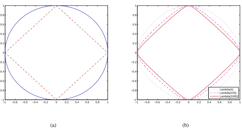
A more explicit illustration of the entropic regularization under a Laplace MaxEnDNet, compar-ing to the conventional L1and L2regularization over an M3N, can be seen in Figure 2, where the
fea-sible regions due to the three different norms used in the regularizer are plotted in a two dimensional space. Specifically, it shows (1) L2-norm: w21+w22≤1; (2) L1-norm:|w1|+|w2| ≤1; and (3)
KL-norm:5
q
w2
1+1/λ+ q
w2
2+1/λ−(1/ √
λ)log(qλw2
1+1/2+1/2)−(1/ √
λ)log(qλw2
1+1/2+
1/2)≤b, where b is a parameter to make the boundary pass the(0,1)point for easy comparison with the L2and L1curves. It is easy to show that b equals to
p
1/λ+p
1+1/λ−(1/√λ)log(√λ+1/2+ 1/2). It can be seen that the L1-norm boundary has sharp turning points when it passes the axises,
whereas the L2 and KL-norm boundaries turn smoothly at those points. This is the intuitive
ex-planation of why the L1-norm directly gives sparse estimators, whereas the L2-norm and
KL-norm due to a Laplace prior do not. But as shown in Figure 2(b), when the λ gets larger and larger, the KL-norm boundary moves closer and closer to the L1-norm boundary. When λ→∞, q
w2
1+1/λ+ q
w2
2+1/λ−(1/ √
λ)log(qλw2
1+1/2+1/2)−(1/ √
λ)log(qλw2
1+1/2+1/2)→ |w1|+|w2|and b→1, which yields exactly the L1-norm in the two dimensional space. Thus, under
the linear model assumption of the discriminant functions F(·; w), our framework can be seen as a smooth relaxation of the L1-M3N.
5. Variational Learning of Laplace MaxEnDNet
Although Theorem 2 seems to offer a general closed-form solution to p(w)under an arbitrary prior p0(w), in practice the Lagrange multipliersαi(y)in p(w)can be very hard to estimate from the dual
problem D1 except for a few special choices of p0(w), such as a normal as shown in Theorem 3,
which can be easily generalized to any normal prior. When p0(w) is a Laplace prior, as we have
shown in Theorem 5 and Corollary 6, the corresponding dual problem or primal problem involves a complex objective function that is difficult to optimize. Here, we present a variational method for an approximate learning of the Laplace MaxEnDNet.
Our approach is built on the hierarchical interpretation of the Laplace prior as shown in Equation (4). Replacing the p0(w)in Problem P1 with Equation (4), and applying the Jensen’s inequality, we
get an upper bound of the KL-divergence:
KL(p||p0) =−H(p)− hlog
Z
p(w|τ)p(τ|λ)dτip
4. Asλ→∞, the logarithm terms inkµkKLdisappear because of the fact thatlog xx →0 when x→∞.
−1 −0.8 −0.6 −0.4 −0.2 0 0.2 0.4 0.6 0.8 1 −1
−0.8 −0.6 −0.4 −0.2 0 0.2 0.4 0.6 0.8 1
(a)
−1 −0.8 −0.6 −0.4 −0.2 0 0.2 0.4 0.6 0.8 1 −1
−0.8 −0.6 −0.4 −0.2 0 0.2 0.4 0.6 0.8 1
Lambda(4) Lambda(100) Lambda(1000)
(b)
Figure 2: (a) L2-norm (solid line) and L1-norm (dashed line); (b) KL-norm with different Laplace
priors.
≤ −H(p)− h Z
q(τ)logp(w|τ)p(τ|λ) q(τ) dτip
,
L
(p(w),q(τ)),where q(τ)is a variational distribution used to approximate p(τ|λ). The upper bound is in fact a KL-divergence:
L
(p(w),q(τ)) =KL(p(w)q(τ)||p(w|τ)p(τ|λ)). Thus,L
is convex over p(w), and q(τ), respectively, but not necessarily joint convex over(p(w),q(τ)).Substituting this upper bound for the KL-divergence in P1, we now solve the following Varia-tional MaxEnDNet problem,
P1′(vMEDN): min
p(w)∈F1;q(τ);ξ
L
(p(w),q(τ)) +U(ξ).P1′can be solved with an iterative minimization algorithm alternating between optimizing over (p(w),ξ)and q(τ), as outlined in Algorithm 1, and detailed below.
Step 1: Keep q(τ)fixed, optimize P1′with respect to(p(w),ξ). Using the same procedure as in solving P1, we get the posterior distribution p(w)as follows,
p(w) ∝exp{
Z
q(τ)log p(w|τ)dτ−b} ·exp{w⊤η−
∑
i,y6=yi
αi(y)∆ℓi(y)}
∝exp{−1
2w
⊤hA−1
iqw−b+w⊤η−
∑
i,y6=yiαi(y)∆ℓi(y)}
Algorithm 1 Variational MaxEnDNet
Input: data
D
={hxi,yii}Ni=1, constants C andλ, iteration number TOutput: posterior meanhwiT p
Initializehwi1p←0,Σ1←I
for t=1 to T−1 do
Step 1: solve (9) or (10) forhwitp+1=Σtη; updatehww⊤it+1
p ←Σt+hwitp+1(hwitp+1)⊤.
Step 2: use (11) to updateΣt+1←diag(
q hw2
ki t+1 p
λ ).
end for
whereη=∑i,y6=yiαi(y)∆fi(y), A=diag(τk), and b=KL(q(τ)||p(τ|λ))is a constant. The posterior mean and variance arehwip=µ=ΣηandΣ= (hA−1iq)−1=hww⊤ip− hwiphwi⊤p, respectively.
Note that this posterior distribution is also a normal distribution. Analogous to the proof of Theorem 3, we can derive that the dual parametersαare estimated by solving the following dual problem:
max
α
∑
i,y6=yi
αi(y)∆ℓi(y)−
1 2η
⊤Ση (9)
s.t.
∑
y6=yiαi(y) =C; αi(y)≥0,∀i,∀y6=yi.
This dual problem is now a standard quadratic program symbolically identical to the dual of an M3N, and can be directly solved using existing algorithms developed for M3N, such as the SMO (Taskar et al., 2003) and the exponentiated gradient (Bartlett et al., 2004) methods. Alternatively, we can solve the following primal problem:
min w,ξ
1 2w
⊤Σ−1w+C
∑
N i=1ξi (10)
s.t. w⊤∆fi(y)≥∆ℓi(y)−ξi;ξi≥0, ∀i,∀y6=yi.
Based on the proof of Corollary 4, it is easy to show that the solution of the problem (10) leads to the posterior mean of w under p(w), which will be used to do prediction by h1. The primal problem
can be solved with the subgradient (Ratliff et al., 2007), cutting-plane (Tsochantaridis et al., 2004), or extragradient (Taskar et al., 2006) method.
Step 2: Keep p(w) fixed, optimize P1′ with respect to q(τ). Taking the derivative of
L
with respect to q(τ)and set it to zero, we get:q(τ) ∝p(τ|λ)exp{hlog p(w|τ)ip}.
Since both p(w|τ)and p(τ|λ)can be written as a product of univariate Gaussian and univariate ex-ponential distributions, respectively, over each dimension, q(τ)also factorizes over each dimension: q(τ) =∏Kk=1q(τk), where each q(τk)can be expressed as:
∀k : q(τk) ∝p(τk|λ)exp{hlog p(wk|τk)ip}
∝
N
(q
hw2kip|0,τk)exp(−
The same distribution has been derived by Kaban (2007), and similar to the hierarchical
rep-resentation of a Laplace distribution we can get the normalization factor: R
N
(q
hw2kip|0,τk)·
λ
2exp(− 1
2λτk)dτk = √
λ
2 exp(− q
λhw2
kip). Also, we can calculate the expectations hτ− 1
k iq which
are required in calculatinghA−1iqas follows,
hτ1 kiq
=
Z 1
τk
q(τk)dτk = s
λ
hw2kip
. (11)
We iterate between the above two steps until convergence. Due to the convexity (not joint convexity) of the upper bound, the algorithm is guaranteed to converge to a local optimum. Then, we apply the posterior distribution p(w), which is in the form of a normal distribution, to make prediction using the averaging prediction law in Equation (2). Due to the shrinkage effect of the Laplacian entropic regularization discussed in Section 4, for irrelevant features, the variances should converge to zeros and thus lead to a sparse estimation of w. To summarize, the intuition behind this iterative minimization algorithm is as follows. First, we use a Gaussian distribution to approximate the Laplace distribution and thus get a QP problem that is analogous to that of the standard M3N; then, in the second step we update the covariance matrix in the QP problem with an exponential hyper-prior on the variance.
6. Generalization Bound
The PAC-Bayes theory for averaging classifiers (McAllester, 1999; Langford et al., 2001) provides a theoretical motivation to learn an averaging model for classification. In this section, we extend the classic PAC-Bayes theory on binary classifiers to MaxEnDNet, and analyze the generalization performance of the structured prediction rule h1 in Equation (2). In order to prove an error bound
for h1, the following mild assumption on the boundedness of discriminant function F( ·; w) is
necessary, that is, there exists a positive constant c, such that,
∀w, F(·; w)∈
H
:X
×Y
→[−c,c].Recall that the averaging structured prediction function under the MaxEnDNet is defined as h(x,y) =
hF(x,y; w)ip(w). Let’s define the predictive margin of an instance (x,y) under a function h as M(h,x,y) =h(x,y)−maxy′6=yh(x,y′). Clearly, h makes a wrong prediction on (x,y) only if
M(h,x,y)≤0. Let Q denote a distribution over
X
×Y
, and letD
represent a sample of N in-stances randomly drawn from Q. With these definitions, we have the following structured version of PAC-Bayes theorem.Theorem 8 (PAC-Bayes Bound of MaxEnDNet) Let p0 be any continuous probability
distribu-tion over
H
and letδ∈(0,1). If F(·; w)∈H
is bounded by±c as above, then with probability at least 1−δ, for a random sampleD
of N instances from Q, for every distribution p overH
, and for all margin thresholdsγ>0:PrQ(M(h,x,y)≤0)≤PrD(M(h,x,y)≤γ) +O
r
γ−2KL(p||p
0)ln(N|
Y
|) +ln N+lnδ−1N
where PrQ(.)and PrD(.)represent the probabilities of events over the true distribution Q, and over
the empirical distribution of
D
, respectively.The proof of Theorem 8 follows the same spirit of the proof of the original PAC-Bayes bound, but with a number of technical extensions dealing with structured outputs and margins. See ap-pendix B.5 for the details.
Recently, McAllester (2007) presents a stochastic max-margin structured prediction model, which is different from the averaging predictor under the MaxEnDNet model, by defining/designing a “posterior” distribution from which a model is sampled to make prediction, and achieves a PAC-Bayes bound which holds for arbitrary models sampled from the particular posterior distribution. Langford and Shawe-Taylor (2003) show an interesting connection between the PAC-Bayes bounds for averaging classifiers and stochastic classifiers, again by designing a posterior distribution. But our posterior distribution is solved with MaxEnDNet and is generally different from those designed by McAllester (2007) and Langford and Shawe-Taylor (2003).
7. Experiments
In this section, we present empirical evaluations of the proposed Laplace MaxEnDNet (LapMEDN) on both synthetic and real data sets. We compare LapMEDN with M3N (i.e., the Gaussian MaxEnD-Net), L1-regularized M3N (L1-M3N), CRFs, L1-regularized CRFs (L1-CRFs), and L2-regularized
CRFs (L2-CRFs). We use the quasi-Newton method (Liu and Nocedal, 1989) and its variant
(An-drew and Gao, 2007) to solve the optimization problem of CRFs, L1-CRFs, and L2-CRFs. For M3N
and LapMEDN, we use the exponentiated gradient method (Bartlett et al., 2004) to solve the dual QP problem; and we also use the sub-gradient method (Ratliff et al., 2007) to solve the correspond-ing primal problem. To the best of our knowledge, no formal description, implementation, and evaluation of the L1-M3N exist in the literature, therefore for comparison purpose we had to
de-velop this model and algorithm anew. Details of our work along this line was reported in Zhu et al. (2009b), which is beyond the scope of this paper. But briefly, for our experiments on synthetic data, we implemented the constraint generating method (Tsochantaridis et al., 2004) which uses MOSEK to solve an equivalent LP re-formulation of L1-M3N. However, this approach is extremely slow on
larger problems; therefore on real data we instead applied the sub-gradient method (Ratliff et al., 2007) with a projection to an L1-ball (Duchi et al., 2008) to solve the larger L1-M3N based on the
equivalent re-formulation with an L1-norm constraint (i.e., the second formulation in Appendix A). 7.1 Evaluation on Synthetic Data
We first evaluate all the competing models on synthetic data where the true structured predictions are known. Here, we consider sequence data, that is, each input x is a sequence(x1, . . . ,xL), and each
component xl is a d-dimensional vector of input features. The synthetic data are generated from
pre-specified conditional random field models with either i.i.d. instantiations of the input features (i.e., elements in the d-dimensional feature vectors) or correlated (i.e., structured) instantiations of the input features, from which samples of the structured output y, that is, a sequence(y1, . . . ,yL),
7.1.1 I.I.D. INPUTFEATURES
The first experiment is conducted on synthetic sequence data with 100 i.i.d. input features (i.e., d=100). We generate three types of data sets with 10, 30, and 50 relevant input features, respec-tively. For each type, we randomly generate 10 linear-chain CRFs with 8 binary labeling states (i.e., L=8 and
Y
l={0,1}). The feature functions include: a real valued state-feature function over a one dimensional input feature and a class label; and 4 (2×2) binary transition feature functions captur-ing pairwise label dependencies. For each model we generate a data set of 1000 samples. For each sample, we first independently draw the 100 input features from a standard normal distribution, and then apply a Gibbs sampler (based on the conditional distribution of the generated CRFs) to assign a labeling sequence with 5000 iterations.For each data set, we randomly draw a subset as training data and use the rest for testing. The sizes of training set are 30, 50, 80, 100, and 150. The QP problem in M3N and the first
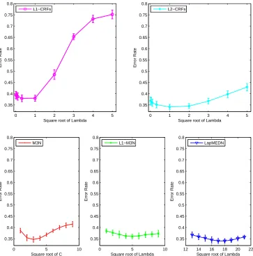
step of LapMEDN is solved with the exponentiated gradient method (Bartlett et al., 2004). In all the following experiments, the regularization constants of L1-CRFs and L2-CRFs are chosen from {0.01,0.1,1,4,9,16}by a 5-fold cross-validation during the training. For the LapMEDN, we use the same method to chooseλfrom 20 roughly evenly spaced values between 1 and 268. For each setting, a performance score is computed from the average over 10 random samples of data sets.
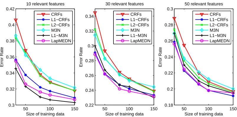
The results are shown in Figure 3. All the results of the LapMEDN are achieved with 3 itera-tions of the variational learning algorithm. From the results, we can see that under different settings LapMEDN consistently outperforms M3N and performs comparably with L1-CRFs and L1-M3N,
both of which encourage a sparse estimate; and both the L1-CRFs and L2-CRFs outperform the
un-regularized CRFs, especially in the cases where the number of training data is small. One in-teresting result is that the M3N and L2-CRFs perform comparably. This is reasonable because as
derived by Lebanon and Lafferty (2001) and noted by Globerson et al. (2007) that the L2-regularized
maximum likelihood estimation of CRFs has a similar convex dual as that of the M3N, and the only
difference is the loss they try to optimize, that is, CRFs optimize the log-loss while M3N optimizes the hinge-loss. Another interesting observation is that when there are very few relevant features, L1-M3N performs the best (slightly better than LapMEDN); but as the number of relevant features
increases LapMEDN performs slightly better than the L1-M3N. Finally, as the number of training
data increases, all the algorithms consistently achieve better performance.
7.1.2 CORRELATEDINPUTFEATURES
In reality, most data sets contain redundancies and the input features are usually correlated. So, we evaluate our models on synthetic data sets with correlated input features. We take the similar procedure as in generating the data sets with i.i.d. features to first generate 10 linear-chain CRF models. Then, each CRF is used to generate a data set that contain 1000 instances, each with 100 input features of which 30 are relevant to the output. The 30 relevant input features are partitioned into 10 groups. For the features in each group, we first draw a real-value from a standard normal distribution and then corrupt the feature with a random Gaussian noise to get 3 correlated features. The noise Gaussian has a zero mean and standard variance 0.05. Here and in all the remaining experiments, we use the sub-gradient method (Ratliff et al., 2007) to solve the QP problem in both M3N and the variational learning algorithm of LapMEDN. We use the learning rate and complexity constant that are suggested by the authors, that is,αt =2β1√t and C=200β, whereβis a parameter
50 100 150 0.3 0.32 0.34 0.36 0.38 0.4 0.42
Size of training data
Error Rate
10 relevant features
CRFs L1−CRFs L2−CRFs M3N L1−M3N LapMEDN
50 100 150 0.22 0.24 0.26 0.28 0.3 0.32 0.34
Size of training data
Error Rate
30 relevant features
CRFs L1−CRFs L2−CRFs M3N L1−M3N LapMEDN
50 100 150 0.18 0.2 0.22 0.24 0.26 0.28 0.3
Size of training data
Error Rate
50 relevant features
CRFs L1−CRFs L2−CRFs M3N L1−M3N LapMEDN
Figure 3: Evaluation results on data sets with i.i.d features.
50 100 150 200 250
0.2 0.21 0.22 0.23 0.24 0.25 0.26 0.27 0.28
Size of training data
Error Rate CRFs L1−CRFs L2−CRFs M3N L1−M3N LapMEDN
Figure 4: Results on data sets with 30 relevant features.
10 data sets as the final results. Like the method of Taskar et al. (2003), in each run we choose one part to do training and test on the rest K-1 parts. We vary K from 20, 10, 7, 5, to 4. In other words, we use 50, 100, about 150, 200, and 250 samples during the training. We use the same grid search to chooseλandβfrom{9,16,25,36,49,64}and{1,10,20,30,40,50,60}respectively. Results are shown in Figure 4. We can get the same conclusions as in the previous results.
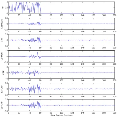
Figure 5 shows the true weights of the corresponding 200 state feature functions in the model that generates the first data set, and the average of estimated weights of these features under all competing models fitted from the first data set. All the averages are taken over 10 fold cross-validation. From the plots (2 to 7) of the average model weights, we can see that: for the last 140 state feature functions, which correspond to the last 70 irrelevant features, their average weights under LapMEDN (averaged posterior means w in this case), L1-M3N and L1-CRFs are extremely
small, while CRFs and L2-CRFs can have larger values; for the first 60 state feature functions, which
0 20 40 60 80 100 120 140 160 180 200 0
0.5 1
W
0 20 40 60 80 100 120 140 160 180 200
−0.5 0 0.5
LapMEDN
0 20 40 60 80 100 120 140 160 180 200
−0.5 0 0.5
M3N
0 20 40 60 80 100 120 140 160 180 200
−0.5 0 0.5
L1−M3N
0 20 40 60 80 100 120 140 160 180 200
−2 0 2
CRF
0 20 40 60 80 100 120 140 160 180 200
−0.5 0 0.5
L2−CRF
0 20 40 60 80 100 120 140 160 180 200
−0.5 0 0.5
State Feature Functions
L1−CRF
Figure 5: From top to bottom, plot 1 shows the weights of the state feature functions in the linear-chain CRF model from which the data are generated; plot 2 to plot 7 show the average weights of the learned LapMEDN, M3N, L1-M3N, CRFs, L2-CRFs, and L1-CRFs over
10 fold CV, respectively.
0 10 20 30 40 50 60 70 80 90 100
2 3 4x 10
−3
Features
Var of LapMEDN