Network Granger Causality with Inherent Grouping
Structure
Sumanta Basu [email protected]
Department of Statistics University of Michigan
Ann Arbor, MI 48109-1092, USA
Ali Shojaie [email protected]
Department of Biostatistics University of Washington Seattle, WA, USA
George Michailidis [email protected]
Department of Statistics University of Michigan
Ann Arbor, MI 48109-1092, USA
Editor:Bin Yu
Abstract
The problem of estimating high-dimensional network models arises naturally in the analysis of many biological and socio-economic systems. In this work, we aim to learn a network structure from temporal panel data, employing the framework of Granger causal models under the assumptions of sparsity of its edges and inherent grouping structure among its nodes. To that end, we introduce a group lasso regression regularization framework, and also examine a thresholded variant to address the issue of group misspecification. Further, the norm consistency and variable selection consistency of the estimates are established, the latter under the novel concept of direction consistency. The performance of the proposed methodology is assessed through an extensive set of simulation studies and comparisons with existing techniques. The study is illustrated on two motivating examples coming from functional genomics and financial econometrics.
Keywords: Granger causality, high dimensional networks, panel vector autoregression model, group lasso, thresholding
1. Introduction
and volume (Hiemstra and Jones, 1994), etc. More recently the Granger causal framework has found diverse applications in biological sciences including functional genomics, systems biology and neurosciences to understand the structure of gene regulation, protein-protein interactions and brain circuitry, respectively.
It should be noted that the concept of Granger causality is based on associations be-tween time series, and only under very stringent conditions, true causal relationships can be inferred (Pearl, 2000). Nonetheless, this framework provides a powerful tool for under-standing the interactions among random variables based on time course data.
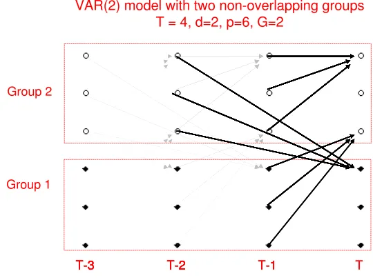
Network Granger causality (NGC) extends the notion of Granger causality among two variables to a wider class of pvariables. Such extensions involving multiple time series are handled through the analysis of vector autoregressive processes (VAR) (L¨utkepohl, 2005). Specifically, forpstationary time seriesX1t, . . . , Xpt, with Xt= (X1t, . . . , Xpt)0, one considers the class of models
Xt=A1Xt−1+. . .+AdXt−d+t, (1)
where A1, A2, . . . , Ad are p×p real-valued matrices, dis the unknown order of the VAR model and the innovation process satisfies t ∼ N(0, σ2I). In this model, the time series
{Xjt} is said to be Granger causal for the time series{Xit}ifAhi,j 6= 0 for someh= 1, . . . , d.
Equivalently we can say that there exists an edge Xjt−h → Xit in the underlying network model comprising of (d+ 1)×p nodes (see Figure 1). We call A1, . . . , Ad the adjacency matrices from lags 1, . . . , d. Note that the entries Ahij of the adjacency matrices are not binary indicators of presence/absence of edges between two nodes Xt
i and X
t−h
j . Rather,
they represent the direction and strength of influence from one node to the other.
T T-1
T-2 T-3
Group 1 Group 2
VAR(2) model with two non-overlapping groups T = 4, d=2, p=6, G=2
T-2
T-3 T-2 T-1
T-3 T-2 T-1 T
T-3
The temporal structure induces a natural partial order among the nodes of this network, which in turn simplifies significantly the corresponding estimation problem (Shojaie and Michailidis, 2010a) of a directed acyclic graph. Nevertheless, one still has to deal with estimating a high-dimensional network (e.g., hundreds of genes) from a limited number of samples.
The traditional asymptotic framework of estimating VAR models requires observing a long, stationary realization {X1, . . . , XT, T → ∞, p, dfixed} of the p-dimensional time series. This is not appropriate in many biological applications for the following reasons. First, long stationary time series are rarely observed in these contexts. Second, the number of time series (p) being large compared toT, the task of consistent order (d) selection using standard criteria (e.g., AIC or BIC) becomes challenging. Similar issues arise in many econometric applications where empirical evidence suggests lack of stationarity over a long time horizon, although the multivariate time series exhibits locally stable distributional properties.
A more suitable framework comes from the study of panel data, where one observes several replicates of the time series, with possibly short T, across a panel of nsubjects. In biological applications replicates are obtained from test subjects. In the analysis of macroe-conomic variables, households or firms typically serve as replicates. After removing panel specific fixed effects one treats the replicates as independent samples, performs regression analysis under the assumption of common slope structure and studies the asymptotic prop-erties under the regime n → ∞. Recent works of Cao and Sun (2011) and Binder et al. (2005) analyze theoretical properties of short panel VARs in the low-dimensional setting
(n→ ∞, T, p fixed).
The focus of this work is on estimating a high-dimensional NGC model in the panel data context (p, nlarge, T small to moderate). This work is motivated by two application domains, functional genomics and financial econometrics. In the first application (presented in Section 6) one is interested in reconstructing a gene regulatory network structure from time course data, a canonical problem in functional genomics (Michailidis, 2012). The second motivating example examines the composition of balance sheets of the n = 50 largest US banks by size, over T = 9 quarterly periods, which provides insight into their risk profile.
The nature of high-dimensionality in these two examples comes from both estimation of
p2 coefficients for each of the adjacency matricesA1, . . . , Ad, but also from the fact that the order of the time seriesdis often unknown. Thus, in practice, one must either “guess” the order of the time series (often times, it is assumed that the data is generated from a VAR(1) model, which can result in significant loss of information), or include all of the past time points, resulting in significant increase in the number of variables in cases where d T. Thus, efficient estimation of the order of the time series becomes crucial.
Latent variable based dimension reduction techniques like principal component analysis or factor models are not very useful in this context since our goal is to reconstruct a network among the observed variables. To achieve dimension reduction we impose a group sparsity assumption on the structure of the adjacency matrices A1, . . . , Ad. In many applications,
be incorporated to the Granger causality framework through a group lasso penalty. If the group specification is correct it enables estimation of denser networks with limited sample sizes (Bach, 2008; Huang and Zhang, 2010; Lounici et al., 2011). However, the group lasso penalty can achieve model selection consistency only at a group level. In other words, if the groups are misspecified, this procedure can not perform within group variable selection (Huang et al., 2009), an important feature in many applications.
Over the past few years, several authors have adopted the framework of network Granger causality to analyze multivariate temporal data. For example, Fujita et al. (2007) and Lozano et al. (2009) employed NGC models coupled with penalized `1 regression methods to learn gene regulatory mechanisms from time course microarray data. Specifically, Lozano et al. (2009) proposed to group all the past observations, using a variant of group lasso penalty, in order to construct a relatively simple Granger network model. This penalty takes into account the average effect of the covariates over different time lags and connects Granger causality to this average effect being significant. However, it suffers from significant loss of information and makes the consistent estimation of the signs of the edges difficult (due to averaging). Shojaie and Michailidis (2010b) proposed a truncating lasso approach by introducing a truncation factor in the penalty term, which strongly penalizes the edges from a particular time lag, if it corresponds to a highly sparse adjacency matrix.
Despite recent use of NGC in applications involving high dimensional data, theoretical properties of the resulting estimators have not been fully investigated. For example, Lozano et al. (2009) and Shojaie and Michailidis (2010b) discuss asymptotic properties of the re-sulting estimators, but neither addresses in depth norm consistency properties, nor do they examine under what vector autoregressive structures the obtained results hold.
In this paper, we develop a general framework that accommodates different variants of group lasso penalties for NGC models. It allows for the simultaneous estimation of the order of the times series and the Granger causal effects; further, it allows for variable selection even when the groups are misspecified. In summary, the key contributions of this work are: (i) investigate in depthsufficient conditions that explicitly take into consideration the structure of the VAR(d) model to establish norm consistency, (ii) introduce the novel notion
of direction consistency, which generalizes the concept of sign consistency and provides
insight into the properties of group lasso estimates within a group, and (iii) use the latter notion to introduce an easy to compute thresholded variant of group lasso, that performs within group variable selection in addition to group sparsity pattern selection even when the group structure is misspecified.
All the obtained results are non-asymptotic in nature, and hence help provide insight into the properties of the estimates under different asymptotic regimes arising from varying growth rates of T, p, n, group sizes and the number of groups.
2. Model and Framework
Notation. Consider a VAR model
Xt
|{z}
p×1 = A1
|{z}
p×p
observed over T time points t = 1, . . . , T, across n panels. The index set of the variables
Np ={1,2, . . . , p} can be partitioned into G non-overlapping groups Gg, i.e., Np =∪Gg=1Gg
and Gg ∩ Gg0 = φ ifg 6= g0. Also kg =|Gg| denotes the size of the gth group with kmax =
max
1≤g≤Gkg. In general, we use λmin and λmax to denote the minimum and maximum of a
finite collection of numbersλ1, . . . , λm.
For any matrix A, we denote theith row byAi:,jthcolumn by A:j and the collection of
rows (columns) corresponding to thegth group byA[g]:(A:[g]). The transpose of a matrixA
is denoted by A0 and its Frobenius norm by ||A||F. For a symmetric/Hermitian matrix Σ,
its maximum and minimum eigenvalues are denoted by Λmin(Σ) and Λmax(Σ), respectively. The symbolA1:h is used to denote the concatenated matrix
A1 :· · ·:Ah
, for any h >0. For any matrix or vector D, kDk0 denotes the number of non-zero coordinates in D. For notational convenience, we reserve the symbolk.kto denote the `2 norm of a vector and/or the spectral norm of a matrix. For a pre-defined set of non-overlapping groupsG1, . . . ,GG
on {1, . . . , p}, the mixed norms of vectors v ∈Rp are defined as kvk2,1 = PGg=1kv[g]k and
kvk2,∞ = max1≤g≤Gkv[g]k. Also for any vector β, we use βj to denote its jth coordinate
and β[g] to denote the coordinates corresponding to thegth group. We also use supp(v) to
denote the support ofv, i.e., supp(v) ={j ∈ {1, . . . , p}|vj 6= 0}.
Network Granger causal (NGC) estimates with group sparsity. Consider n
replicates from the NGC model (2), and denote the n×p observation matrix at timet by
Xt. In econometric applications the data on p economic variables across n panels (firms,
households etc.) can be observed over T time points. For time course microarray data one typically observes the expression levels of pgenes acrossnsubjects overT time points. After removing the panel specific fixed effects one assumes the common slope structure and independence across the panels. The data are high-dimensional if either T or p is large compared to n. In such a scenario, we assume the existence of an underlying group sparse structure, i.e., for everyi= 1, . . . , p, the support of theithrow ofA1:T−1 =
A1 :· · ·:AT−1 in the model (2) can be covered by a small number of groupssi, wheresi (T−1)G. Note that the groups can be misspecified in the sense that the coordinates of a group covering the support need not be all non-zero. Hence, for a properly specified group structure we shall expect si kA1:i:Tk0. On the contrary, with many misspecified groups, si can be of the same order, or even larger than kA1:i:Tk0.
Learning the network of Granger causal effects {(i, j)∈ {1, . . . , p}:Atij 6= 0 for some t}
is equivalent to recovering the correct sparsity pattern inA1:(T−1) and consistently estimat-ing the non-zero effectsAtij. In the high-dimensional regression problems this is achieved by simultaneous regularization and selection operators like lasso and group lasso. The group Granger causal estimates of the adjacency matrices A1, . . . , AT−1 are obtained by solving the following optimization problem
ˆ
A1:T−1= argmin
A1,···,AT−1
1 2n
XT −
T−1 X
t=1
XT−t At0
2
F
+λ T−1 X
t=1
p
X
i=1
G
X
g=1
wi,gt kAti:[g]k, (3)
where Xt is the n×p observation matrix at time t, constructed by stacking n replicates
regularization parameter. The optimization problem can be separated into the following p
penalized regression problems:
ˆ
A1:i:T−1= argmin
θ1,···,θT−1∈
Rp
1 2nkX
T
:i − T−1 X
t=1
XT−tθtk2+λ T−1 X
t=1
G
X
g=1
wti,gkθt[g]k, i= 1,· · · , p. (4)
The orderdof the VAR model is estimated as ˆd= max
1≤t≤T−1{t: ˆA
t6=0}.
Different choices of weightswti:g lead to different variants of NGC estimates. The regular NGC estimates correspond to the choices wti,g = 1 or pkg, while for adaptive group NGC
estimates the weights are chosen aswi,gt = Aˆ
t i:[g]
−1
, where ˆAt are obtained from a regular
NGC estimation. For ˆAti:[g] = 0, the weight wi,gt is infinite, which is interpreted as discarding the variables in group g from the optimization problem.
Thresholded NGC estimates are calculated by a two-stage procedure. The first stage involves a regular NGC estimation procedure. The second stage uses a bi-level thresholding strategy on the estimates ˆAt. First, the estimated groups with`2norm less than a threshold
(δgrp=cλ, c >0) are set to zero. The second level of thresholding (within group) is applied
if thea prioriavailable grouping information is not entirely reliable. ˆAtijwithin an estimated
group ˆAt
i:[g] is thresholded to zero if
ˆ
At
ij
/
ˆ
At
i:[g]
is less than a thresholdδmisspec ∈(0,1). So, for every t= 1, . . . , T −1, ifj∈ Gg, the thresholded NGC estimates are
˜
Atij = ˆAtijIn
ˆ
Atij
≥δmisspec
ˆ
Ati:[g]
o
In
ˆ
Ati:[g]
≥δgrp
o
.
The tuning parameters λgrp and δmisspec are chosen via cross-validation. The rationale behind this thresholding strategy is discussed in Section 4.
3. Estimation Consistency of NGC estimates
In this section we establish the norm consistency of regular group NGC estimates. The regular NGC estimates in (3) are obtained by solving p separate group lasso programs with a common design matrix Xn×p(T−1) = [X1 : · · · : XT−1]. This design matrix has ¯
p= (T−1)pcolumns which can be partitioned into ¯G= (T−1)Ggroups{G1, . . . ,GG¯}. We denote the sample Gram matrix by C =X0X/n. For the ith optimization problem, these
¯
G= (T −1)Ggroups are penalized byλ(t−1)G+g :=λ wi,gt , 1≤t≤T −1, 1≤g≤G, with
the choice of weights wti,g described in Section 2. Following Lounici et al. (2011) one can establish a non-asymptotic upper bound on the `2 estimation error of the NGC estimates
ˆ
ForL >0, we say that aRestricted Eigenvalue(RE) assumption RE(s, L) is satisfied if there exists a positive number φRE=φRE(s)>0 such that
min
J⊂NG¯,|J|≤s
∆∈Rp¯\{0}
kX∆k √
nk∆[J]k : X
g∈Jc
λgk∆[g]k ≤L X
g∈J
λgk∆[g]k
≥φRE. (5)
The following proposition provides a non-asymptotic upper bound on the `2-estimation error of the group NGC estimates under RE assumptions. The proof follows along the lines of Lounici et al. (2011) and is delegated to Appendix C.
Proposition 3.1 Consider a regular NGC estimation problem (4)withsmax= max1≤i≤psi
and s=Pp
i=1si. Suppose λ in (3) is chosen large enough so that for someα >0,
λg ≥
2σ
√
n
q C[g][g]
p
kg+
π
√
2 q
α log ¯G
for everyg∈NG¯, (6)
Also assume that the common design matrix X = [X1 : · · · : XT−1] in the p regression
problems (4) satisfy RE(2smax,3). Then, with probability at least 1−2pG¯1−α,
ˆ
A1:T−1−A1:T−1
F
≤ 4
√
10
φ2RE(2smax)
λ2max
λmin
√
s. (7)
Remark. Consider a high-dimensional asymptotic regime where ¯G nB for some
B >0,kmax/kmin=O(1), s=O(na1) and kmax=O(na2) with 0< a1, a2< a1+a2 <1 so
that the total number of non-zero effects iso(n). If {kC[g][g]k, g∈NG¯} are bounded above (often accomplished by standardizing the data) andφ2RE(2smax) is bounded away from zero (see Proposition 3.2 for more details), then the NGC estimates are norm consistent for any choice ofα >2 +a2/B.
Note that group lasso achieves faster convergence rate (in terms of estimation and pre-diction error) than lasso if the groups are appropriately specified. For example, if all the groups are of equal sizekandλg =λfor allg, then group lasso can achieve an`2estimation error of orderO
√
s(√k+plog ¯G)/√n
. In contrast, lasso’s error is known to be of the
order O
p
kA1:dk
0 log ¯p/n
, which establishes that group lasso has a lower error bound if
s kA1:dk0. On the other hand, lasso will have a lower error bound ifs kA1:dk0, i.e., if the groups are highly misspecified.
Validity of RE assumption in Group NGC problems. In view of Theorem 3.1, it is important to understand how stringent the RE condition is in the context of NGC problems. It is also important to find a lower bound on the RE coefficientφRE, as it affects
the convergence rate of the NGC estimates. For the panel-VAR setting, we can rigorously establish that the RE condition holds with overwhelming probability, as long as n, pgrow at the same rate required for`2-consistency.
(X1)0, . . . ,(XT−1)00
. First, we exploit the spectral representation of the stationary VAR process to provide a lower bound on the minimum eigenvalue of Σ. In the next step, we establish a suitable deviation bound onX−Σ to prove thatX satisfies RE condition with high probability for sufficiently largen.
Proposition 3.2 (a) Suppose the VAR(d) model of (2) is stable, stationary. LetΣ be the
variance-covariance matrix of the(T−1)p-dimensional random variable (X1)0, . . . ,(XT−1)00.
Then the minimum eigenvalue of Σ satisfies
Λmin(Σ)≥σ2
max
θ∈[−π,π]
kA(e−iθ)k
−2
≥σ2
" 1 +
d
X
t=1
kAtk
#−2
≥σ2
1 +1
2(vin+vout) −2
,
where A(z) :=I−A1z−A2z2−. . .−Adzd is the reverse characteristic polynomial of the
VAR(d) process, and vin, vout are the maximum incoming and outgoing effects at a node,
cumulated across different lags
vin= d
X
t=1 max 1≤i≤p
p
X
j=1
|Atij|, vout= d
X
t=1 max 1≤j≤p
p
X
i=1
|Atij|.
(b) In addition, suppose the replicates from different panels are i.i.d. Then, for anys >0,
there exist universal positive constants ci such that if the sample size nsatisfies
n > Λ
2 max(Σ) Λ2
min(Σ)
(2 +Lλmax/λmin)4c0s(kmax+c1log(eG/¯ 2s)),
thenX satisfiesRE(s, L)with φ2RE ≥Λmin(Σ)/2 with probability at least 1−c2exp(−c3n).
Remark. Proposition 3.2 has two interesting consequences. First, it provides a lower bound on the RE constant φRE which is independent of T. So if the high dimensionality in the Granger causal network arises only from the time domain and not the cross-section
(T → ∞, p, Gfixed), the stationarity of the VAR process guarantees that the rate of
convergence depends only on the true order (d), and notT. Second, this result shows that the NGC estimates are consistent even if the node capacities vin and vout grow with n, p
at an appropriate rate.
4. Variable Selection Consistency of NGC estimates
In view of (4), to study the variable selection properties of NGC estimates it suffices to analyze the variable selection properties ofp generic group lasso estimates with a common design matrix.
effect. Several alternate penalized regression procedures have been proposed to overcome this shortcoming (Breheny and Huang, 2009; Huang et al., 2009). The main idea behind these procedures is to combine `2 and `1 norms in the penalty to encourage sparsity at both group and variable level. These estimators involve nonconvex optimization problems and are computationally expensive. Also their theoretical properties in a high dimensional regime are not well studied.
We take a different approach to deal with the issue of group misspecification. Although the group lasso penalty does not perform exact variable selection within groups, it performs regularization and shrinks the individual coefficients. We utilize this regularization to detect misspecification within a group. To this end, we formulate a generalized notion of sign consistency, henceforth referred as “direction consistency”, that provides insight into the properties of group lasso estimates within a single group. Subsequently, these properties are used to develop a simple, easy to compute, thresholded variant of group lasso which, in addition to group selection, achieves variable selection and sign consistency within groups. We consider a generic group lasso regression problem of the linear model y =Xβ0+
with p variables partitioned into G non-overlapping groups {G1, . . . ,GG} of size kg, g =
1, . . . , G. Without loss of generality, we assume β[0g] 6= 0 for g ∈ S = {1,2, . . . , s} and
β[0g]=0 for all g /∈S and consider the following group lasso estimate of β0:
ˆ
β= argmin
β∈Rp
1
2nkY−Xβk
2+
G
X
g=1
λgkβ[g]k, (8)
β0
|{z}
p×1
= [β[1]0 , . . . , β[0s]
| {z }
k1+...+ks=q
,0, . . . ,0 | {z }
p−q
] = [β(1)0 :β(2)0 ], (9)
X |{z}
n×p
= [X(1) | {z }
n×q
: X(2) | {z }
n×(p−q)
], C = 1
nX
0
X=
C11 C12
C21 C22
. (10)
Direction Consistency. For an m-dimensional vector τ ∈Rm\{0} define its
direc-tion vector D(τ) = τ /kτk , D(0) = 0. In the context of a generic group lasso regression (10), for a group g ∈ S of size kg, D(β[0g]) indicates the direction of influence of β[0g] at a
group level in the sense that it reflects the relative importance of the influential members within the group. Note that for kg = 1 the function D(·) simplifies to the usual sgn(·)
function.
Definition. An estimateβˆof a generic group lasso problem (8) isdirection consis-tent at a rateδn, if there exists a sequence of positive real numbers δn→0 such that
P
kD(βˆ[g])−D(β[0g])k< δn, ∀g∈S, βˆ[g]=0, ∀g /∈S
→1 as n, p→ ∞. (11)
Now suppose βˆ is a direction consistent estimator. Consider the set ˜Sgn := {j ∈ Gg :
|β0j|/kβ0[g]k> δn}. ˜Sgn can be viewed as a collection of influential group members within
a group Gg, which are “detectable” with a sample of size n. Then, it readily follows from
the definition that
The latter observation connects the precision of group lasso estimates to the accuracy of
a priori available grouping information. In particular, if the pre-specified grouping structure
is correct, i.e., all the members within a group have non-zero effects, then for a sufficiently large sample size we have ˜Sgn = Gg for all g ∈ S. Hence, if the group lasso estimate is direction consistent, it will correctly estimate the sign of all the variables in the support. On the other hand, in case of a misspecified a priori grouping structure (numerous zero coordinates in βg for g ∈ S), group lasso will correctly estimate only the signs of the
influential group members. This argument on zero vs. non-zero effects can be generalized to strong vs. weak effects, as well.
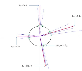
Example. We demonstrate the property of direction consistency using a small exam-ple. Consider a linear model with 8 predictors
y = 0.5x1−3x2+ 3x3+x4−2x5+ 3x8+e, e∼N(0,1).
The coefficient vectorβ0is partitioned into four groups of size 2, viz., (0.5,−3),(3,1),(−2,0) and (0,3). The last two groups are misspecified. We generated n = 25 samples from this model and ran group lasso regression with the above group structure. Figure 2 shows the true coefficient vectors (solid) and their estimates (dashed) from five iterations of the above exercise. Note that even though the`2 errors between β[0g] and ˆβ[g] vary largely across the four groups, the distance between their projections on the unit circle,
D(β
0
[g])−D( ˆβ[g]) , are comparatively stable across groups. In fact, Theorem 4.1 shows that under certain ir-representable conditions (IC) on the design matrix, it is possible to find a uniform (over all
g ∈S) upper boundδn on the `2 gap of these direction vectors. This motivates a natural thresholding strategy to correct for the misspecification in groups (cf. Proposition 4.2). Even though a group β[0g] is misspecified (i.e., lies on a coordinate axis), direction consis-tency ensures, with high probability, that the corresponding coordinate in D( ˆβ[g]) will be smaller than a thresholdδnwhich is common across all groups in the support.
Group Irrepresentable Conditions (IC). Next, we define the IC required for di-rection consistency of group lasso estimates. Irrepresentable conditions are common in the literature of high-dimensional regression problems (Zhao and Yu, 2006; van de Geer and B¨uhlmann, 2009) and are shown to be sufficient (and essentially necessary) for selection consistency of the lasso estimates. Further these conditions are known to be satisfied with high probability, if the population analogue of the Gram matrix belongs to the Toeplitz fam-ily (Zhao and Yu, 2006; Wainwright, 2009). In NGC estimation the population analogue of the Gram matrix Σ =V ar(X1:(T−1)) is block Toeplitz, so the irrepresentable assumptions are natural candidates for studying selection consistency of the estimates. Consider the notations of (8) and (10). Define K=diag(λ1Ik1, λ2Ik2, . . . , λsIks).
Uniform Irrepresentable Condition (IC) is satisfied if there exists 0< η <1 such that for allτ ∈Rq with kτk
2,∞= max
1≤g≤skτ[g]k2 ≤1,
1
λg
h
C21(C11)−1Kτ
i
[g]
<1−η, ∀g /∈S ={1, . . . , s}. (13)
β[4] = (0, 3)
β[1] = (0.5, -3)
β[2] = (3, 1)
β[3] = (-2, 0) D(β[1]) – D( β[1]
)
Figure 2: Example demonstrating direction consistency
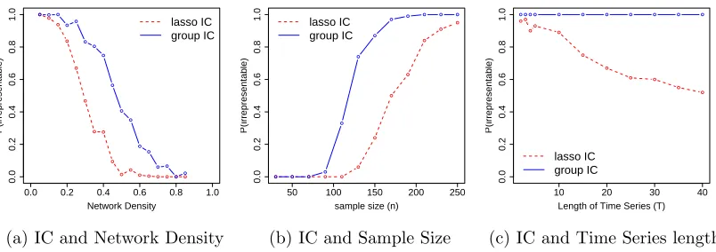
The IC is more stringent than the RE condition and is rarely met if the underlying model is not sparse. It can be shown that a slightly weaker version of this condition is necessary for direction consistency. We refer the readers to Appendix D for further discussion on the different irrepresentable assumptions and their properties. Numerical evidence suggests that the group IC tends to be less stringent than the IC required for the selection consistency of lasso. We illustrate this using three small simulated examples.
Simulation1. We constructed group sparse NGC models withT = 5, p= 21, G= 7, kg = 3
and different levels of network densities, where the network edges were selected at random and scaled so that kA1k= 0.1. For each of these models, we generated 100 samples of size
n= 150 and calculated the proportions of times the two types of irrepresentable conditions were met. The results are displayed in Figure 3a.
Simulation 2. We selected a VAR(1) model from the above class and generated samples
of size n = 20,50, . . . ,250. Figure 3b displays the proportions of times (based on 100 simulations) the two ICs were met.
Simulation 3. We generated n = 200 samples from the VAR(1) model of example 2
for T = 2,3,4,5,10, . . . ,40. Figure 3c displays the proportions of times (based on 100
0.0 0.2 0.4 0.6 0.8 1.0 0.0 0.2 0.4 0.6 0.8 1.0 Network Density P(irrepresentab le) ● ● ● ● ● ● ● ● ● ● ● ●● ●● ● ● ● ● ● ● ● ● ● ● ● ● ● ● ● ●● ● ● lasso IC group IC
(a) IC and Network Density
50 100 150 200 250
0.0 0.2 0.4 0.6 0.8 1.0
sample size (n)
P(irrepresentab le) ● ● ● ● ● ● ● ● ● ● ● ● ● ● ● ● ● ● ● ● ● ● ● ● lasso IC group IC
(b) IC and Sample Size
10 20 30 40
0.0 0.2 0.4 0.6 0.8 1.0
Length of Time Series (T)
P(irrepresentab le) ● ● ● ● ● ● ● ● ● ● ● ● ● ● ● ● ● ● ● ● ● ● lasso IC group IC
(c) IC and Time Series length
Figure 3: Comparison of lasso and group irrepresentable conditions in the context of group sparse NGC models. (a) group ICs tend to be met for dense networks where lasso IC fails to meet. (b) For the same network group IC is met with smaller sample size than required by lasso. (c) For longer time series group IC is satisfied more often than lasso IC.
Selection consistency for generic group lasso estimates. For simplicity, we dis-cuss the selection consistency properties of a generic group lasso regression problem with a common tuning parameter across groups, i.e.,λg =λfor everyg∈NG. Similar results can
be obtained for more general choices of the tuning parameters.
Theorem 4.1 Assume that the group uniform IC holds with 1−η for some η >0. Then,
for any choice of α >0,
λ ≥ max
g /∈S
1 η σ √ n r
(C22)[g][g]
p
kg+
π
√
2 p
α logG
and
δn ≥ max
g∈S 1 β 0 [g]
λ√s(C11)−1
+ σ √ n r (C11)
−1 [g][g]
p
kg+√π
2 p
αlog G
!
,
with probability greater than 1−4G1−α, there exists a solution βˆ satisfying
1. βˆ[g]= 0 for all g /∈S,
2.
ˆ
β[g]−β[0g]
< δn
β
0 [g]
, and hence
D( ˆβ[g])−D(β 0 [g])
< 2δn, for all g ∈ S. If
δn<1, then βˆ[g]6= 0 for all g∈S.
Thresholding in Group NGC estimators. As described in Section 2, regular group NGC estimates can be thresholded both at the group and coordinate levels. The first level of thresholding is motivated by the fact that lasso can select too many false positives [cf. van de Geer et al. (2011), Zhou (2010) and the references therein]. The second level of thresholding employs the direction consistency of regular group NGC estimates to perform within group variable selection with high probability. The following proposition demonstrates the benefit of these two types of thresholding. The second result is an immediate corollary of Theorem 4.1. Proof of the first result (thresholding at group level) requires some additional notations and is delegated to Appendix E.
Theorem 4.2 Consider a generic group lasso regression problem (8)with common tuning
parameter λg =λ.
(i) Assume the RE(s, 3) condition of (5) holds with a constant φRE and define βˆ[thgrpg] =
ˆ
β[g]1kβˆ[g]k>4λ. If
ˆ
S ={g ∈NG: ˆβ[thgrpg] 6=0}, then |Sˆ\S| ≤ φ2 s RE/12
, with probability at least
1−2G1−α.
(ii) Assume that uniform IC holds with 1−η for some η > 0. Choose λ and δn as in
Theorem 4.1 and define
ˆ
βjthgrp= ˆβj1{|βˆj|/kβˆ[g]k>2δn} for allj ∈ Gg.
Thensgn(βj0) =sgn( ˆβjthgrp) ∀j ∈Np with probability at least1−4G1−α, if min
j∈supp(β0)|β
0
j|>
2δnkβ[0g]k for allj ∈ Gg, i.e., if the effect of every non-zero member in a group is “visible”
relative to the total effect from the group.
5. Performance Evaluation
We evaluate the performances of regular, adaptive and thresholded variants of the group NGC estimators through an extensive simulation study, and compare the results to those obtained from lasso estimates. The R packagegrpreg(Breheny and Huang, 2009) was used to obtain the group lasso estimates. The settings considered are:
(a) Balanced groups of equal size: i.i.d samples of size n= 60,110,160 are generated from
lag-2 (d = 2) VAR models on T = 5 time points, comprising of p = 60,120,200 nodes partitioned into groups of equal size in the range 3-5.
(b) Unbalanced groups: We retain the same setting as before, however the corresponding
node set is partitioned into one larger group of size 10 and many groups of size 5.
(c)Misspecified balanced groups: i.i.d samples of sizen= 60,110,160 are generated from
lag-2 (d= 2) VAR models on T = 10 time points, comprising ofp= 60,120 nodes partitioned into groups of size 6. Further, for each group there is a 30% misspecification rate, namely that for every parent group of a downstream node, 30% of the group members do not exert any effect on it.
Using a 19 : 1 sample-splitting, the tuning parameter λ is chosen from an interval of the form [C1λe, C2λe], C1, C2 > 0, where λe =
p
2 log p/n for lasso and p2 logG/n for group lasso. The thresholding parameters are selected as δgrp = 0.7λσ at the group level
and δmisspec =n−0.2 within groups. These parameters are chosen by conducting a 20-fold
1
60
9 8 7 6 5 4 3 2 1
(a)
1
60
9 8 7 6 5 4 3 2 1
(b)
1
60
9 8 7 6 5 4 3 2 1
(c)
1
60
9 8 7 6 5 4 3 2 1
(d)
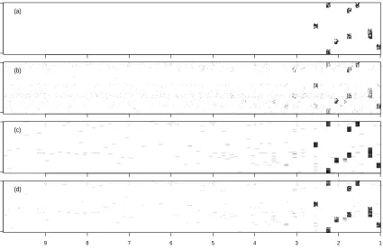
Figure 4: Estimated adjacency matrices of a misspecified NGC model with p = 60, T = 10, n = 60: (a) True, (b) Lasso, (c) Group Lasso, (d) Thresholded Group Lasso. The grayscale represents the proportion of times an edge was detected in 100 simulations.
[C3λ, C4λ] for δgrp and {n−δ, δ ∈[0,1]} forδmisspec. Finally, within group thresholding is applied only when the group structure is misspecified.
The following performance metrics were used for comparison purposes: (i) P recision=
T P/(T P +F P) , (ii) Recall=T P/(T P +F N) and (iii) Matthew’s Correlation coefficient (MCC) defined as
(T P ×T N)−(F P ×F N)
((T P +F P)×(T P +F N)×(T N+F P)×(T N +F N))1/2,
whereT P,T N,F P andF N correspond to true positives, true negatives, false positives and false negatives in the estimated network, respectively. The average and standard deviations (over 100 replicates) of the performance metrics are presented for each setup.
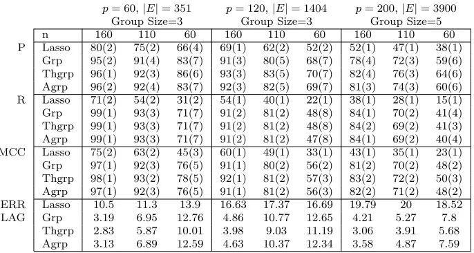
The results for the balanced settings are given in Table 1. The Recall for p= 60 shows that even for a network with 60×(5−1) = 240 nodes and |E|= 351 true edges, the group NGC estimators recover about 71% of the true edges with a sample size as low as n= 60, while lasso based NGC estimates recover only 31% of the true edges. The three group NGC estimates have comparable performances in all the cases. However thresholded lasso shows slightly higher precision than the other group NGC variants for smaller sample sizes (e.g.,
p= 60,|E|= 351 p= 120,|E|= 1404 p= 200,|E|= 3900 Group Size=3 Group Size=3 Group Size=5
n 160 110 60 160 110 60 160 110 60
P Lasso 80(2) 75(2) 66(4) 69(1) 62(2) 52(2) 52(1) 47(1) 38(1) Grp 95(2) 91(4) 83(7) 91(3) 80(5) 68(7) 78(4) 72(3) 59(6) Thgrp 96(1) 92(3) 86(6) 93(3) 83(5) 70(7) 82(4) 76(3) 64(6) Agrp 96(2) 92(4) 83(7) 92(3) 82(5) 69(7) 81(3) 74(3) 60(6) R Lasso 71(2) 54(2) 31(2) 54(1) 40(1) 22(1) 38(1) 28(1) 15(1) Grp 99(1) 93(3) 71(7) 91(2) 81(2) 48(8) 84(1) 70(2) 41(4) Thgrp 99(1) 93(3) 71(7) 91(2) 81(2) 48(8) 84(2) 69(2) 41(3) Agrp 99(1) 93(3) 71(7) 91(2) 81(2) 47(8) 84(1) 69(2) 40(4) MCC Lasso 75(2) 63(2) 45(3) 60(1) 49(1) 33(1) 43(1) 35(1) 23(1) Grp 97(1) 92(3) 76(5) 91(1) 80(2) 56(2) 81(2) 70(2) 48(2) Thgrp 98(1) 93(2) 78(5) 92(1) 81(2) 57(3) 83(2) 72(2) 50(3) Agrp 97(1) 92(3) 76(5) 91(1) 81(2) 56(3) 82(2) 71(2) 48(2) ERR Lasso 10.5 11.3 13.9 16.63 17.37 16.69 19.79 20 18.52 LAG Grp 3.19 6.95 12.76 4.86 10.77 12.65 4.21 5.27 7.8
Thgrp 2.83 5.87 10.01 3.98 9.03 11.19 3.06 3.91 5.68 Agrp 3.13 6.89 12.59 4.63 10.37 12.34 3.58 4.87 7.59
Table 1: Performance of different regularization methods in estimating graphical Granger causality with balanced group sizes and no misspecification; d = 2, T = 5,
SN R= 1.8. Precision (P), Recall (R), MCC are given in percentages (numbers in parentheses give standard deviations). ERR LAG gives the error associated with incorrect estimation of VAR order.
lasso is caused partially by its inability to estimate the order of the VAR model correctly, as measured by ERR LAG=Number of falsely connected edges from lags beyond the true order of the VAR model divided by the number of edges in the network (|E|). This finding is nicely illustrated in Figure 4 and Table 1. The group penalty encourages edges from the nodes of the same group to be picked up together. Since the nodes of the same group are also from the same time lag, the group variants have substantially lower ERR LAG. For example, average ERR LAG of lasso forp= 200, n= 160 is 19.79% while the average ERR LAGs for the group lasso variants are in the range 3.06%−4.21%.
The results for the unbalanced networks are given in Table 2. As in the balanced group setup, in almost all the simulation settings the group NGC variants outperform the lasso estimates with respect to all three performance metrics. However the performances of the different variants of group NGC are comparable and tend to have higher standard deviations than the lasso estimates. Also the average ERR LAGs for the group NGC variants are substantially lower than the average ERR LAG for lasso demonstrating the advantage of group penalty. Although the conclusions regarding the comparisons of lasso and group NGC estimates remain unchanged it is evident that the performances of all the estimators are affected by the presence of one large group, skewing the uniform nature of the network. For example the MCC measures of group NGC estimates in a balanced network with p = 60 and |E| = 351 vary around 97−98% which lowers to 89%−90% when the groups are unbalanced.
p= 60,|E|= 450 p= 120,|E|= 1575 p= 200,|E|= 4150 Groups=1×10,11×5 Groups=1×10,23×5 Groups=1×10,39×5
n 160 110 60 160 110 60 160 110 60
P Lasso 72(2) 69(3) 62(2) 51(1) 48(1) 41(1) 61(1) 53(1) 42(2) Grp 84(4) 79(6) 76(9) 55(5) 47(5) 40(6) 86(3) 77(5) 66(7) Thgrp 86(4) 82(7) 78(11) 60(6) 50(7) 40(5) 88(2) 79(6) 69(6) Agrp 85(3) 81(5) 77(9) 59(5) 51(5) 42(6) 88(2) 78(5) 67(6) R Lasso 45(2) 35(2) 22(2) 43(1) 34(1) 22(1) 23(1) 15(0) 7(0) Grp 94(3) 87(5) 61(8) 88(2) 75(5) 48(6) 73(3) 49(6) 22(5) Thgrp 95(2) 88(4) 62(8) 89(3) 77(4) 50(5) 73(3) 50(6) 21(5) Agrp 94(3) 87(5) 61(8) 88(2) 75(5) 48(6) 73(3) 49(6) 22(5) MCC Lasso 56(2) 48(2) 35(2) 46(1) 39(1) 29(1) 36(1) 28(1) 17(1) Grp 89(3) 82(4) 67(5) 68(3) 58(3) 42(3) 79(1) 61(3) 37(3) Thgrp 90(3) 84(4) 68(6) 72(4) 61(4) 43(2) 80(1) 62(3) 37(3) Agrp 89(3) 83(4) 67(6) 71(3) 60(3) 43(3) 79(1) 61(3) 37(3) ERR Lasso 10.59 10.74 11.76 18.3 18.72 18.76 11.54 10.93 9.29 LAG Grp 7.04 9.85 13.04 12.53 14.71 13.06 4.8 6.41 6.85 Thgrp 6.58 8.98 11.1 9.6 11.9 10.9 4.06 5.65 5.7 Agrp 6.74 9.19 12.96 10.81 12.78 11.79 4.55 6.2 6.81
Table 2: Performance of different regularization methods in estimating graphical Granger causality with unbalanced group sizes and no misspecification; d = 2, T = 5,
SN R= 1.8. Precision (P), Recall (R), MCC are given in percentages (numbers in parentheses give standard deviations). ERR LAG gives the error associated with incorrect estimation of VAR order.
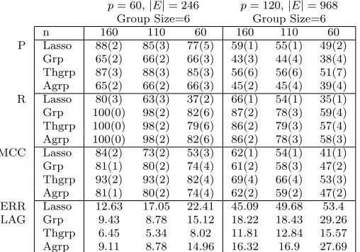
p= 60,|E|= 246 p= 120,|E|= 968 Group Size=6 Group Size=6
n 160 110 60 160 110 60
P Lasso 88(2) 85(3) 77(5) 59(1) 55(1) 49(2) Grp 65(2) 66(2) 66(3) 43(3) 44(4) 38(4) Thgrp 87(3) 88(3) 85(3) 56(6) 56(6) 51(7) Agrp 65(2) 66(2) 66(3) 45(2) 45(4) 39(4) R Lasso 80(3) 63(3) 37(2) 66(1) 54(1) 35(1) Grp 100(0) 98(2) 82(6) 87(2) 78(3) 59(4) Thgrp 100(0) 98(2) 79(6) 86(2) 79(3) 57(4) Agrp 100(0) 98(2) 82(6) 86(2) 78(3) 58(3) MCC Lasso 84(2) 73(2) 53(3) 62(1) 54(1) 41(1) Grp 81(1) 80(2) 74(4) 61(2) 58(3) 47(2) Thgrp 93(2) 93(2) 82(4) 69(4) 66(4) 53(3) Agrp 81(1) 80(2) 74(4) 62(2) 59(2) 47(2) ERR Lasso 12.63 17.05 22.41 45.09 49.68 53.4 LAG Grp 9.43 8.78 15.12 18.22 18.43 29.26
Thgrp 6.45 5.34 8.02 11.81 12.84 15.57 Agrp 9.11 8.78 14.96 16.32 16.9 27.69
Table 3: Performance of different regularization methods in estimating graphical Granger causality with misspecified groups (30% misspecification); d = 2, T = 10,
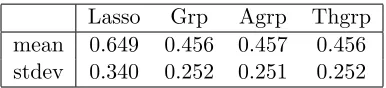
Lasso Grp Agrp Thgrp mean 0.649 0.456 0.457 0.456 stdev 0.340 0.252 0.251 0.252
Table 4: Mean and standard deviation of MSE for different NGC estimates
within group variable selection. We would like to mention here that a careful choice of the thresholding parametersδgrp and δmisspec via cross-validation improves the performance of thresholded group lasso; however, we do not pursue these methods here as they require grid search over many tuning parameters or an efficient estimator of the degree of freedom of group lasso.
In summary, the results clearly show that all variants of group lasso NGC outperform the lasso-based ones, whenever the grouping structure of the variables is known and correctly specified. Further, their performance depends on the composition of group sizes. On the other hand, if the a priori known group structure is moderately misspecified lasso estimates produce comparable results to regular and adaptive group NGC ones, while thresholded group estimates outperform all other methods, as expected.
6. Application
Example: T-cell activation. Estimation of gene regulatory networks from expression data is a fundamental problem in functional genomics (Friedman, 2004). Time course data coupled with NGC models are informationally rich enough for the task at hand. The data for this application come from Rangel et al. (2004), where expression patterns of genes involved in T-cell activation were studied with the goal of discovering regulatory mechanisms that govern them in response to external stimuli. Activated T-cells are involved in regulation of effector cells (e.g., B-cells) and play a central role in mediating immune response. The available data comprising ofn= 44 samples ofp= 58 genes, measure the cells response at 10 time points, t = 0,2,4,6,8,18,24,32,48,72 hours after their stimulation with a T-cell receptor independent activation mechanism. We concentrate on data from the first 5 time points, that correspond to early response mechanisms in the cells.
Genes are often grouped based on their function and activity patterns into biological pathways. Thus, the knowledge of gene functions and their membership in biological path-ways can be used as inherent grouping structures in the proposed group lasso estimates of NGC. Towards this, we used available biological knowledge to define groups of genes based on their biological function. Reliable information for biological functions were found from the literature for 38 genes, which were retained for further analysis. These 38 genes were grouped into 13 groups with the number of genes in different groups ranging from 1 to 5.
LASSO
API Apoptosis
cancer
cell cycle
cell differentiation cyclin
Jak−Stat signalling pathway
MAPK
Neurotrophin signalling pathway Osteoclast differentiation
T−cell receptor signalling pathway
TCF
Toll−like receptor signaling pathway API
Apoptosis
cancer
cell cycle
cell differentiation cyclin
Jak−Stat signalling pathway
MAPK
Neurotrophin signalling pathway Osteoclast differentiation
T−cell receptor signalling pathway
TCF
Toll−like receptor signaling pathway
THRESHOLDED GROUP LASSO
API Apoptosis
cancer
cell cycle
cell differentiation cyclin
Jak−Stat signalling pathway
MAPK
Neurotrophin signalling pathway Osteoclast differentiation
T−cell receptor signalling pathway
TCF
Toll−like receptor signaling pathway API
Apoptosis
cancer
cell cycle
cell differentiation cyclin
Jak−Stat signalling pathway
MAPK
Neurotrophin signalling pathway Osteoclast differentiation
T−cell receptor signalling pathway
TCF
Toll−like receptor signaling pathway
Figure 5: Estimated Gene Regulatory Networks of T-cell activation. Width of edges rep-resent the number of effects between two groups, and the network reprep-resents the aggregated regulatory network over 3 time points.
activated T-cells exhibit high levels of osteoclast-associated receptor activity which may attribute the large number of associations between member of osteoclast differentiation and other groups. Finally, the estimated networks based on variants of group lasso estimator also offer improved estimation accuracy in terms of mean squared error (MSE) despite having having comparable complexities to their regular lasso counterpart (Table 4), which further confirms the findings of other numerical studies in that paper.
depository institutions in U.S. foreign banks FRB
Noninterest−bearing
U.S. Government U.S. Treasury
states & political subdiv
Other domestic debt Private, residential mortgage
Foreign debt Equity
real estate loans
Farm loans
Commercial and industrial loans
Loans to individuals Interest income: Trading accounts
Interest income: Federal funds sold
deposit accounts (<= $250k) retirement deposit accounts (<= $250k)
deposit accounts (>$250k) retirement deposit accounts (> $250k) depository institutions in U.S.
foreign banks FRB Noninterest−bearing
U.S. Government U.S. Treasury
states & political subdiv
Other domestic debt Private, residential mortgage
Foreign debt Equity
real estate loans
Farm loans Commercial and industrial loans
Loans to individuals Interest income: Trading accounts
Interest income: Federal funds sold
deposit accounts (<= $250k) retirement deposit accounts (<= $250k)
deposit accounts (>$250k) retirement deposit accounts (> $250k) Balances due
Securities
Loans, Interest income
Deposit Amount
depository institutions in U.S. foreign banks FRB
Noninterest−bearing
U.S. Government U.S. Treasury states & political subdiv
Other domestic debt Private, residential mortgage
Foreign debt Equity
real estate loans
Farm loans
Commercial and industrial loans Loans to individuals Interest income: Trading accounts
Interest income: Federal funds sold
deposit accounts (<= $250k) retirement deposit accounts (<= $250k)
deposit accounts (>$250k) retirement deposit accounts (> $250k) depository institutions in U.S.
foreign banks FRB Noninterest−bearing
U.S. Government U.S. Treasury states & political subdiv
Other domestic debt Private, residential mortgage
Foreign debt Equity
real estate loans
Farm loans Commercial and industrial loans
Loans to individuals Interest income: Trading accounts
Interest income: Federal funds sold
deposit accounts (<= $250k) retirement deposit accounts (<= $250k)
deposit accounts (>$250k) retirement deposit accounts (> $250k) Balances due
Securities
Loans, Interest income
Deposit Amount
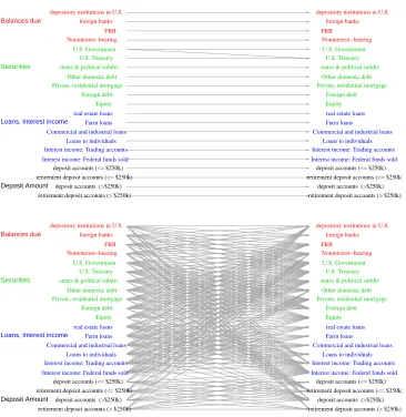
Figure 6: Estimated Networks of banking balance sheet variables using (a) lasso and (b) group lasso. The networks represent the aggregated network over 5 time points.
Quarter Lasso Grp Agrp Thgrp Dec 2010 1.59 (0.29) 0.36 (0.05) 0.36 (0.05) 0.37 (0.05) Mar 2011 1.46 (0.30) 0.47 (0.23) 0.47 (0.23) 0.46 (0.22) Jun 2011 1.33 (0.26) 0.36 (0.11) 0.36 (0.11) 0.35 (0.11) Sep 2011 1.72 (0.32) 0.50 (0.18) 0.50 (0.18) 0.47 (0.16)
Table 5: Mean and standard deviation (in parentheses) of PMSE (MSE in case of Dec 2010) for prediction of banking balance sheet variables.
The raw data are reported in thousands of dollars. The few missing values were imputed using a nearest neighbor imputation method with k = 5, by clustering them according to their total assets in the most recent quarter in the data collection period (September 2011) and subsequently every missing observation for a particular bank was imputed by the median observation on its five nearest neighbors. The data were log-transformed to reduce non-stationarity issues. The data set was restructured as a panel with p = 21 variables and
n= 50 replicates observed over T = 9 time points. Every column of replicates was scaled to have unit variance.
We applied the proposed variants of NGC estimates on the first T = 6 time points (Sep 2009 - Dec 2010) of the above panel data set. The parameters λ and δgrp were chosen
using a 19 : 1 sample-splitting method and the misspecification threshold δmisspec was set to zero as the grouping structure was reliable. We calculated the MSE of the fitted model in predicting the outcomes in the four quarters (December 2010 - September 2011). The Predicted MSE (MSE for Dec 2010) are listed in Table 5. The estimated network structures are shown in Figure 6.
It can be seen that the lasso estimates recover a very simple temporal structure amongst the variables; namely, that past values (in this case lag-1) influence present ones. Given the structure of the balance sheet of large banks, this is an anticipated result, since it can not be radically altered over a short time period due to business relationships and past com-mitments to customers of the bank. However, the (adaptive) group lasso estimates reveal a richer and more nuanced structure. Examining the fitted values of the adjacency matrices
At, we notice that the dominant effects remain those discovered by the lasso estimates. However, fairly strong effects are also estimated within each group, but also between the groups of the assets (loans and securities) on the balance sheet. This suggests rebalancing of the balance sheet for risk management purposes between relatively low risk securities and potentially more risky loans. Given the period covered by the data (post financial crisis starting in September 2009) when credit risk management became of paramount im-portance, the analysis picks up interesting patterns. On the other hand, significant fewer associations are discovered between the liabilities side of the balance sheet. Finally, there exist relationships between deposits and securities such as US Treasuries and other domestic ones (primarily municipal bonds); the latter indicates that an effort on behalf of the banks to manage the credit risk of their balance sheets, namely allocating to low risk assets as opposed to more risky loans.
thresholded estimates did not provide any additional benefits over the regular and adaptive variants, given that the specification of the groups was based on accounting principles and hence correctly structured.
7. Discussion
In this paper, the problem of estimating Network Granger Causal (NGC) models with in-herent grouping structure is studied when replicates are available. Norm, and both group level and within group variable selection consistency are established under fairly mild as-sumptions on the structure of the underlying time series. To achieve the second objective the novel concept of direction consistency is introduced.
The type of NGC models discussed in this study have wide applicability in different areas, including genomics and economics. However, in many contexts the availability of replicates at each time point is not feasible (e.g., in rate of returns for stocks or other macroeconomic variables), while grouping structure is still present (e.g., grouping of stocks according to industry sector). Hence, it is of interest to study the behavior of group lasso estimates in such a setting and address the technical challenges emanating from such a pure time series (dependent) data structure.
Acknowledgments
We thank the action editor and three anonymous reviewers for their helpful comments. The work of SB and GM was supported in part by DoD grant W81XWH-12-1-0130, and that of GM by NSF DMS-1106695 and NSA H98230-10-1-0203. The work of AS was partially supported by NSF grant DMS-1161565 and NIH grant 1R21GM101719-01A1.
Appendix A. Auxiliary Lemmas
Lemma A.1 (Characterization of the Group lasso estimate) A vector βˆ∈ Rp is a solution to the convex optimization problem
argmin
β∈Rp
1
2nkY −Xβk
2+
G
X
g=1
λgkβ[g]k (14)
if and only if βˆsatisfies, for some τ ∈Rp with max1≤g≤G
τ[g]
≤1, n1 h
X0(Y −Xβˆ)
i
[g]=
λgτ[g]∀g. Further, τ[g]=D
ˆ
β[g] whenever βˆ[g]6=0.
Proof Follows directly from the KKT conditions for the optimization problem (14).
Lemma A.2 (Concentration bound for multivariate Gaussian) LetZk×1∼N(0,Σ).
Then, for any t >0, the following inequalities hold:
P(|kZk −EkZk|> t)≤2 exp
− 2t
2
π2kΣk
, EkZk ≤
√
Proof The first inequality can be found in Ledoux and Talagrand (1991) (equation (3.2). To establish the second inequality note that,
EkZk ≤ q
EkZk2 = p
E[tr (ZZ0)] = p
tr (Σ)≤√kpkΣk.
Lemma A.3 Let β, βˆ∈Rm\{0}. Let uˆ= ˆβ−β and r = D( ˆβ)−D(β). Then krk <2δ whenever kuˆk< δkβk.
Proof It follows from kuˆk< δkβk that
(1−δ)kβk<kβk − kuˆk ≤ kβˆk ≤ kuˆk+kβk<(1 +δ)kβk,
which implies that
kβk − k ˆ
βk
< δkβk. Now,
kβˆk kβkkrk=
ˆ
βkβk+ (ˆu−βˆ)kβˆk ≤
ˆ
βkβk − kβˆk+kβˆk uˆ <k
ˆ
βk kβk(δ+δ),
since
kβk − k ˆ
βk
< δkβk andkuˆk< δkβk.
Lemma A.4 Let G1, . . . ,GG be any partition of {1, . . . , p} into G non-overlapping groups
andλ1, . . . , λGbe positive real numbers. Define the cone setsC(J, L) ={v∈Rp :Pg /∈Jλgkv[g]k
≤LP
g∈Jλgkv[g]k} for any subset of groups J ⊆NG. Also define the set of group s-sparse
vectors D(s) :={v∈Rp :kvk ≤1, supp(v)⊆ GJ for some J ⊆NG, |J| ≤s}. Then
[
J⊆NG,|J|≤s
C(J, L)∩Sp−1 ⊆(2 +L0)cl{conv{D(s)}}, (15)
where L0 =Lλmax/λmin, Sp−1 ={v∈ Rp :kvk = 1} is the ball of unit norm vectors in Rp
and cl{.}, conv{.} respectively denote the closure and convex hull of a set.
Proof Note that for any J ⊆NG,|J| ≤s, andv∈C(J, L)∩Sp−1, we have X
g /∈J
kv[g]k ≤Lλmax
λmin
X
g∈J
kv[g]k,
which implies
kvk2,1 ≤(L0+ 1) X
g∈J
kv[g]k ≤(L0+ 1)
√
skv[J]k ≤(L0+ 1)
√
s.
Hence the union of the cone sets on the left hand side of (15) is a subset of A:={v∈Rp:
kvk ≤1, kvk2,1 ≤(L0+ 1)
√
We will show that the set A is a subset of B := (2 +L0)cl{conv{D(s)}}, the closed convex hull on the right hand side of (15). Since both setsAand B are closed convex, it is enough to show that the support function ofA is dominated by the support function ofB. The support function of A is given by φA(z) = supθ∈Ahθ, zi. For any z ∈ Rp, let
S ⊆ {1, . . . , G}be a subset of topsgroups in terms of the`2norm ofz[g]. Thus,kz[Sc]k2,∞≤
kz[g]k for allg∈S. This implies kz[Sc]k2,∞≤(1/s)kz[S]k2,1 ≤(1/
√
s)kz[S]k. So, we have
φA(z) = sup
θ∈A
hθ, zi ≤ sup
kθ[S]k≤1
hθ[S], z[S]i+ sup
kθ[Sc]k2,1≤ √
s(L0+1)
hθ[Sc], z[Sc]i (16)
≤ kz[S]k+ (L0+ 1)
√
skz[Sc]k2,∞≤(L0+ 2)kz[S]k. (17)
On the other hand, support function ofB := (L0+ 2)cl{conv{D(s)}} is given by
φB(z) = sup θ∈B
hθ, zi= (L0+ 2) max
|U|=s, U⊆NG
sup
kθ[U]k≤1
hθ[U], z[U]i= (L0+ 2)kz[S]k.
This concludes the proof.
Lemma A.5 Consider a matrix Xn×p with rows independently distributed as N(0,Σ),
Λmin(Σ)> 0. Let G1, . . . ,GG be any partition of {1, . . . , p} into G non-overlapping groups
of size k1, . . . , kg, respectively. Let C =X0X/n denote the sample Gram matrix and D(s)
denote the set of groups-sparse vectors defined in Lemma A.4. Then, for any integers≥1
and any η >0, we have
P "
sup
v∈cl{conv{D(s)}}
|v0(C−Σ)v|>6ηkΣk
#
≤ c0exp
−nmin{η, η2}+c1s(kmax+c2log (eG/2s))
(18)
for some universal positive constants ci.
Proof We consider a fixed vectorv∈Rpwithkvk ≤1, the support of which can be covered by a set J of at most sgroups, i.e.,supp(v)⊆ GJ,J ⊆NG,|J| ≤s. DefineY =Xv. Then
each coordinate ofY is independently distributed asN(0, σ2y), whereσ2y =v0Σv≤ kΣk. Then, for any η > 0, Hanson-Wright inequality of Rudelson and Vershynin (2013) ensures
Pv0(C−Σ)v
> ηkΣk
≤P
1
n
Y0Y −EY0Y > ησ2y
≤2 exp
−cnmin{η, η2}
.
Next, we extend this deviation bound on all vectors v in the sparse set
D(2s) ={v∈Rp:kvk ≤1, supp(v)⊆ GJ for someJ ⊆NG, |J| ≤2s}. (19)
For a given J ⊆NG, |J|= 2s, we define DJ ={v ∈Rp :kvk ≤1, supp(v)⊆ GJ} and note
that D(2s) =∪|J|=2sDJ. For an >0 to be specified later, we construct an-netA of DJ.
Since P
We want a tail inequality for M := supv∈DJ|v0∆v|, where ∆ =C−Σ. Since A is an
-cover of DJ, for any v ∈DJ, there exists v0 ∈ A such that w =v−v0 satisfies kwk ≤ . Then
|v0∆v|=|(w+v0)0∆(w+v0)| ≤ |w0∆w|+|v00∆v0|+ 2|v00∆w|. Taking supremum over allv∈DJ, and noting thatw/∈DJ, we obtain
M ≤2M+ max
v0∈A
|v00∆v0|+ sup
u,v∈DJ
2|u0∆v|. (20)
To upper bound the third term, note that (u+v)/2∈DJ, and
2|u0∆v| ≤ |(u+v)0∆(u+v)|+|u0∆u|+|v0∆v|.
Hence
sup
u,v∈DJ
2|u0∆v| ≤4M+M+M= 6M.
From equation (20), we now have
M ≤(1−6−2)−1max
v0∈A
|v00∆v0|. Choosing >0 small enough so that (1−6−2)>1/2, we obtain
P "
sup
v∈DJ
|v0∆v|>2ηkΣk
#
≤ P
max
v0∈A
|v00∆v0|> ηkΣk
≤ 2 (1 + 2/)2s kmaxexp[−cnmin{η, η2}]. Taking supremum over
G
2s
≤(eG/2s)2s choices ofJ, we get
P "
sup
v∈D(2s)
|v0∆v|>2ηkΣk
#
≤2 exp
−cnmin{η, η2}+ 2slog
eG
2s
+ 2s kmaxlog
1 +2
.
In order to extend this deviation inequality to cl{conv{D(s)}}, we note that any v in the convex hull of D(s) can be expressed as v = Pmi=1αivi, where v1, . . . , vm are in D(s) and 0≤αi ≤1,
P
αi = 1. Then
|v0∆v| ≤
m
X
i=1
m
X
j=1
αiαj|v0i∆vj|.
Also, for every i, j, (vi+vj)/2∈D(2s), and
|v0i∆vj| ≤ 1
2
|(vi+vj)0∆(vi+vj)|+|v0i∆vi|+|vj0∆vj|
.
Hence
sup
v∈conv{D(s)}
|v0∆v| ≤
m
X
i=1
m
X
j=1
αiαj 1
2[4 + 1 + 1] supv∈D(2s)
Together with the continuity of quadratic forms, this implies
sup
v∈cl{conv{D(s)}}
|v0∆v| ≤3 sup
v∈D(2s)
|v0∆v|.
The result then readily follows from the above deviation inequality.
Appendix B. Proof of Main Results
Proof [Proof of Proposition 3.2] (a) Note that Σ is a p(T −1)×p(T−1) block Toeplitz matrix with (i, j)th block (Σij)1≤i,j≤(T−1) := Γ(i−j), where Γ(`)p×p is the autocovariance
function of lag`for the zero-mean VAR(d) process (2), defined as Γ(`) =E[Xt(Xt−`)0]. We consider the cross spectral density of the VAR(d) process (2)
f(θ) = 1
2π ∞
X
`=−∞
Γ(`)e−i`θ, θ∈[−π, π]. (21)
From standard results of spectral theory we know that Γ(`) =R−ππ ei`θf(θ)dθ, for every `. We want to find a lower bound on the minimum eigenvalue of Σ, i.e., infkxk=1x0Σx. Consider an arbitraryp(T−1)-variate unit norm vectorx, formed by stacking thep-tuples
x1, . . . , xT−1.
For every θ∈[−π, π], defineG(θ) =PT−1
t=1 xte−itθ and note that Z π
−π
G∗(θ)G(θ)dθ =
T−1 X
t=1
T−1 X
τ=1
(xt)0(xτ) Z π
−π
ei(t−τ)θdθ
=
T−1 X
t=1
T−1 X
τ=1
(xt)0(xτ) (2π1{t=τ}) = 2π T−1 X
t=1
(xt)0(xt) = 2π kxk2 = 2π.
Also let µ(θ) be the minimum eigenvalue of the Hermitian matrix f(θ). Following Parter (1961) we have the result
x0Σx =
T−1 X
t=1
T−1 X
τ=1
(xt)0Γ(t−τ)xτ =
T−1 X
t=1
T−1 X
τ=1 (xt)0
Z π
−π
ei(t−τ)θf(θ)dθ
xτ
= Z π
−π T−1 X
t=1
(xt)0eitθ
!
f(θ)
T−1 X
τ=1
xτe−iτ θ
!
dθ=
Z π
−π
G∗(θ)f(θ)G(θ)dθ
≥
Z π
−π
µ(θ) (G∗(θ)G(θ)) dθ ≥
min
θ∈(−π,π)µ(θ) Z π
−π
G∗(θ)G(θ)dθ= 2π min
θ∈(−π,π)µ(θ). So Λmin(Σ)≥2π min
θ∈(−π,π)µ(θ). Since
A(z) = I−A1z−A2z2−. . .−Adzd is the
(matrix-valued) characteristic polynomial of the VAR(d) model (2), we have the following represen-tation of the spectral density (see Priestley, 1981, eqn 9.4.23):
f(θ) = 1
2πσ
Thus, 2πµ(θ) = 2πΛmin(f(θ)) = 2π/Λmax(f(θ)−1) ≥ σ2/
A(e−iθ) 2
. But A(e−iθ)
≤
1 +Pd
t=1 At
for every θ ∈ [−π, π]. The result then follows at once from the standard matrix norm inequality (see e.g., Golub and Van Loan, 1996, Cor 2.3.2)
kAtk2 ≤pkAtk
1kAtk∞≤
kAtk1+kAtk∞
2 t= 1, . . . , d,
where
kAtk1= max 1≤i≤p
p
X
j=1
|Atij|, kAtk∞= max
1≤j≤p p
X
i=1
|Atij|.
(b) The first part of the proposition ensures that Λmin(Σ) ≥ σ2
1 +12(vin+vout)
−2 . If the replicates available from different panels are i.i.d, each row of the design matrix is independently and identically distributed according to a N(0,Σ) distribution.
To show that RE(s, L) of (5) holds with high probability for sufficiently large n, it is enough to show that
min
v∈C(J, L)\{0}
J ⊂NG¯, |J| ≤s
1
n
kXvk2
kvk2 ≥φ 2
RE (22)
holds with high probability, where the cone setsC(J, L) are defined as
C(J, L) :={v∈Rp¯:X
g /∈J
λgkv[g]k ≤L X
g∈J
λgkv[g]k} (23)
for all J ⊂NG¯ with|J| ≤s. Denote the ball of unit norm vectors inRp¯ by Sp−¯ 1. By scale invariance ofkXvk2/nkvk2, it is enough to show that with high probability
min
v∈Sp−¯ 1∩C(J, L)
J ⊂NG¯, |J| ≤s
v0Cv≥φ2RE, (24)
whereC =X0X/nis the sample Gram matrix.
By part (a), we already know that v0Σv ≥ Λmin(Σ) > 0 for all v ∈ Sp−¯ 1. So we only need to show that|v0(C−Σ)v| ≤Λmin(Σ)/2 with high probability, uniformly on the set
[
J⊆NG¯,|J|≤s
C(J, L)∩Sp−¯ 1. (25)
The proof relies on two key parts. In the first part, we use an extremal representation to show that the above union of the cone sets sits within the closed convex hull of a suitably defined set of groups-sparse vectors. In particular, it follows from Lemma A.4 that
[
J⊆NG¯,|J|≤s
C(J, L)∩Sp−¯ 1⊆(L0+ 2)cl{conv{D(s)}}, (26)
where D(s) = {v ∈ Rp¯ : kvk ≤ 1, supp(v) ⊆ GJ for some J ⊆ NG¯, |J| ≤ s}, L0 =
The next part of the proof is an upper bound on the tail probability of v0(C−Σ)v, uniformly over all v ∈ cl{conv{D(s)}}, presented in Lemma A.5. In particular, setting
η= Λmin(Σ)/12kΣk(2 +L0)2 in the above lemma yields
P "
sup
v∈(2+L0)cl{conv{
D(s)}}
|v0(C−Σ)v|>Λmin(Σ)/2 #
≤c0exp[−c1n] (27)
for the proposed choice ofn. Together with the lower bound on Λmin(Σ) established in part (a), this concludes the proof.
Proof [Proof of Theorem 4.1] Consider any solution ˆβR∈Rq of the restricted regression
argmin
β∈Rq
1 2n
Y−X(1)β 2 2+λ
s
X
g=1 β[g]
2 (28)
and set ˆβ = h
ˆ
βR0 :01×(p−q) i0
. We show that such an augmented vector ˆβ satisfies the statements of Theorem 4.1 with high probability.
Let ˆu= ˆβ(1)−β(1)0 = ˆβR−β0(1). In view of lemmas A.1 and A.3, it suffices to show that the following events happen with probability at least 1−4G1−α:
uˆ[g]
< δn
β
0 [g]
, for all g∈S, (29)
1 n
X0 −X(1)uˆ
[g]
≤λ, for all g /∈S. (30)
Note that, in view of Lemma A.1, ˆu = (C11)−1
1
√
nZ(1)−λτ
for some τ ∈ Rq with
τ[g]
≤1 for all g∈S, and Z = √1
nX
0=hZ0
(1) :Z
0
(2) i0
. Thus, for any g∈S,
P
uˆ[g]
> δn β 0 [g]
≤P
(C11)−1
1
√
nZ(1)−λτ
[g] > δn β 0 [g]
! ≤P h
(C11)−1Z(1) i
[g]
>√n
δn β 0 [g]
−λ h
(C11)−1τ i
[g] .
Note that V = (C11)−1Z(1) ∼N(0, σ2(C11)−1). So V[g] ∼N(0, σ2C [g][g]
11 ), where Σ[g][g] := (Σ−1)[g][g]. Also, by the second statement of lemma A.2 we haveEV[g]
≤σ p kg r C
[g][g] 11 . ThereforeP
uˆ[g]
> δn
β
0 [g]
is bounded above by
P V[g]
−E
V[g]
> √ n h δn β 0 [g]
−λ
(C11)
−1 √ s i −σ r kg C
[g][g] 11
!
≤2 exp "
− 2
π2σ2kC[g][g] 11 k
√
nδnkβ[0g]k −√nλkC11−1k√s−σ
q
kgkC11[g][g]k
2#