Random Intersection Trees

Random Intersection Trees

Rajen Dinesh Shah [email protected]

Statistical Laboratory University of Cambridge Cambridge, CB3 0WB, UK

Nicolai Meinshausen [email protected]

Seminar f¨ur Statistik ETH Z¨urich

8092 Z¨urich, Switzerland

Editor:John Lafferty

Abstract

Finding interactions between variables in large and high-dimensional data sets is often a serious computational challenge. Most approaches build up interaction sets incremen-tally, adding variables in a greedy fashion. The drawback is that potentially informative high-order interactions may be overlooked. Here, we propose an alternative approach for classification problems with binary predictor variables, called Random Intersection Trees. It works by starting with a maximal interaction that includes all variables, and then grad-ually removing variables if they fail to appear in randomly chosen observations of a class of interest. We show that informative interactions are retained with high probability, and the computational complexity of our procedure is of order pκ_{, where pis the number of}

pre-dictor variables. The value ofκcan reach values as low as 1 for very sparse data; in many more general settings, it will still beat the exponents obtained when using a brute force search constrained to ordersinteractions. In addition, by using some new ideas based on min-wise hash schemes, we are able to further reduce the computational cost. Interactions found by our algorithm can be used for predictive modelling in various forms, but they are also often of interest in their own right as useful characterisations of what distinguishes a certain class from others.

Keywords: high-dimensional classification, interactions, min-wise hashing, sparse data

1. Introduction

In this paper, we consider classification with high-dimensional binary predictors. We sup-pose we have data that can be written in the form (Yi, Xi) for observations i= 1, . . . , n;Yi

is the class label and Xi ⊆ {1, . . . , p} is the set of active predictors for observations i(out

of a total of p predictors). An important example of this type of problem is that of text classification, where then Xi is the set of frequently appearing words (in a suitable sense)

for document i, and Yi indicates whether the document belongs to a certain class. In this

Our aim here is to develop methodology that can discover important interaction terms in the data without requiring that any of their lower order interactions are also informative. More precisely, we are interested in finding subsets S⊆ {1, . . . , p} of all predictor variables that occur more often for observations in a class of interest than for other observations. We will use the terms “leaf nodes”, “rules”, “patterns” and “interactions” interchangeably to describe such subsetsS. For simplicity, suppose there are only two classes, the set of labels being{0,1}. The case with more than two classes can be dealt with using one-versus-one, or one-versus-all strategies. Given a pair of thresholds, 0≤θ0 < θ1 ≤1, our goal is to find all sets S (or as many as possible), for which

Pn(S⊆X|Y = 1)≥θ1 and Pn(S ⊆X|Y = 0)≤θ0. (1) Here and throughout the paper, we use the subscript n to indicate that the probabilities are empirical probabilities. For example, forc∈ {0,1},

Pn(S ⊆X|Y =c) :=

1

|Cc| X

i∈Cc

1{S⊆Xi},

where we have denoted the set of observations in class c by Cc. Of course, one would also

be interested in setsS which satisfy a version of (1) with classes 1 and 0 interchanged, but we will only consider (1) for simplicity.

The interaction terms uncovered can be used in various ways. For example, they can be built into tree-based methods, or form new features in linear or logistic regression models. The interactions may also be of interest in their own right, as they can characterise dis-tinctions between classes in a simple and interpretable way. These potentially high-order interactions that our method aims to target would be very difficult to discover using existing methods, as we now explain.

A pure brute force search examines each potential interactionS of a given size to check whether it fulfills (1). Restricting the order of interactions to size s, the computational complexity scales as ps, rendering problems with even moderate values ofp infeasible.

Instead of searching through every possible interaction, tree-based methods build up interactions incrementally. A typical tree classifier such as CART (Breiman et al., 1984) works by building a decision tree greedily from root node to the leaves; see also Loh and Shih (1997). The feature space is recursively partitioned based on the variable whose presence or absence best distinguishes the classes. The myopic nature of this strategy makes it a computationally feasible approach, even for very large problems. The downside is that it produces rather unstable results: small changes in the data can lead to very different partitions being produced at the leaf nodes. Moreover, because of the incremental way in which interactions are constructed, the success of this strategy in recovering an important interaction S rests on at least some of its lower order interactions being informative for distinguishing the classes.

complex and hard to interpret, one can examine what are known as variable importance measures. These aim to quantify the marginal or pairwise importance of predictor variables (Strobl et al., 2008). Though such measures can be useful, checking through all possible high-order interactions is too cumbersome, and so these may fail to be highlighted.

More recently, there has been interest in algorithms that start from deep splits or leaf nodes in trees and then try to build a simpler model out of many thousands of these leaves by regularisation and dimension reduction. Examples includeRule Ensembles (Friedman and Popescu, 2008),Node Harvest (Meinshausen, 2010) and the general framework ofDecision Lists (Marchand and Sokolova, 2006; Rivest, 1987). Though these methods have been demonstrated to improve onRandom Forests in some situations, they nevertheless crucially rely on a good initial basis of leaf nodes. These bases are usually generated by tree ensemble methods and so, if the base trees miss some important splits, they would also be absent in the results of these derivative algorithms.

A complementary approach has developed in data mining under the name of frequent itemset search, starting with the Apriori algorithm (Agrawal et al., 1994), which has since then developed into many improved and more specialised forms. The starting point for these was “market basket analysis”, where the shopping behaviour of customers is analysed and the goal is to identify items that are often bought together. Many algorithms have been proposed that aim to improve onApriori in terms of memory requirements and speed, such as the FP-growth (Han et al., 2000) and H-mine (Pei et al., 2001) algorithms. While generally very successful, all these methods are only computationally feasible in large-scale settings if among the itemsets of low size, there are many that are infrequent, and so using the principle that subsets of frequent itemsets are also frequent, the search space can be greatly reduced. However, if small itemsets all have roughly the same frequency, these methods cannot greatly improve over a brute force search.

We now give a simple example where tree-based approaches and those based on the

Apriori algorithm will struggle. LetZ = (Z1, . . . , Zp) ∈ {0,1}p be a random variable with

pindependent components each having a Bernoulli(1/2)-distribution. We take X to be the set of active entries {k :Zk = 1}. Suppose the response Y ∈ {0,1} is determined by an

interaction between the first two variables such that Y = 1{_Z1+Z26=1}. Then none of the

variables have a marginal effect as Y is independent ofZkfor all k= 1, . . . , p. In this case,

when using trees or theApriori algorithm, one would have to search amongO(p2) potential interactions to find the interaction pattern{1,2}.

This paper looks at a new way to discover interactions, which we call Random Inter-section Trees. Rather than searching through potential interactions directly, our method works by looking for collections of observations whose common active variables together form informative interactions. We present a basic version of theRandom Intersection Trees

2. Random Intersection Trees

Our method searches for important interactions by looking at intersections of randomly chosen observations from class 1. We start with the full set of variables as an interaction and then iteratively prune away variables to make the interaction smaller. At each iteration, we just keep variables in the interaction that are present in a new randomly chosen observation of class 1. All variables in the interaction that are not present in the chosen observation are removed. Then we repeat with a new randomly chosen observation until an interaction of the desired size emerges. If a patternS has high prevalence in class 1, that is,Pn(X =S|Y = 1)

is large, it will be included in the observations chosen with high probability. Thus, provided the overall process is repeated often enough, S is likely to be retained in some of the final intersections. On the other hand, elements in Sc, the complement of S in {1, . . . , p}, are unlikely to be present in all the observations being intersected. Thus of those intersections which containS, there is a good chance that at least one of them is exactlyS. Arranging the procedure in a tree-type search makes performing the intersections more computationally efficient; details are given in the following section. One would then consider each of these intersections as possible solutions of (1), checking whether their prevalence among class 0 is below θ0.

It may at first seem strange that in the above, class 0 plays a part in the procedure only at the very end. One might expect that many candidate interactions could be generated that have high prevalence in both classes 1 and 0 and thus would not be useful for distinguishing between classes. In Section 4, we do present an improved version of our algorithm that makes use of class 0 at an earlier stage. However, in the sparse setting we are considering here, interactions with high prevalence in either class would typically be rather few in number. Thus even if all interactions with high prevalence in class 1, and not necessarily low prevalence in class 0, were generated by the procedure outlined above, this would be a manageable number of candidate sets. Note that the assumptions that allow this to happen certainly do not trivialise the problem: even if, given all solutions to the first equation in (1), it is easy to uncover those interactions that additionally satisfy the second equation, the first part of the task is still very challenging.

To describe the details of our algorithm, we first define some terms associated with trees that will be needed later. Recall that a tree is a pair (N, E) of nodes and edges forming a connected acyclic (undirected) graph. We will always assume (with no loss of generality) that N ={1, . . . ,|N|}. Arooted tree is the directed acyclic graph obtained from a tree by designating one node as root and directing all edges away from this root.

Letα andβ be two nodes in a rooted tree, with β not the root node. If (α, β)∈E,β is said to be thechild ofα, andα, theparent ofβ. We will denote by ch(α), the set of children of a nodeα. Since we are only considering rooted trees here as opposed to general directed graphs, we will differ with convention slightly and will use pa(β) to mean the unique parent of β. Thus here, pa(β) is a node itself, whereas ch(α) is a set of nodes.

If α 6=β lies on the unique path from the root to β, we say α is an ancestor of β, and

number of ancestors of any particular node. Bylevel dof the tree, we will mean the set of nodes with depth d.

We will say an indexing of the nodes ischronological if, for every parent and child pair, larger indices are assigned to the child than the parent. In particular, the root node will be 1. Note that both depth-first and breadth-first indexing methods are chronological in this way.

Algorithm 1 A basic version of Random Intersection Trees for tree m= 1 to M do

Let m be a rooted tree of depth D, with each node j in levels 0, . . . , D−1 having

Bj children, where the Bj are i.i.d. with a pre-specified distribution. Denote by J the

total number of nodes in the tree, and index the nodes chronologically. For each of the nodesj= 1, . . . , J, let i(j) be an independently and uniformly chosen index in the set of class 1 observations{i:Yi= 1}.

SetS1 =Xi(1).

fornode j= 2 toJ do SetSj =Xi(j)∩Spa(j). end for

Denote the collection of resulting sets from all nodes at depth d, ford= 1, . . . , D, by

Ld,m={Sj : depth(j) =d}.

end for

return candidate set of interactionsLD :=SMm=1LD,m.

Algorithm 1 describes a basic version of theRandom Intersection Trees procedure. The reason for allowing random choices of children is for the proof of Theorem 1, where we can randomly choose the number of children to be in {b, b+ 1} for a suitable integer value b. Although we have allowed the number of children of each non-leaf node in the trees to be random, in practice we would take this as a fixed number.

Looking at the innermost for-loop, we see that each node in each tree is associated with a randomly drawn observation from class 1. For every tree, we visit each non-root node in turn, and compute the intersection of the observation assigned to it, and all those assigned to its ancestors. Because of the way the nodes are indexed, parents are always visited before their children, and this intersection can simply be computed asSj =Xi(j)∩Spa(j). This is crucial to reducing the computational complexity of the procedure, as we shall see in the next section.

Each of the sets assigned to the leaf nodes of each of the trees yields a collection of potential candidate interactions, LD. One could then proceed to test these as potential

solutions to (1); we present a more efficient approach in Section 4, where we build this testing step into the construction of the trees.

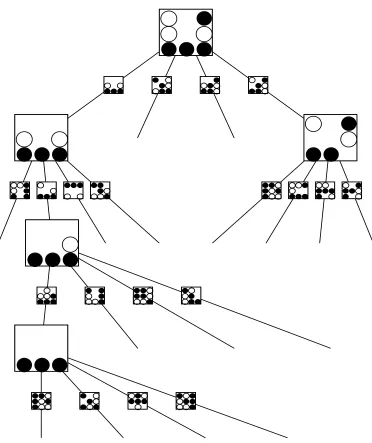
drawn final win-state for black (class 1). This corresponds toS1 in our algorithm. For each other node j, we draw a new random observation i(j) from all class 1 observations. The randomly chosen additional black-win state Xi(j) is shown along the edge from its parent node. The new intersection,Sj, is the intersection of the interaction in the parent node and

the new set Xi(j); it is shown in the corresponding node. The early stopping added in the improved algorithm also allows it to run until the algorithm has terminated in all nodes. Thus no prior specification of the tree depth will be necessary in practice, as will be shown in Section 4.

3. Computational Complexity

How many trees do we have to compute to have a very high probability of finding an interesting interactionSthat fulfills (1)? And what is the required size of these trees? If the interaction is not associated with a main effect, most approaches like trees and association rules would require of order p|S| searches. In this section, we show that in many settings,

Random Intersection Trees improves on this complexity. We consider a single interactionS

of sizes:=|S|, and examine the computational cost for returningS as one of the candidate interactions, with a given probability. We will see that this depends critically on three factors:

• Prevalence θ1 := Pn(S ⊆X|Y = 1) of the interaction pattern. If the pattern S in

question appears frequently in class 1, the search is more efficient.

• Sparsity δk:=Pn(k∈X|Y = 1) of the predictor variables k= 1, . . . , p. If δk is very

low for many k (and sparsity of predictors consequently high), computation of the intersections is much cheaper, and so overall computational cost is greatly reduced. Indeed, for a fixed tree m, consider a nodej with depth d < D. We have that

E(|Sj|) = p X

k=1

δd_k+1.

Thus, forj0∈ch(j), computation ofSj0 requires on average at most

O log(p)

p X

k=1

δ_kd+1

!

operations. This is because in order to compute the intersection, one can check whether each member ofSj is inXi(j0₎, and each such check isO(log(p)) if the setsX_i are ordered so a binary search can be used. If we compare this to the O(p) computa-tions required to calculate each of theSj if no tree structure were used, we see that

large efficiency gains are possible whend≥1 if many variables are sparse. For inter-sections with the root node, the tree structure offers no advantage, and in practice, branching the tree only after level 1 (so the root node has only one child), is more efficient, though this modification does not improve the order of complexity.

• Independence of S: Define ν := maxk∈Sc_Pn(k ∈ X|S ⊆ X, Y = 1). If ν is low,

●●●

● ● ●●

● ● ●●

● ● ●●

●

●●●

● ●

● ● ●●●

●●● ●●

● ●

●●●

●●

● ●

●

●

●●● ●●●●

● ●● ●

●

●●

● ●●●

● ●

● ●

●● ●● ●

● ● ●●

●●●

●●

● ●

●

● ●

● ●

●

●●● ●●●●

●

●●●

Figure 1: An intersection tree for the Tic-Tac-Toe game data set. Given winning positions of the black player, we intersect them randomly to produce the interactions (cor-responding to positions of black or white stones) that are responsible for wins. Starting with a randomly chosen class 1 (black wins) observation at the root node,B = 4 randomly chosen class 1 observations are intersected with the pat-tern. These randomly chosen observations are shown along the edges and the resulting intersections Sj as the nodes in the next layer of the tree. Nodes are

only shown if the corresponding patternsSj have an estimated prevalence among

class 0 below a set threshold; the branching of the tree terminates for all other nodes. The algorithm continues until all resulting Sj corresponding to the leaf

Pn(k∈X|S ⊆X) = 1, interest would centre onS∪ {k} rather thanS itself. Indeed,

if S satisfied (1), so wouldS ∪ {k}. In general, if ν is large, the search will tend to find sets containingS, though not necessarilyS itself.

With the assumptions that θ1 >0 and ν <1, we can give a bound on the computational complexity of the basic version of Random Intersection Trees introduced in the previous section.

Let us define

C(M, D, FB)

to be the expected number of computations required to perform all the intersections in the algorithm whenM trees of depth D are created and the distribution of the branching factorsBj isFB.

Theorem 1 Given η, ∈ (0,1], there exist choices of M, D and FB such that the set LD

returned by Algorithm 1 contains S with probability at least 1−η, and

C(M, D, FB) =O 

log(1/η)

log2(p)

p+ X

k: (1+)δk>θ1 p

log{(1+)_δk/θ1} log(1/ν)



. (2)

As a function of the number of variables p, there is a contribution of plog2(p) and an additional contribution in the brackets that depends on the sparsityδk of each variable.

Sparse variables do not contribute to this sum, which can beO(1) if sparsity among variables is high enough. This would yield a computational complexity with order bounded above by o(pκ) for any κ > 1, compared to the corresponding complexity of ps for a brute force search. In most interesting settings, however, we would not achieve a nearly linear scaling in complexity, but would hope to still be faster than a brute force search.

Before discussing the result further, we comment briefly on the values of M, Dand the distribution of theBj, that yield (2). From the proof, it follows that there exist choices of

M and Dgiving (2) that satisfy

M ≤ (1 + 2) log(1/η)

2θ1

,

D≤ log{p(1 + 2)}

log(1/ν) .

The random number Bj used in the proof takes just one of two consecutive integers

(es-sentially to avoid the discretisation effect when being restricted to integers), andE(Bj)≤

(1 +)/θ1. Though the optimal choices of parameters for the theorem depend on the un-knownν and the minimising, which will in turn depend onν, the functional relationships given above still provide rough qualitative guidelines for good choices for these parameters in practice.

Using the values ofM,Dand Bj necessary to guarantee that with high probabilityS is

in the setLD, we can also obtain a bound on the expected number of candidate interaction

expected number of sets returned is bounded by

E(|LD|)≤ME(Bj)D ≤

log(1/η)

(1 + 2)p ν

log(1+_log(1/ν)/θ₎1

.

The value of can be chosen to minimise the bound above, but its value here and in the computational complexity bound of Theorem 1 have to be the same, as they are linked to the choice of the branching factor used when building the trees. We see that in many situations, we can expect the bound above to be very much lower than the O(ps) sets a complete list of s-way interactions would contain. Note that ifswere known, the relevant quantity to consider would be

E(|{S0∈LD :|S0|=s}|),

which is likely to be much less than E(|LD|). Even ifs were unknown, one would only be

interested in the expected number of non-empty sets inLD, a quantity which may well also

be substantially lower than the derived bound onE(|LD|).

3.1 The Influence of Sparsity on Computational Complexity

It is interesting to make the influence of the sparsity of individual variables,δk, on the overall

computational complexity, more explicit. We have the following corollary to Theorem 1.

Corollary 2 Define β by ν =θβ₁. Suppose that γ, α?_{, α}

? are such that α? > α?, and

δk ≤ θ1−α ?

1 for allk∈ {1, . . . , p},

δk > θ11−α? for at most pγ variables.

Given η ∈ (0,1], there exist choices of M, D and FB such that the set LD returned by

Algorithm 1 contains S with probability at least 1−η, and

C(M, D, FB) =o pκ

for anyκ >max

α? β +γ,

hα_?

β

i

++ 1

.

The implication of Corollary 2 is most apparent if we takeγ = 1 as we can then setα? = 0.

In this case,

α?= 1−log(maxkδk)

log(θ1) .

We can then bound the computational complexity by

o pκ

for any κ >1 +log(1/θ1)−log(1/maxkδk) log(1/ν) .

The fraction on the right-hand side is a function of the prevalence of the pattern S, θ1, the maximum sparsity of the variables, and the maximum sparsity of the variables in Sc, conditional on the presence of S. As long as this fraction is less than 1, the computational complexity is guaranteed to be better than a brute force search with the knowledge that

3.2 Independent Noise Variables

To gain further insight, we consider the special case where variables in Sc_{are independent}

of S (conditional on being in class 1), in the sense that for allk∈Sc,

Pn(k∈X|S⊆X, Y = 1) =Pn(k∈X|Y = 1) =δk. (3)

Corollary 3 Assume (3)and that δk<1 for allk. Givenη ∈(0,1], there exist choices of

M, D and FB such that the set LD returned by Algorithm 1 contains S with probability at

least 1−η, and

C(M, D, FB) =o(pκ) for any κ >

log(1/θ1) log(1/maxkδk)

. (4)

We see that the computational complexity is approximately linear inp if the prevalence of the pattern S is as high as the prevalence of the least sparse predictor variables. This is the case in the example mentioned in the introduction, where θ=δk= 1/2.

We can also consider the situation where in addition to the independence (3), all vari-ables have the same sparsityδ. If the prevalenceθ1 ofSis only as high as that of a random occurrence of two independent predictor variables, we get κ > 2 and the computational complexity is approximately quadratic in p. In this case, the algorithm would not yield a computational advantage over brute force search if looking for patterns of size 2. This is to be expected sinceevery patternS of size 2 would have the same prevalence in this scenario, and so there is nothing special about a patternS of size 2 with prevalenceδ2, and in general no hope of beating the complexity ps of a brute force search. However, the bound in (4) is independent of s. Thus provided the prevalence, θ1, drops more slowly than the rate δs, at which every pattern of size S would occur randomly among independent predictor variables, our results show that Random Intersection Trees is still to be preferred over a brute force search.

4. Early Stopping Using Min-Wise Hashing

While Algorithm 1 is computationally attractive, the following observation suggests that further improvements are possible. Suppose that, for a particular tree, we have just com-puted the intersectionSj corresponding to a node j at depthd < D. If

Pn(Sj ⊆X|Y = 0)> θ0, then since for allj0 ∈de(j), Sj0 ⊆S_j, we also have

Pn(Sj0 ⊆X|Y = 0)> θ₀.

Thus no intersection sets corresponding to descendants of j have any hope of yielding solutions to (1), and so all further associated computations are wasted.

In view of this, one option would be to compute the quantity Pn(Sj ⊆ X|Y = 0) at

descendantsj0 of j for computation ofSj0. This could be prohibitively costly, though, as it would require a pass over all observations in class 0, for each node of each tree. One could work with a subsample of the observations, but if θ0 is low, the subsample size may need to be fairly large in order to estimate the probabilities to a sufficient degree of accuracy.

Instead, we propose a fast approximation, using some ideas based on min-wise hashing (Broder et al., 1998; Cohen et al., 2001; Datar and Muthukrishnan, 2002) applied to the columns of the data-matrix. We describe the scheme by leaving aside the conditioning on

Y = 0, which can be added at the end by restricting to observations in class 0. Consider taking a random permutation σ of all observations {1, . . . , n}. Let hσ(k) be the minimal

valueι such that variablek is active in observation σ(ι):

hσ(k) := min{ι0:k∈Xσ(ι0₎}.

It is well known (Broder et al., 1998) that the probability that hσ(k) and hσ(k0) agree for

two variables k, k0 under a random permutation σ is identical to the Jaccard-index for the two sets Ik={i:k∈Xi}and Ik0 ={i:k0 ∈X_i}, that is

Pσ(hσ(k) =hσ(k0)) =

|Ik∩Ik0|

|Ik∪Ik0|.

Here the subscriptσindicates that the probability is with respect to a random permutation

σ of the observations. A min-wise hash scheme is typically used to estimate the Jaccard-index by approximating the probability on the left-hand side of the equation above.

Now,

Pn(S ⊆X) =Pn(k∈X for all k∈S)

=Pn(k∈X for all k∈S| ∃k0 ∈S such thatk0 ∈X) ×_Pn(∃k∈S such thatk∈X).

Let us denote the first and second terms on the right-hand side byπ1(S) andπ2(S) respec-tively. Note that π1(S) is equal to the probability that all variables k ∈S have the same min-wise hash value hσ(k):

π1(S) =Pσ(∃ι:hσ(k) =ιfor all k∈S). (5)

Turning now to π2(S), observe that Eσ(min

k∈Shσ(k)) =

n+ 1

π2(S)n+ 1

, (6)

and so

π2(S) = n+ 1

n

1

Eσ(mink∈Shσ(k))

− 1

n+ 1

. (7)

A derivation of (6) is given in the appendix.

Equations (5) and (7) provide the basis for an estimator ofPn(S⊆X). First we generate

L random permutations of {1, . . . , n}: σ1, . . . , σL. We then use these to create an L×p

matrixH whose entries are given by

Now we estimate π1(S) and π2(S) by their respective finite-sample approximations, ˆπ1(S) and ˆπ2(S):

ˆ

π1(L;S, H) := _L1

L X

l=1

1{Hlk=H_lk0 for allk,k0∈S},

ˆ

π2(L;S, H) := n+ 1

n

(

1 1

L PL

l=1mink∈SHlk

− 1

n+ 1

)

.

Finally, we estimate Pn(S ⊆X) by

ˆ

Pn(L;S, H) := ˆπ1(L;S, H)·πˆ2(L;S, H). (8) To our knowledge, this use of min-wise hashing techniques, and in particular the estimator ˆ

π2(L;S, H), is new. The estimator enjoys reduced variance compared to that which would be obtained using subsampling, as the following theorem shows.

Theorem 4 ForPˆn(L;S, H),π1(S) and π2(S) defined as in (8), (5), and (7) respectively,

as L→ ∞, we have

√

L(ˆPn(L;S, H)−Pn(S ⊆X)) d

→N(0, π2(S)2π1(S)(1−π1(S)π2(S))(1 +(n))), (9)

where

(n) = 1

n

n−1−π₂2−2π2n−1 π2(π2+ 2n−1)(1 +n−1)

=O(n−1). (10) A derivation is given in the appendix. If we tried to estimate π1π2 by evaluating the prevalence ofS on a subset of the data of sizeL, the corresponding estimator multiplied by

√

Lwould have variance

π2(S)π1(S)(1−π1(S)π2(S)) +on(1),

where on(1) → 0 as n → ∞. Comparing this variance to the variance of the normal

distribution in (9), we see that a factor of π2(S) is gained: matching the accuracy of the min-wise hash scheme with subsampling would require roughly 1/π2(S) times as many samples. By using min-wise hashing, choosing L = 100 typically delivers a reasonable approximation as long as we just want to resolve values at θ0 = 0.01 and above.

An improved version of Algorithm 1, building in the ideas discussed above, is given in Algorithm 2 below. Note that ˆPn(Spa(j), H) need only be computed once for every j with the same parent.

Early stopping decreases the computational cost of the algorithm as many nodes in the trees generated may not need to have their associated intersections calculated. In addition, the set of candidate intersectionsLD will be smaller but the chance of it containing

Algorithm 2 Random Intersection Trees with early stopping

Compute theL×pmin-wise hash matrix H, using only class 0 observations. for tree m= 1 to M do

Let m be a rooted tree of depth D, with each node j in levels 0, . . . , D−1 having

Bj children, where the Bj are i.i.d. with a pre-specified distribution. Denote by J the

total number of nodes in the tree, and index the nodes chronologically. For each of the nodesj= 1, . . . , J, let i(j) be an independently and uniformly chosen index in the set of class 1 observations{i:Yi= 1}.

SetS1 =Xi(1).

fornode j= 2 toJ do if Pˆn(Spa(j), H)≤θ0 then

Set Sj =Xi(j)∩Spa(j). end if

end for

Denote the collection of resulting sets of all nodes at depth d, ford= 1, . . . , D, by

Ld,m={Sj : depth(j) =d}.

end for return LD :=

SM

m=1LD,m.

Trees with early stopping in all the practical examples to follow, taking small values of L

in the range of a (few) hundred permutations.

The depth D of the tree is still given explicitly in Algorithm 2. An interesting modifi-cation creates the tree recursively. Starting with the root node,B children are added to all leaf nodes of the tree in which the early stopping criterion has not been triggered yet. When the algorithm terminates, all intersections in the leaf nodes of the final tree are collected.

5. Numerical Examples

In this section, we give two numerical examples to provide further insight into the per-formance of our method. The first is about learning the winning combinations for the well-known game Tic-Tac-Toe. This example serves to illustrate howRandom Intersection Trees can succeed in finding interesting interactions when other methods fail. The second example concerns text classification. Specifically, we want to find simple characterisations (using only a few words, or word-stems in this case) for classes within a large corpus in a large-scale text analysis application.

5.1 Tic-Tac-Toe Endgame Prediction

0

10

20

30

40

50

RI RF RF3

TREE

TREE3

1−NN 3−NN 5−NN 10−NN RI RF RF3

TREE

TREE3

1−NN

3−NN

5−NN

10−NN

RI

RF RF3

TREE

TREE3

1−NN

3−NN

5−NN

10−NN

RI

RF

RF3

TREE

TREE3

1−NN

3−NN

5−NN

10−NN

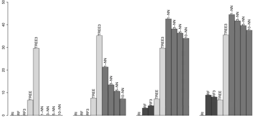
Figure 3: From left to right: the misclassification rate (in %) on Tic-Tac-Toe data for 0, 60, 300 and 400 added noise variables. Each classifier is tuned to have equal misclassification rate in both classes. The simple classifier based on Random Intersection Trees (RI) has a misclassification rate of 0% in all cases, as the winning patterns are sampled very frequently (see Figure 2). Random Forests

(RF) andRandom Forestslimited to depth 3 trees (RF3) are competitive but the misclassification rate increases sharply when many noise variables are added.

There are 9 variables in the original data set which can take the values ‘black’, ‘white’ or ‘blank’. These can trivially be transformed into a set of twice as many binary variables where the first block of variables encodes presence of black and the second block encodes presence of white.

Two properties of this data set that make it particularly interesting for us here are:

• The presence of interactions is obvious by the nature of the game.

• There are only very weak marginal effects. Knowing that the upper right corner is occupied by a black stone is only very weakly informative about the winner of the game. Greedy searches by trees fail in the presence of many added noise variables and linear models do not work well at all.

Figure 2 illustrates the importance sampling effect of Random Intersection Trees when using only the training data, and adding a varying number of noise variables. When adding 100 noise variables, all 16 winning final combinations are among the 40 most frequently chosen patterns. All winning states are chosen hundreds of millions times more often than a random sampling of interactions would pick them.

As discussed in Section 1, the interactions or rules that are found could be entered into any existing aggregation method, such as Rule Ensembles (Friedman and Popescu, 2008) or Decision Lists (Marchand and Sokolova, 2006; Rivest, 1987). Here, we consider an even simpler aggregation method by selecting all patterns during 1000 iterations of

Random Intersection Trees (withB= 5 samples as branching factor in each tree) that were selected by at least two trees. For each selected pattern, we compute the (empirical) class distributions conditional on the presence and absence of the pattern, using the training sample. That is, for each selected patternS, we compute

Pn(Y = 1|X⊆S) and Pn(Y = 1|X *S).

Then, given an observation from the test set, we classify according to the average of the log-odds of being in class 1 calculated from each of the conditional probabilities above.

Figure 3 shows the misclassification rates under situations with different numbers of added noise variables. The simple prediction based onRandom Intersection Trees achieves perfect classification even when 400 noise variables are added. Neither k-NN nor CART

(Breiman et al., 1984), either restricted to trees of depth 3 (TREE3) or depth chosen by cross-validation (TREE), are as successful, giving misclassification rates between 5% and 40%. Interestingly, trees of depth 3 perform much worse than deeper trees. The winning patterns are not identified in a pure form but only after some other variables have been factored in first. This also means that it is very hard to read the winning states of the trees, unlike the patterns obtained by our method. Random Forests also maintain a 0% misclassification rate up until about a hundred added noise variables but start to degrade in performance when further noise variables are added. It is easy to identify the noise variables from a variable importance plot (Strobl et al., 2008). However, within the signal variables the patterns are not easy to see since each variable is approximately equally important for determining the winner (with the slight exception of the middle field in the 3×3 board which is more important than the other fields) and the nature of the interactions is thus not obvious from analysing a Random Forest fit.

5.2 Reuters RCV1 Text Classification

The Reuters RCV1 text data contain the tf-idf (term frequency-inverse document fre-quency) weighted presence of 47,148 word-stems in each document; for details on the collection and processing of the original data, see Lewis et al. (2004). Each document is assigned possibly more than one topic. Here we are interested in whether Random Inter-section Trees is able to give a quick and accurate summary of each topic. For each topic, we seek sets of word-stems,S, whose simultaneous presence is indicative of a document falling within that topic.

0.00 0.25 0.50 0.75 1.00

0.00 0.25 0.50 0.75 1.00

● ●● ● ●● ● ●● ● ●● ● ●● ● ● ● ● ●● ● ● ● ● ●● ● ●● ● ● ● ● ●● ● ●● ● ●● ● ●● ● ●● ● ●● ● ● ● ● ● ● ● ● ● ● ●● ● ● ● ● ●● ● ●● ● ●● ● ●● ● ●● ● ●● ●●● ● ● ● ● ●● ● ●● ● ●● ● ● ● ● ●● ● ● ● ● ● ● ● ●● ● ●● ● ●● ● ●● ● ●● ● ● ● ● ●● ● ● ● ● ● ● ● ●● ● ●● ● ● ● ● ●● ● ● ● ● ●● E11 ECAT M11 M12 MCAT C24 CCAT C151 C15 E41 GCAT GJOB C11 M14 M132 M13 C12 GCRIM C13 C31 C42 E12 M131 C181 C18 GPOL M143 E512 E51 G15 GDIP GVOTE C152 C21 M142 C33 C17 E211 E21 GVIO C174 E212 C1511 C411 C41 C183 M141 C172 C171 GSPO GDIS GDEF

coupon / date / deliv / tax coupon / date / deliv / sery usda / week

alert / rate / research note / profit / shr note / shr goal / socc

market / sulphur / trad friday / index / shar / volum index / point / stock / trad chief / name / newsdesk / offic end / incom / net / q4 chief / name / newsdesk futur / ton / trad ballot / elect / poll / vote govern / milit offer / shar / underwrit net / profit

announc / issu / moody / rate currenc / interbank / newsroom / trad alumin / cop / lead

demo / polit / vote dollar / interbank area / flood / peopl / rain capit / fight / rebel bln / bond / lead / typ aa / issu / rate / stat charg / prosecut auction / bill / day compan / court / file / suit negot / strik / union / work assembl / countr / stat / test econom / gdp

talk / union / wag / work compan / merg / sharehold merg / sharehold deficit / revenu / spend brussel / european / plan / union commit / iraq / stat / unit basi / bond / treasur / yield gdp / growth / pct / percent tariff / told / trad

aver / crop / percent contract / win / won billion / deficit / export / import strik / told / tuesday / work form / joint / ventur shut / unit

currenc / monet / told banc / bank / govern / minist regulat / requir

percent / period / ton / year

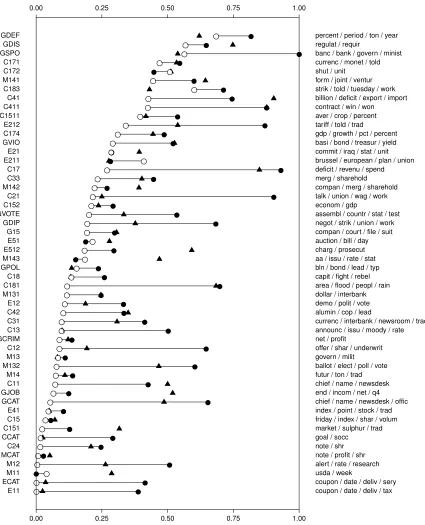
Figure 4: The misclassification rate Pn(c /∈ Y|S ⊆ X) on the test data for a pattern S

chosen with a tree ensemble node generation mechanism (black circles),Random Intersection Trees(white circles), and a linear method (black triangles) for topics

following 30000 documents as test documents. We compare our procedure to an approach based onRandom Forests and a simple linear method.

Random Forests and classification trees can be very time- and memory-intensive to apply on a data set of the scale we consider here. In order to be able to computeRandom Forests, we only consider word-stems if they appear in at least 100 documents in the training data. This leaves 2484 word-stems as predictor variables. We also only consider topics that contain at least 200 documents. To simplify the problem further, we consider a binary version of the predictor variables for all methods, using a 1 or 0 to represent whether each tf-idf value is positive or not.

Let C be the set of topics in our modified data set. Let Y ⊆C indicate the topics that a given document belongs to. Consider a topic or class c∈C. Our goal is to find patterns

S that maximise

Pn(c∈Y|S⊆X), (11)

whilst also maintaining that the prevalence of S among all observations be bounded away from 0. Specifically, we shall require that

Pn(S ⊆X)≥pc/10 wherepc=Pn(c∈Y). (12)

To see how this can be cast within the framework set in (1), note that ifS? maximises (11) and S?? satisfies

Pn(S??⊆X|Y ∈c)≥Pn(S?⊆X|Y ∈c) and

Pn(S??⊆X|Y /∈c)≤Pn(S?⊆X|Y /∈c),

then

Pn(c∈Y|S? ⊆X) = Pn

(S?⊆X|c∈Y)Pn(c∈Y)

Pn(S?⊆X|c∈Y)Pn(c∈Y) +Pn(S?⊆X|c /∈Y)Pn(c /∈Y)

≤ Pn(S

??_⊆X|c∈Y)

Pn(c∈Y)

Pn(S??⊆X|c∈Y)Pn(c∈Y) +Pn(S??⊆X|c /∈Y)Pn(c /∈Y)

=Pn(c∈Y|S??⊆X),

whence S?? also maximises (11) by optimality of S?. Thus treating those documents be-longing to topicc as class 1, and all others as class 0, by solving (1) withθ0 and θ1 chosen appropriately, we can obtain all solutions to (11).

In view of this, we use each of the methods to search for patterns S that have high prevalence for a given topic c. We then remove all patterns that do not satisfy (12) on the test data. Then, from the remaining patterns, we select the one that maximises (11) on training data. Below, we describe specific implementation details of each of the methods under consideration.

To computeRandom Intersection Trees, we create the min-wise hash table for the preva-lence among all samples once, using 200 permutations with associated min-wise hash values for each word-stem. Then 1000 iterations of the tree search are performed with a cut-off valueθ0 = (3/20)pc and all remaining patterns S with a length less than or equal to 4 are

For a tree-based procedure, one approach is to fit classification trees on subsampled data and adding randomness in the variable selection as in Random Forests (Breiman, 2001) and then looking among all created leaf nodes for the most suitable node among all nodes created.

We generate 100 trees as in the Random Forests method: each is fit to subsampled training data using CART algorithm restricted to depth 4, and further randomness is injected by only permitting variables to be selected from a random subset of those available, for each tree. This takes on average between 90% to 110% of the computational time of a non-optimised pure R (R Core Team, 2013) implementation ofRandom Intersection Trees

for these data. Note that this is when using the Fortran version of Breiman (2001) for the

Random Forests node generation; we expect a significant speedup if Fortran or C code were used for Random Intersection Trees. We are currently working on such a version and plan to make it available soon. Furthermore, Random Forests would scale much worse if many more word-stems were included as variables.

For linear models, we fit a sparse model with at most `predictors (with`≤4), using a logistic model with an `1-penalty (Tibshirani, 1996; Friedman et al., 2010). We constrain the regression coefficients to be positive since we are only looking for positive associations in the two previously discussed approaches, and want to keep the same interpretability for the linear model. For each value of ` ≤ 4, we take S` to be the set of variables with a

positive regression coefficient. We select the largest value of ` such that the fraction of documents attaining the maximal value is at least pc/10 and select the associated pattern

S`. (An alternative approach would be to retain the documents with the highest predicted

value when using a sparse regression fit. This approach gave very similar results.)

After screening the candidate patterns returned by each of the methods using (12) on all of the topics c∈C, we evaluate the misclassification rate Pn(c /∈Y|S ⊆X) on the test

data. The results for all of the topics are shown in Figure 4. The rules found withRandom Intersection Trees have a smaller loss than those found withRandom Forests in all but 5 of the topics. For those topics where Random Forests performs better, the difference in loss is typically small. Linear models achieve a smaller loss than Random Forests among most of the topics, but only have a smaller loss thanRandom Intersection Treesin 6 topics, performing worse in all remaining 46 topics.

6. Discussion

our complexity bound typically has a smaller exponent than that for a brute force search. Further improvements can be made by using min-wise hashing techniques to terminate parts of the search (i.e., branches of the Intersection Tree) that have no chance of leading to interesting interactions. Numerical examples illustrate the improved interaction detection power ofRandom Intersection Trees over other tree-based methods and linear models.

There are many diverse ways in which interactions that solve (1) can be used in further analysis. The interactions may be of interest in their own right as shown in both numerical examples. One can also simply use the search to make sure that a data set is unlikely to have strong interactions that could otherwise have been missed. If the aim is to build a classifier, they can be added to a linear model, or built into classifiers based on tree ensembles. For the latter approach one could consider, for example, averaging predictions in a linear way or averaging log-odds as in Random Ferns (Bosch et al., 2007). We believe developments along these lines will prove to be fruitful directions for future research. We also plan to generalise the idea to categorical and continuous predictor variables.

Appendix A.

Here we include proofs omitted earlier in the paper.

Proof of Theorem 1. Fix a tree m ∈ {1, . . . , M} and suppose this has node set N =

{1, . . . , J} indexed chronologically (see Section 2). Ford∈ {1, . . . , D}, define

Nd={j ∈N : depth(j) =dandSj ⊇S},

Wd=|Nd|.

Let E be the event that S is contained in S1, the random sample selected for the root node of treem. Further, let Gd(t) = E(tWd|E), the probability generating function of Wd

conditional on the event E.

We make a few simple observations from the theory of branching processes. Firstly, for

d≤D−1, Gd+1=Gd◦G whereG:=G1. To see this, first note that Wd+1=

X

j∈Nd

X

j0_∈ch(j)

1{S⊆X_i(j0₎}.

Now conditional on E, the random variablesP

j0_∈ch(j)1{_S⊆X

i(j0)} forj ∈Nd, are indepen-dent of Nd. Moreover, they are independent of each other and have identical distributions

equal to that of

X

j0_∈ch(1)

1{S⊆X_i(j0₎}=W1.

This entails

E(tWd+1|Wd=w, E) ={E(tW1|E)}w ={G(t)}w. Thus

Gd+1(t) =E(E(tWd+1|Wd, E)|E) =E({G(t)}Wd|E) =Gd(G(t)),

as claimed.

and q0∈(0,1], thenGd(q0)≤q. The relevance of these remarks will become clear from the

following: for anS0 ∈LD,m, we have

GD(P(S0 )S|S0 ⊇S)) =

∞ X

`=0

P(WD =`|E)P(S0 )S|S0 ⊇S)`

=

∞ X

`=0

P({WD =`} ∩ {S /∈LD,m}|E)

=P(S /∈LD,m|E).

Thus if we can ensure that P(S0 ) S|S0 ⊇ S) is at most q, then the final probability in the above display will also be at most q. The rest of the proof proceeds with the following steps:

1. Find conditions onFB, the distribution of theBj, such that there exists a fixed point

of G,q.

2. Find conditions on the tree depthD such thatP(S0 )S|S0 ⊇S)≤q.

3. Givenq establish conditions onM such that the overall probability of recoveringS is at least 1−η.

4. GivenFB,Dand M, compute the expected computational cost of the algorithm.

Step 1: Let the distribution of the Bj be such that

Bj = (

b with probability 1−α,

b+ 1 with probability α.

Now given aq∈(0,1], we shall pickb∈_Z+ and α∈[0,1) to satisfy G(q) =q. To this end, observe that

G(q) = (1−α)(1−θ1(1−q))b+α(1−θ1(1−q))b+1

= [1− {(α+b)− bα+bc}θ1(1−q)]{1−θ1(1−q)}bα+bc.

From the last displayed equation, we see thatG(q) varies withα+bcontinuously. Further-more, whenα+b= 0, G(q) = 1, and by makingα+blarge, we can make G(q) arbitrarily close to 0. Thus by the intermediate value theorem, for anyq ∈(0,1], α+b can be chosen such thatG(q) =q.

We now bound α+b from above in terms of q for use later in creating a bound on the complexity of the algorithm. We have

b+α= log(q)−log(1−αθ1(1−q)) log(1−θ1(1−q))

+α

≤ −log(q) + log(1−αθ1(1−q))

θ1(1−q)

+α

≤ −log(q)

θ1(1−q)

≤ 1 + (1−q)/(2q)

θ1

In the final line, we used the inequality

log(z)≥(z−1)−(z−1)

2

2z , 0< z≤1.

Step 2: We now boundP(S0 )S|S0 ⊇S) from above in terms ofD. The set S0 is the intersection ofD+ 1 observations selected independently of one another. In order for some

k ∈ Sc to be contained in S0, it must have been present in all these D+ 1 observations. Thus by the union bound we have

P(S0 )S|S0⊇S) ≤

X

k∈Sc

P(k∈S0|S0 ⊇S) ≤ pνD+1,

the rightmost inequality following from (A2). To ensure this is at most q, we take

D=

log(p/q) log(1/ν)

−1, (14)

so

D≤ log(p/q)

log(1/ν). (15)

Step 3: Turning now to the probability of recovering S, we have

P(S ∈LD) = 1−[1− {1−P(S /∈LD,m|E)}θ1]M.

Given the choices of α and b (13), and D (14), we have that P(S /∈ LD,m|E) ≤ q. Thus

takingM to be at least

−log(η) (1−q)θ1

≥ −log(η)

log{1−(1−q)θ1}

(16)

guarantees recovery of S with probability at least 1−η.

Step 4: To bound the complexity of the algorithm, observe that E(Bj) =b+α, so

C(M, D, FB)≤log(p)M p X

k=1

[(b+α)δk+· · ·+{(b+α)δk}D]

≤log(p)M D

p+ X

k:(b+α)δk>1

(b+α)δk D

−1

. (17)

Substituting Equations (13), (15) and (16) into the complexity bound (17), and writing

= (1−q)/(2q) gives a bound for the computational complexity of

log(p)log(1/η)

θ1

1 + 2

2

log{p(1 + 2)}

log(1/ν)

p+ X

k:(1+)δk>θ1

p(1 + 2)

log{(1+)_δk/θ1} log(1/ν) ₋₁

. (18)

log(1/η)log 2_(p)

p+ X

k:(1+)δk>θ1

p

log{(1+)_δk/θ1} log(1/ν) ₋₁

.

Proof of Corollary 2. Note that

X

k:(1+)δk>θ1

p

log((1+)_δk/θ1) log(1/ν)

is bounded by

(1 +) log(p) log(1/ν)

pγ·pα?/β1{α?_/β>0} + p·pα?/β1{_α?/β>0}

.

The result then follows from substituting into (18) and taking∝1/log(p)

Proof of Equation (6). Writingr =nπ2(S), we have

n r

Eσ(min

k∈Shσ(k)) =

n−r+1

X

`=1

`

n−` r−1

=

n−r+1

X

`=1

(`−1)

n−(`−1)

r

−`

n−` r

+

n−r+1

X

`=1

n−`+ 1

r

.

The first two terms sum to zero leaving only the final term. Thus

n r

Eσ(min

k∈Shσ(k)) =

n−r+1

X

`=1

n−`+ 2

r+ 1

−

n−`+ 1

r+ 1

=

n+ 1

r+ 1

, (19)

whence

Eσ(min

k∈Shσ(k)) =

n+ 1

r+ 1. (20)

Proof of Theorem 4. Writing

˜

π−₂1(L;S, H) := _L1

L X

l=1

min

k∈SHlk

and suppressing dependence on S and H, we have

ˆ

π1πˆ2−π1π2=

(n+ 1−π˜₂−1)ˆπ1

nπ˜₂−1 −π1π2 = n+ 1−π˜

−1 2 nπ˜−₂1

(ˆπ1−π1)−π1

nπ2+ 1 n+ 1−π˜₂−1

˜

π−₂1− n+ 1

nπ2+ 1

ConsiderL→ ∞. By the weak law of large numbers and the continuous mapping theorem, we have

n+ 1−π˜−₂1(L)

nπ˜−₂1(L)

p

→π2 and nπ2+ 1

n+ 1−π˜₂−1(L)

p

→ (π2+n

−1₎2 π2(1 +n−1) .

By the central limit theorem, Slutsky’s lemma and Lemma 5,

AL:= √

L(ˆπ1(L)−π1)

d

→N(0, π1(1−π1)) and BL:=−π1

nπ2+ 1 n+ 1−π˜−₂1(L) ×

√

L

˜

π−₂1(L)− n+ 1

nπ2+ 1

d

→N(0, π2₁(1−π2)(1 +(n))), with(n) defined as in (10). DefineIS :={i:S ⊆X}and let k∈S. Now observe that

{∃ι0 :hσ(k) =ι0 for all k0∈S}={σ−1(hσ(k))∈IS} and {min

k∈Shσ(k) =ι}

are independent: in words, the distribution of mink∈Shσ(k) conditional on the fact that an

observation index inIS was permuted to a lower value than any inIk\IS is the same as its

unconditional distribution. This implies the independence of ˆπ1 and ˜π−21 and thence also that ofAL and BL. Thus we have that for allt1, t2 ∈R,

E(ei(t1AL+t2BL)) =E(eit1AL)E(eit2BL)→exp[1₂t21π1(1−π1) +1₂t22{π21(1−π2)(1 +(n))}]. pointwise asL→ ∞. Returning to (21), by L´evy’s continuity theorem we have

√

L{πˆ1(L)ˆπ2(L)−π1π2}

d

→N(0, π2₂π1(1−π1π2)(1 +(n))).

Lemma 5 Let r=nπ2(S) and suppose n≥r+ 2. Then Varσ(min

k∈Shσ(k)) =

r(n+ 1)(n−r) (r+ 1)2_{(r+ 2)}. Proof We have,

n r

Eσ{(min

k∈Shσ(k))

2_}=

n−r+1

X

`=1

`2

n−` r−1

=

n−r+1

X

`=1

(`−1)2

n−(`−1)

r

−`2

n−` r

+

n−r+1

X

`=1

2(`−1)

n−(`−1)

r

+

n−`+ 1

r

= 2

n+ 1

r+ 2

+

n+ 1

r+ 1

,

References

R. Agrawal, R. Srikant, et al. Fast algorithms for mining association rules. InProceedings of the 20th International Conference on Very Large Data Bases, volume 1215, pages 487–499, 1994.

D. Aha, D. Kibler, and M. Albert. Instance-based learning algorithms. Machine Learning, 6:37–66, 1991.

A. Bosch, A. Zisserman, and X. Muoz. Image classification using random forests and ferns. In IEEE 11th International Conference on Computer Vision, 2007, pages 1–8. IEEE, 2007.

L. Breiman. Random forests. Machine Learning, 45:5–32, 2001.

L. Breiman, J. Friedman, R. Olshen, and C. Stone. Classification and Regression Trees. Wadsworth, Belmont, 1984.

A. Broder, M. Charikar, A. Frieze, and M. Mitzenmacher. Min-wise independent permuta-tions. In Proceedings of the Thirtieth Annual ACM Symposium on Theory of Computing, pages 327–336. ACM, 1998.

E. Cohen, M. Datar, S. Fujiwara, A. Gionis, P. Indyk, R. Motwani, J. Ullman, and C. Yang. Finding interesting associations without support pruning. IEEE Transactions on Knowl-edge and Data Engineering, 13:64–78, 2001.

M. Datar and S. Muthukrishnan. Estimating rarity and similarity over data stream windows.

Lecture Notes in Computer Science, 2461:323, 2002.

J. Friedman and B. Popescu. Predictive learning via rule ensembles. Annals of Applied Statistics, 2:916–954, 2008.

J. Friedman, T. Hastie, and R. Tibshirani. Regularization paths for generalized linear models via coordinate descent. Journal of Statistical Software, 33:1–22, 2010.

J. Han, J. Pei, and Y. Yin. Mining frequent patterns without candidate generation. SIG-MOD Rec., 29:1–12, May 2000.

D. Lewis, Y. Yang, T. Rose, and F. Li. Rcv1: a new benchmark collection for text catego-rization research. Journal of Machine Learning Research, 5:361–397, 2004.

W. Loh and Y. Shih. Split selection methods for classification trees. Statistica Sinica, 7: 815–840, 1997.

M. Marchand and M. Sokolova. Learning with decision lists of data-dependent features.

Journal of Machine Learning Research, 6:427, 2006.

N. Meinshausen. Node harvest. Annals of Applied Statistics, 4:2049–2072, 2010.

J. Pei, J. Han, H. Lu, S. Nishio, S. Tang, and D. Yang. H-mine: hyper-structure mining of frequent patterns in large databases. ICDM 2001, Proceedings of the IEEE International Conference on Data Mining, pages 441–448, 2001.

R Core Team. R: A Language and Environment for Statistical Computing. R Foundation for Statistical Computing, Vienna, Austria, 2013. URL http://www.R-project.org/.

R. Rivest. Learning decision lists. Machine Learning, 2:229–246, 1987.

C. Strobl, A. Boulesteix, T. Kneib, T. Augustin, and A. Zeileis. Conditional variable importance for random forests. BMC Bioinformatics, 9:307, 2008.