Learning Linear Ranking Functions for Beam Search
with Application to Planning
Yuehua Xu [email protected]
Alan Fern [email protected]
School of Electrical Engineering and Computer Science Oregon State University
Kelley Engineering Center Corvallis, OR 97330
Sungwook Yoon [email protected]
Palo Alto Research Center 3333 Coyote Hill Road Palo Alto, CA 94304
Editor: Michael Littman
Abstract
Beam search is commonly used to help maintain tractability in large search spaces at the expense of completeness and optimality. Here we study supervised learning of linear ranking functions for controlling beam search. The goal is to learn ranking functions that allow for beam search to per-form nearly as well as unconstrained search, and hence gain computational efficiency without seri-ously sacrificing optimality. In this paper, we develop theoretical aspects of this learning problem and investigate the application of this framework to learning in the context of automated planning. We first study the computational complexity of the learning problem, showing that even for expo-nentially large search spaces the general consistency problem is in NP. We also identify tractable and intractable subclasses of the learning problem, giving insight into the problem structure. Next, we analyze the convergence of recently proposed and modified online learning algorithms, where we introduce several notions of problem margin that imply convergence for the various algorithms. Finally, we present empirical results in automated planning, where ranking functions are learned to guide beam search in a number of benchmark planning domains. The results show that our ap-proach is often able to outperform an existing state-of-the-art planning heuristic as well as a recent approach to learning such heuristics.
Keywords: beam search, speedup learning, automated planning, structured classification
1. Introduction
The goal of this paper is to study the problem of learning heuristics, or ranking functions, that allow beam search to quickly find solutions, without seriously sacrificing optimality compared to unconstrained search. We consider this problem for the case of linear ranking functions, where each search node v is associated with a feature vector f(v)and nodes are ranked according to w·f(v)
where w is a weight vector. Each instance in our training set corresponds to a search space that is labeled by a set of target solutions, each solution being a (satisficing) path from the initial node to a goal node. Given a training set, our learning objective is to select a weight vector w such that a beam search of a specified beam width always maintains one of the target paths in the beam until finally reaching a goal node. Such a w effectively represents a ranking function that allows beam search to efficiently solve all of the training instances, and ideally new search problems for which the training set is representative.
Recent work (Daum´e III and Marcu, 2005) has considered the problem of learning beam search ranking functions in the context of structured classification. Structured classification is the problem of learning a mapping from structured inputs (e.g., sentences) to structured outputs (e.g., syntactic parses) and there has been much recent work that extends traditional classification algorithms to this setting including conditional random fields (Lafferty et al., 2001), the generalized Perceptron algo-rithm (Collins, 2002), and margin optimization (Taskar et al., 2003). The approach of Daum´e III and Marcu (2005) differs from prior approaches in that it explicitly views structured classification as a search problem, where given an input x, the problem of labeling x by a structured output y is treated as searching through an exponentially large set of candidate outputs. For example, in part-of-speech tagging where x is a sequence of words and y is a sequence of word tags, each node in the search space is a pair(x,y′)where y′ is a partial labeling of the words in x. Learning corresponds to inducing a ranking function that quickly guides the search to the search node(x,y∗)where y∗is the desired output. This framework, known aslearning as search optimization (LaSO), has demon-strated highly competitive performance on a number of structured classification problems.
This paper builds on the LaSO framework and makes two key contributions. First, we analyze the learning problem theoretically, in terms of its computational complexity and the convergence properties of various learning algorithms. Secondly, this paper provides an empirical evaluation in the context of automated planning, a problem that is qualitatively very different from structured classification.
Our complexity analysis considers a number of subclasses of the general beam-search learning problem. First, we provide an upper bound on the complexity of the general problem by showing that even for exponentially large search spaces, which are the norm, the consistency problem (i.e., finding a w that solves all training instances) remains in NP. Next, we identify several core tractable and intractable subclasses of the beam-search learning problem. Interestingly, some of these sub-classes resemble more traditional “learning to rank” problems (Agarwal and Roth, 2005) with clear analogies to applications.
also provides a formal characterization of the intuition that the learning problem should become easier as the beam width increases, by showing that the mistake bound decreases with increasing beam width.
While the LaSO framework has been empirically evaluated in structured classification, with impressive results, its utility in other types of search problems has not been demonstrated. Here we consider the application of a LaSO-style algorithm to automated planning, which is a problem that is qualitatively very different compared to structured classification. The planning problems we consider are most naturally viewed as goal-finding problems, where we must search for a short path to a goal node in an exponentially large graph. Rather, structured classification is most naturally viewed as an optimization problem, where we must search for a structured object that optimizes an objective function. While the two problem classes are related they differ in significant ways. For example, the search problems studied in structured classification typically have a single or small number of solution paths, whereas in automated planning there are often a large number of equally good solutions, which can contribute to ambiguous training data. Furthermore, the size of the search spaces encountered in automated planning are usually much larger than in structured classification, because of the larger depths and branching factors. These differences raise the empirical question of whether a LaSO-style approach will be effective in automated planning.
To evaluate this question we incorporated a LaSO-style learning mechanism into a forward state-space search planner in order to learn domain-specific heuristics, or ranking functions, from training examples. For a given planning domain, the training examples given to our learner include solution plans to a set of planning problems from the domain. The learned ranking function for a domain can then be used to guide beam search in order to solve new test problems from the same domain. We evaluate this approach on a number of benchmark planning domains and show that our learned ranking functions are often able to outperform both a state-of-the-art domain-independent planning heuristic and the heuristics learned by another recently proposed learning mechanism based on linear regression.
The remainder of this paper proceeds as follows. In Section 2, we introduce our formal setup of the beam-search learning problem and then, in Section 3, study the computational complexity of this learning problem. In Section 4, we describe two online learning mechanisms followed by their convergence analysis. In Section 5, we apply the learning problem to automated planning and present the experimental results. Finally Section 6 concludes and suggests future directions. 2. Problem Setup
In this section, we first describe two different beam search paradigms: breadth-first beam search and best-first beam search. We then introduce the learning problems that we study in these two paradigms, followed by an illustrative example from automated planning. Finally, we describe how our formulation, which was motivated by automated planning, relates to structured classification.
2.1 Beam Search
We first define breadth-first and best-first beam search, the two paradigms considered in this work. Asearch space is a tuplehI,s(·),f(·), <i, where I is the initial search node, s is a successor function from search nodes to finite sets of search nodes, f is a feature function from search nodes to m-dimensional real-valued vectors, and<is a total preference ordering on search nodes. We think of
as defining a canonical ordering on nodes, for example, lexicographic. In this work, we use f to define a linear ranking function w·f(v)on nodes where w is an m-dimensional weight vector, and nodes with larger values are considered to be higher ranked, or more preferred. Since a given w may assign two nodes the same rank, we use<to break ties such that v is ranked higher than v′ given
w·f(v′) =w·f(v)and v′<v, arriving at a total rank ordering on search nodes. We denote this total
rank ordering as r(v′,v|w, <), or just r(v′,v)when w and<are clear from context, indicating that v is ranked higher than v′.
Given a search space S=hI,s(·),f(·), <i, a weight vector w, and a beam width b,breadth-first beam search simply conducts breadth-first search, but at each search depth keeps only the b highest ranked nodes according to r. More formally, breadth-first beam search generates a unique beam trajectory(B0,B1, . . .)as follows,
• B0={I}is the initial beam;
• Cj+1=BreadthExpand(Bj,s(·)) =Sv∈Bjs(v)is the depth j+1candidate set of the depth j
beam;
• Bj+1is the unique set of b highest ranked nodes in Cj+1according to the total ordering r. Note that for any j, |Cj| ≤cb and|Bj| ≤b, where c is the maximum number of children of any
search node.
Best-first beam search is almost identical to breadth-first beam search except that we replace the function BreadthExpand with BestExpand(Bj,s(·)) =Bj∪s(v∗)−v∗, where v∗is the unique
high-est ranking node in Bj. Thus, instead of expanding all nodes in the beam at each search step,
best-first search is more conservative and only expands the single best node. Note that unlike breadth-best-first search this can result in beams that contain search nodes from different depths of the search space relative to I.
2.2 Learning Problems
Our learning problems provide training sets of pairs{hSi,Pii}, where the Si=hIi,si(·),fi(·), <iiare
search spaces constrained such that each fi has the same dimension. As described in more detail
below, the Pi encode sets of target search paths that describe desirable search paths through the
corresponding search spaces. Roughly speaking the learning goal is to learn a ranking function that can produce a beam trajectory of a specified width for each search space that contains at least one of the corresponding target paths in the training data. For example, in the context of automated planning, the Si would correspond to planning problems from a particular domain, encoding the
state space and available actions, and the Pi would encode optimal or satisficing plans for those
problems. A successfully learned ranking function would be able to quickly find at least one of the target solution plans for each training problem and ideally new target problems.
We represent each set of target search paths as a sequence Pi = (Pi,0,Pi,1, . . . ,Pi,d) of sets of
search nodes where Pi,j contains target nodes at depth j and Pi,0={Ii}. It is useful to think about Pi,das encoding thegoal nodes of the i′th search space. We will refer to the maximum size t of any
target node set Pi,j as thetarget width of Pi, which will be referred to in our complexity analysis.
least one child node v′∈Pi,j+1. Note that in almost all real problems this property will be naturally
satisfied. For our complexity analysis, we will not need to assume any special properties of the target search paths Pi.
Intuitively, for a dead-end free training set, each Pi represents a layered directed graph with at
least one path from each target node to a goal node in Pi,d. Thus, the training set specifies not only a
set of goals for each search space but also gives possible solution paths to the goals. For simplicity, we assume that all target solution paths have depth d, but all results easily generalize to non-uniform depths.
For breadth-first beam search we specify a learning problem by giving a training set and a beam width h{hSi,Pii},bi. The objective is to find a weight vector w that generates a beam trajectory
containing at least one of the target paths for each training instance. More formally, we are interested in the consistency problem:
Definition 1 (Breadth-First Consistency) Given the inputh{hSi,Pii},biwhere b is a positive in-teger and Pi= (Pi,0,Pi,1, . . . ,Pi,d), the breadth-first consistency problem asks us to decide whether there exists a weight vector w such that for each Si, the corresponding beam trajectory(Bi,0,Bi,1, . . . ,
Bi,d), produced using w with a beam width of b, satisfies Bi,j∩Pi,j6=/0for each j?
A weight vector that demonstrates a “yes” answer is guaranteed to allow a breath-first beam search of width b to uncover at least one goal node (i.e., a node in Pi,d) within d beam expansions for all
training instances.
Unlike the case of breadth-first beam search, the length of the beam trajectory required by best-first beam search to reach a goal node can be greater than the depth d of the target paths. This is because best-first beam search, does not necessarily increase the maximum depth of search nodes in the beam at each search step. Thus, in addition to specifying a beam width for the learning problem, we also specify a maximum number of search steps, or horizon, h. The objective is to find a weight vector that allows a best-first beam search to find a goal node within h search steps, while always keeping some node from the target paths in the beam.
Definition 2 (Best-First Consistency) Given the inputh{hSi,Pii},b,hi, where b and h are positive integers and Pi= (Pi,0, . . . ,Pi,d), the best-first consistency problem asks us to decide whether there is a weight vector w that produces for each Si a beam trajectory(Bi,0, . . . ,Bi,k) of beam width b, such that k≤h, Bi,k∩Pi,d=6 /0(i.e., Bi,k contains a goal node), and each Bi,j for j<k contains at least one node inS
jPi,j?
Again, a weight vector that demonstrates a “yes” answer is guaranteed to allow a best-first beam search of width b to find a goal node in h search steps for all training instances.
2.2.1 EXAMPLE FROMAUTOMATEDPLANNING.
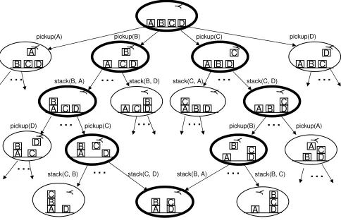
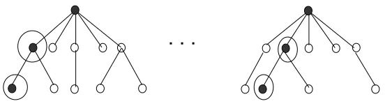
Figure 1, shows a pictorial example of a single training example from an automated planning prob-lem. The planning domain in this example is Blocksworld where individual problems involve trans-forming an initial configuration of blocks to a goal configuration using simple actions such as pick-ing up, puttpick-ing down, and stackpick-ing the various blocks. The figure shows a search space Si where
two target paths. The label Piwould encode these target paths by a sequence Pi= (Pi,0,Pi,1, . . . ,Pi,4) where Pi,j contains the set of all highlighted target nodes at depth j. A solution weight vector, for
this training example, would be required to keep at least one of the highlighted paths in the beam until uncovering the goal node.
w…
w…
…
… w…
w… w… w… pickup(B) pickup(C) stack(B, A) pickup(C)
A B C D
A
B C D A
B
C D A B
C
D A B C
D
pickup(A) pickup(D)
A B
C D A C DB A BC D A B CD
stack(B, D) stack(C, A) stack(C, D)
A B C D A B C D A B C D pickup(B)
… stack(C, D) stack(B, A) … A B C D pickup(D) A B CD
pickup(A) w… w… A B C D stack(C, B) A B C D stack(B, C)
Figure 1: An example from automated planning.
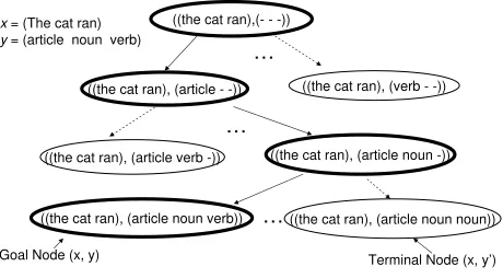
2.2.2 EXAMPLE FROMSTRUCTUREDCLASSIFICATION
((the cat ran),(- - -))
((the cat ran), (verb - -)) ((the cat ran), (article - -))
((the cat ran), (article verb -)) ((the cat ran), (article noun -))
((the cat ran), (article noun verb)) ((the cat ran), (article noun noun))
… …
…
Goal Node (x, y) x= (The cat ran) y= (article noun verb)
Terminal Node (x, y’)
Figure 2: An example from structured classification.
Thus, all of the results in this paper apply equally well to the structured-classification formulation of Daum´e III and Marcu (2005).
3. Computational Complexity
In this section, we study the computational complexity of the above consistency problems. We first focus on breadth-first beam search, and then give the corresponding best-first results at the end of this section. It is important to note that the size of the search spaces will typically be exponential in the encoding size of the learning problem. For example, in automated planning, standard languages such as PDDL (McDermott, 1998) are used to compactly encode planning problems that are po-tentially exponentially large, in terms of the number of states, with respect to the PDDL encoding size. Throughout this section we measure complexity in terms of the problem encoding size, not the potentially exponentially larger search space size. All discussions in this section apply to general search spaces and are not tied to a particular language for describing search space such as PDDL.
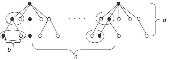
Our complexity analysis will consider various sub-classes of the breadth-first consistency prob-lem, where the sub-classes will be defined by placing constraints on the following problem param-eters: n - the number of training instances, d - the depth of target solution paths, c - the maximum number of children of any search node, t - the maximum target width of any Pias defined in Section
2.2, and b - the beam width. Figure 3 gives a pictorial depiction of these key problem parame-ters. Throughout the complexity analysis we will restrict our attention to problem classes where the maximum number of children c and beam width b are polynomial in the problem size, which are necessary conditions to ensure that each beam search step requires only polynomial time and space. We will also assume that all feature functions can be evaluated in polynomial time in the problem size.
has increased. This form of re-encoding from a search space with exponentially many children to one with polynomially many children can be done whenever the actions in the original space have a compact, factored encoding, which is typically the case in practice.
. . . .
wb
wn
d
Figure 3: The key problem parameters: n - the number of training instances, d - the depth of target solution paths, b - the beam width. Not depicted in the figure are: c - maximum number of children of any node, t - the maximum target width of any example.
3.1 Hardness Upper Bounds
We first show an upper bound on the complexity of breadth-first consistency by proving that the general problem is in NP even for exponentially large search spaces.
Observe that given a weight vector w and beam width b, we can easily generate a unique depth
d beam trajectory for each training instance. Our upper bound is based on considering the inverse
problem of checking whether a set of hypothesized beam trajectories, one for each training instance, could have been generated by some weight vector. The algorithm TestTrajectories in Figure 4 efficiently carries out this check. The main idea is to observe that for any search space S it is possible to efficiently check whether there is a weight vector that starting with a beam B could generate a beam B′after one step of breadth-first beam search. This can be done by constructing an appropriate set of linear constraints on the weight vector w that are required to generate B′ from B. In particular, we first generate the set of candidate nodes C from B by unioning all children of nodes in B. Clearly we must have B′⊆C in order for there to be a solution weight vector. If this is the
case then we create a linear constraint for each pair of nodes(u,v)such that u∈B′and v∈C−B′, which forces u to be preferred to v:
w·f(u)>w·f(v)
where w= (w1,w2, . . . ,wm) are the constraint variables and f(·) = (f1(·),f2(·), . . . ,fm(·)) is the vector of feature functions. Note that if u is more preferred than v in the total preference ordering, then we only need to require that w·f(u)≥w·f(v). The overall algorithmTestTrajectories simply creates this set of constraints for each consecutive pair of beams in each beam trajectory and then tests to see whether there is a w that satisfies all of the constraints.
Proof It is straightforward to show that w satisfies the constraints generated byTestTrajectories iff for each i,j, r(v′,v|<i,w) leads beam search to generate Bi,j+1 from Bi,j. The linear program
contains m variables and at most ndcb2 constraints. Since we are assuming that the maximum number of children of a node v is polynomial in the size of the learning problem, the size of the linear program is also polynomial and thus can be solved in polynomial time (Khachiyan, 1979). This lemma shows that sets of beam trajectories can be used as efficiently-checkable certificates for breadth-first consistency, which leads to an upper bound on the problem’s complexity.
Theorem 4 Breadth-first consistency is in NP.
Proof Given a learning problemh{hSi,Pii},bi our certificates correspond to sets of beam
trajec-tories{(Bi,0, . . . ,Bi,d)}each of size at most O(ndb)which is polynomial in the problem size. The
certificate can then be checked in polynomial time to see if for each i, (Bi,0, . . . ,Bi,d) contains a
target solution path encoded in Pi as required by Definition 1. If it is consistent then according to
Lemma 3 we can efficiently decide whether there is a w that can generate{(Bi,0, . . . ,Bi,d)}.
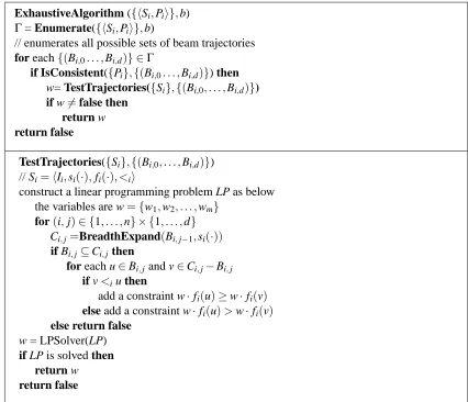
This result suggests an enumeration-based decision procedure for breadth-first consistency as given in Figure 4. In that procedure, the function Enumerate creates a list of all possible combi-nations of beam trajectories for the training data. Thus, each element of this list is a list of beam trajectories, one for each training example, where a beam trajectory is simply a sequence of sets of nodes that are selected from the given search space. For each enumerated combination of beam tra-jectories, the function IsConsistent checks whether the beam trajectory for each example contains a target path for that example and if soTestTrajectories will be called to determine whether there exists a weight vector that could produce those trajectories. The following gives us the worst case complexity of this algorithm in terms of the key problem parameters.
Theorem 5 The procedure ExhaustiveAlgorithm (Figure 4) decides breadth-first consistency and
returns a solution weight vector if there is a solution in time O (t+poly(m)) (cb)bdn .
Proof We first bound the number of certificates. Breadth-first beam search expands nodes in the
current beam, resulting in at most cb nodes, from which b nodes are selected for the next beam. Enu-merating these possible choices over d levels and n trajectories, one for each training instance, we can bound the number of certificates by O (cb)bdn
. For each certificate the enumeration process checks consistency with the target paths{Pi}in time O(tbdn)and then callsTestTrajectories which
runs in time poly(m,ndcb2). The total time complexity then is O tbdn+poly(m,ndcb2)
(cb)bdn
=O (t+poly(m)) (cb)bdn .
ExhaustiveAlgorithm ({hSi,Pii},b) Γ= Enumerate({hSi,Pii},b)
// enumerates all possible sets of beam trajectories
for each{(Bi,0. . . ,Bi,d)} ∈Γ
if IsConsistent({Pi},{(Bi,0. . . ,Bi,d)}) then
w= TestTrajectories({Si},{(Bi,0, . . . ,Bi,d)}) if w6=false then
return w return false
TestTrajectories({Si},{(Bi,0, . . . ,Bi,d)})
// Si=hIi,si(·),fi(·), <ii
construct a linear programming problem LP as below the variables are w={w1,w2, . . . ,wm}
for(i,j)∈ {1, . . . ,n} × {1, . . . ,d} Ci,j=BreadthExpand(Bi,j−1,si(·))
if Bi,j⊆Ci,jthen
for each u∈Bi,jand v∈Ci,j−Bi,j
if v<iu then
add a constraint w·fi(u)≥w·fi(v)
else add a constraint w·fi(u)>w·fi(v)
else return false
w = LPSolver(LP)
if LP is solved then return w return false
Figure 4: The exhaustive algorithm for breadth-first consistency.
Theorem 6 The class of breadth-first consistency problems where b=1 and t =1 is solvable in
polynomial time.
Proof Given a learning problemh{hSi,Pii},bi where Pi = (Pi,0, . . . ,Pi,d), t=1 implies that each Pi,j contains exactly one node. Since the beam width b=1, then the only way that a beam
trajec-tory(Bi,0, . . . ,Bi,d)can satisfy the condition Bi,j∩Pi,j6= /0for any i,j, is for Bi,j=Pi,j. Thus there
. . .
Figure 5: A tractable class of breadth-first consistency, where b=1 and t=1.
3.2 Hardness Lower Bounds
Unfortunately, outside of the above problem classes it appears that breadth-first consistency is com-putationally hard even under strict restrictions. In particular, the following three results show that if any one of b, d, or n are not bounded then the consistency problem is hard even when the other problem parameters are small constants.
First, we show that the problem class where n=d=t=1 but b≥1 is NP-complete. That is, a single training instance involving a depth one search space is sufficient for hardness. This problem class, resembles more traditional ranking problems and has a nice analogy in the application domain of web-page ranking, where the depth 1 leaves of our search space correspond to possibly relevant web-pages for a particular query. One of those pages is marked as a target page, for example, the page that a user eventually went to. The learning problem is then to find a weight vector that will cause for the target page to be ranked among the top b pages. Our result shows that this problem is NP-complete and hence will be exponential in b unless P=NP.
Theorem 7 The class of breadth-first consistency problems where n=1, d=1, t=1, and b≥1 is
NP-complete.
Proof Our reduction is from the Minimum Disagreement problem for linear binary classifiers,
which was proven to be NP-complete by Hoffgen et al. (1995). The input to this problem is a train-ing set T ={x+1,···,x+r1,x−1,···,x−r2}of positive and negative m-dimensional vectors and a positive integer k. A weight vector w classifies a vector as positive iff w·x≥0 and otherwise as negative. The Minimum Disagreement problem is to decide whether there exists a weight vector that commits no more than k misclassification.
Given a Minimum Disagreement problem we construct an instancehhS1,P1i,biof the breadth-first consistency problem as follows. Assume without loss of generality S1 =hI,s(·),f(·), <i. Let s(I) ={q0,q1,···,qr1+r2}. For each i∈ {1,···,r1}, define f(qi) = −x
+
i ∈Rm. For each i∈ {1,···,r2},define f(qi+r1) =x−i ∈Rm. Define f(q0) =0∈Rm, P1= ({I},{q0})and b=k+1. Define the total ordering<to be a total ordering in which qi<q0for every i=1, . . . ,r1and q0<qi
for every i=r1+1, . . . ,r1+r2.We claim that there exists a linear classifier with at most k misclas-sifications if and only if there exists a solution to the corresponding consistency problem.
First, suppose there exists a linear classifier w·x≥0 with at most k misclassifications. Using the weight vector w, we have
• for i=1,···,r1:
if w·x+i ≥0, w·f(qi) =w·(−x+i )≤0; if w·x+i <0, w·f(qi) =w·(−x+i )>0; • for i=r1+1, . . . ,r1+r2:
if w·x−i ≥0, w·f(qi) =w·x−i ≥0;
if w·x−i <0, w·f(qi) =w·x−i <0.
For i=1,···,r1+r2, the node qi in the consistency problem is ranked lower than q0 if and only if its corresponding example in the Minimum Disagreement problem is labeled correctly, is ranked higher than q0if and only if its corresponding example in the Minimum Disagreement problem is labeled incorrectly. Therefore, there are at most k nodes which are ranked higher than q0. With beam width b=k+1, the beam Bi,1is guaranteed to contain node q0, indicating that w is a solution to the consistency problem.
On the other hand, suppose there exists a solution w to the consistency problem. There are at most b−1=k nodes that are ranked higher than q0. That is, at least r1+r2−k nodes are ranked lower than q0. For i=1, . . . ,r1, qi is ranked lower than q0 if and only if w·f(qi)≤w·f(q0). For i=r1+1, . . . ,r1+r2, qi is ranked lower than q0 if and only if w·f(qi)<w·f(q0). Since
w·f(q0) =0, we have
• for i=1,···,r1:
w·f(qi)≤0⇒w·(−x+i )≤0⇒w·x+i ≥0; • for i=r1+1, . . . ,r1+r2:
w·f(qi)<0⇒w·x−i <0⇒w·xi−<0.
Therefore, using the linear classifier w·x≥0, at least r1+r2−k nodes are labeled correctly, that is, it makes at most k misclassifications.
Since the time required to construct the instancehhS1,P1i,bifrom T,k is polynomial in the size of T,k, we conclude that the consistency problem is NP-Complete even restricted to n=1, d=1 and t=1.
The next result shows that if we do not bound the number of training instances n, then the prob-lem remains hard even when the target path depth and beam width are equal to one. Interestingly, this subclass of breadth-first consistency corresponds to the multi-label learning problem as defined in Jin and Ghahramani (2002). In multi-label learning each training instance can be viewed as a bag of m-dimensional vectors, some of which are labeled as positive, which in our context correspond to the target nodes. The learning goal is to find a w that for each bag, ranks one of the positive vectors as best.
Theorem 8 The class of breadth-first consistency problems where d=1, b=1, c=6, t =3, and
n≥1 is NP-complete.
Proof The proof is by reduction from 3-SAT (Garey and Johnson, 1979), which is the following.
Let U ={u1, . . . ,um}, Q={q11∨q12∨q13, . . . ,qn1∨qn2∨qn3} be an instance of the 3-SAT
problem. Here, qi j =u or¬u for some u∈U . We construct from U,Q an instanceh{hSi,Pii},bi
of the breadth-first consistency problem as follows. For each clause qi1∨qi2∨qi3, let si(Ii) = {pi,1,···,pi,6}, Pi= ({Ii},{pi,1,pi,2,pi,3}), b=1, and the total ordering<iis defined so that pi,j<i pi,k for j=1,2,3 and k =4,5,6. Let ek ∈ {0,1}m denote a vector of zeros except a 1 in the k′th component. For each i=1, . . . ,n, j=1,2,3, if qi j =uk for some k then fi(pi,j) =ek and fi(pi,j+3) =−ek/2, otherwise if qi j =¬uk for some k then fi(pi,j) =−ek and fi(pi,j+3) =ek/2.
We claim that there exists a satisfying truth assignment if and only if there exists a solution to the corresponding consistency problem.
First, suppose that there exists a satisfying truth assignment. Let w= (w1,···,wm), where
wk =1 if uk is true, and wk =−1 if uk is false in the truth assignment. For each i=1, . . . ,n, j=1, . . . ,3, we have:
• if qi j is true, then
w·fi(pi,j) =1 and w·fi(pi,j+3) =−1/2;
• if qi j is false, then
w·fi(pi,j) =−1 and w·fi(pi,j+3) =1/2.
Note that for each clause qi1∨qi2∨qi3, at least one of the literals is true. Thus, for every set of
nodes{pi,1,pi,2,pi,3}, at least one of the nodes will have the highest rank value equal to 1, resulting in Bi,1={v}where v∈ {pi,1,pi,2,pi,3}. By the definition, the weight vector w is a solution to the consistency problem.
On the other hand, suppose that there exists a solution w = (w1, . . . ,wm) to the consistency problem. Assume the beam trajectory for each i is({Ii},{vi}). Then vi=pi,jfor some j∈ {1,2,3},
and for this i and j, qi j=ukor¬uk for some k. Let ukbe true if qi j=ukand be false if qi j=¬uk.
As long as there is no contradiction in this assignment, this is a satisfying truth assignment because at least one of{qi1,qi2,qi3}is true for every i, that is, every clause is true.
Now we will prove that there is no contradiction in this assignment, that is, any variable is assigned either true or false, but not both. Note that for any node v∈ {pi,1,pi,2,pi,3}, there always exists a node v′∈ {pi,4, . . . ,pi,6}such that:
• w·fi(v)<0⇔w·fi(v′)>0;
• w·fi(v)>0⇔w·fi(v′)<0; • w·fi(v) =0⇔w·fi(v′) =0.
Then because of the total ordering<iwe defined, the node vi=pi,jappearing in the beam trajectory,
must has w·fi(vi)>0. Assume without loss of generality that qi j=uk, then ukis assigned to be true.
Although¬uk might appear in other clauses, for example, qi′j′ =¬uk, its corresponding node pi′,j′ can never appear in the beam trajectory because w·fi′(pi′,j′) =w·(−ek) =−w·ek=−w·fi(pi,j)<0. Therefore, ukwill never be assigned false. A similar proof can be given for the case of qi j=¬uk.
Since the time required to construct the instanceh{hSi,Pii},bifrom U,Q is polynomial in the
size of U,Q, we conclude that the consistency problem is NP-Complete for the case of d=1, b=1,
Finally, we show that when the depth d is unbounded the consistency problem remains hard even when b=n=1.
Theorem 9 The class of breadth-first consistency problems where n=1, b=1, c=6, t =3, and
d≥1 is NP-complete.
Proof Assume x=h{hSi,Pii|i=1, . . . ,n},bi, where Si=hIi,si(·),fi(·), <iiand Pi= ({Ii},Pi,1), is an instance of the consistency problem with d=1, b=1, c=6 and t =3. We can construct an instance y of the consistency problem with n=1, b=1, c=6, and t=3. Let y=hhS¯1,P¯1i,biwhere
¯
S1=hI1,s¯(·),f¯(·),<¯i, and ¯P1= ({I1},P1,1,P2,1, . . . ,Pt,1). We define ¯s(·), ¯f(·),<¯ as below.
• s¯(I1) =s1(I1), ¯f(I1) = f1(I1);
• for each i=1, . . . ,n−1
∀v∈si(Ii), ¯f(v) = fi(v)and ¯s(v) =si+1(Ii+1);
∀(v,v′)∈si(Ii), ¯<(v,v′) =<i(v,v′); • ∀v∈sn(In), ¯f(v) = fn(v);
∀(v,v′)∈sn(In), ¯<(v,v′) =<n(v,v′).
Obviously, a weight vector w is a solution for the instance x if and only if w is a solution for the constructed instance y.
b n d c t Complexity
poly ≥1 ≥1 poly ≥1 NP
K K K poly ≥1 P
1 ≥1 ≥1 poly 1 P
poly 1 1 poly 1 NP-Complete
1 ≥1 1 6 3 NP-Complete
1 1 ≥1 6 3 NP-Complete
Figure 6: Complexity results for breadth-first consistency. Each row corresponds to a sub-class of the problem and indicates the computational complexity. K indicates a constant value and “poly” indicates that the quantity must be polynomially related to the problem size.
4. Convergence of Online Updates
In the previous section, we identified a limited set of tractable problem classes and saw that even very restricted classes remain NP-hard. We also saw that some of these hard classes had interesting application relevance. Thus, it is desirable to consider efficient learning mechanisms that work well in practice. Below we describe two such algorithms based on online perceptron updates.
4.1 Online Perceptron Updates
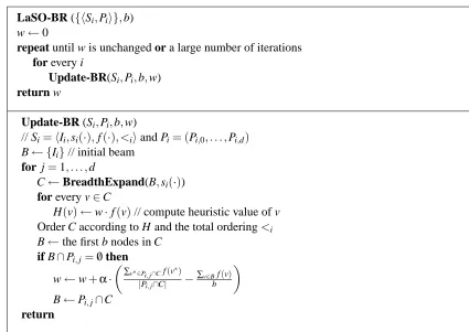
Figure 7 gives the LaSO-BR algorithm for learning ranking functions for breadth-first beam search. It resembles thelearning as search optimization (LaSO) algorithm for best-first search by Daum´e III and Marcu (2005). LaSO-BR iterates through all training instances hSi,Piiand for each one
con-ducts a beam search of the specified width. After generating the depth j beam for the ith training instance, if at least one of the target nodes in Pi,j are in the beam then no weight update occurs.
Rather, if none of the target nodes in Pi,j are in the beam then a search error is flagged and weights
are updated according to the following perceptron-style rule,
w=w+α·
∑v
∗∈Pi,j∩Cf(v∗)
|Pi,j∩C| −
∑v∈Bf(v) b
where 0<α≤1 is a learning rate parameter, B is the current beam and C is the candidate set from which B was generated (i.e., the beam expansion of the previous beam). For simplicity of notation, here we assume that f is a feature function for all training instances. Intuitively this weight update moves the weights in the direction of the average feature function of target nodes that appear in C, and away from the average feature function of non-target nodes in the beam. This has the effect of increasing the rank of target nodes in C and decreasing the rank of non-targets in the beam. Ideally, this will cause at least one of the target nodes to become preferred enough to remain on the beam next time through the search. Note that the use of averages over target and non-target nodes is important so as to account for the different sizes of these sets of nodes. After each weight update, the beam is reset to contain only the set of target nodes in C and the beam search then continues. Importantly, on each iteration, the processing of each training instance is guaranteed to terminate in
d search steps.
LaSO-BR ({hSi,Pii},b) w←0
repeat until w is unchanged or a large number of iterations for every i
Update-BR(Si,Pi,b,w)
return w
Update-BR (Si,Pi,b,w)
// Si=hIi,si(·),f(·), <iiand Pi= (Pi,0, . . . ,Pi,d) B← {Ii}// initial beam
for j=1, . . . ,d
C←BreadthExpand(B,si(·))
for every v∈C
H(v)←w·f(v)// compute heuristic value of v Order C according to H and the total ordering<i B←the first b nodes in C
if B∩Pi,j=/0then
w←w+α·
∑v∗∈Pi,j∩Cf(v∗)
|Pi,j∩C| −
∑v∈Bf(v)
b
B←Pi,j∩C
return
Figure 7: The LaSO-BR online algorithm for breadth-first beam search.
4.2 Previous Result and Counter Example
Adjusting to our terminology, Daum´e III and Marcu (2005) defined a training set to belinear separa-ble iff there is a weight vector that solves the corresponding consistency prosepara-blem. Also for linearly separable data they defined a notion of margin of a weight vector, which we refer to here as the search margin. The formal definition of search margin is given below.
Definition 10 (Search Margin) The search margin of a weight vector w for a linearly separable
training set is defined asγ=min{(v∗,v)}(w·f(v∗)−w·f(v)), where the set{(v∗,v)}contains any pair where v∗is a target node and v is a non-target node that was compared during the beam search guided by w.
LaSO-BST ({hSi,Pii},b) w←0
repeat until w is unchanged or a large number of iterations for every i
Update-BST(Si,Pi,b,w)
return w
Update-BST (Si,Pi,b,w)
// Si=hIi,si(·),f(·), <iiand Pi= (Pi,0, . . . ,Pi,d)
B← {Ii}// initial beam
¯
P=Pi,0∪Pi,2∪. . .∪Pi,d
while B∩Pi,d=/0
C←BestExpand(B,si(·))
for every v∈C
H(v)←w·f(v)// compute heuristic value of v Order C according to H and the total ordering<i B←the first b nodes in C
if B∩P¯=/0then
w←w+α·∑v∗∈P¯∩Cf(v∗)
|P¯∩C| −∑v∈B
f(v)
b
B←P¯∩C
return
Figure 8: Online algorithm for best-first beam search.
updating weights given the current beam and recomputing the beam given the updated weights. Just as traditional EM is quite prone to local minima, so are the LaSO algorithms in general, and in particular even when there is a positive search margin as demonstrated in the following counter example. Note that the standard Perceptron algorithm for classification learning does not run into this problem since there is no hidden state involved.
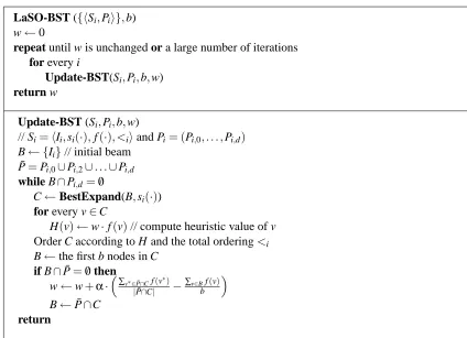
Counter Example 1 We give a training set for which the existence of a weight vector with
pos-itive search margin does not guarantee convergence to a solution weight vector for LaSO-BR or LaSO-BST. Consider a problem that consists of a single training instance with search space shown in Figure 9, preference ordering C<B<F <E <D<H <G, and single target path P= ({A},{B},{E}).
First we will consider using breadth-first beam search with a beam width of b=2. Using the
weight vector w= [γ,γ]the resulting beam trajectory will be (note that higher values of w·f(v)are better):
{A},{B,C},{E,F}.
The search margin of w, which is only sensitive to pairs of target and non-target nodes that were compared during the search, is equal to,
A
B C D
) 1 , 1 ( )
(B
f
E F G H
) 1 , 1 ( )
(E
f f(F) (0,1) f(G) (1,1) f(H) (1,1) )
1 , 0 ( )
(C
f f(D) (0,0)
) 1 , 1 ( )
(A
f
Figure 9: Counter example for convergence under positive search margin.
which is positive. We now show that the existence of w does not imply convergence under perceptron updates.
Consider simulating LaSO-BR starting from w′=0. The first search step gives the beam{D,B} according to the given preference ordering. Since B is on the target path we continue expanding to the next level where we get the new beam{G,H}. None of the nodes are on the target path so we update the weights as follows:
w′ = w′+f(E)−0.5[f(G) +f(H)] = w′+ [1,1]−[1,1]
= w′.
This shows that w′does not change and we have converged to the weight vector w′=0, which is not
a solution to the problem.
For the case of best-first beam search, the performance is similar. Given the weight vector w= [γ,γ], the resulting beam search with beam width 2 will generate the beam sequence,
{A},{B,C},{E,C}
which is consistent with the target trajectory. From this we can see that w has a positive search margin of:
γ=w·f(B)−w·f(C) =w·f(E)−w·f(C).
However, if we follow the perceptron algorithm when started with the weight vector w′=0 we can
again show that the algorithm does not converge to a solution weight vector. In particular, the first search step gives the beam{D,B}and since B is on the target path, we do not update the weights and generate a new beam{G,H}by expanding the node D. At this point there are no target nodes in the beam and the weights are updated as follows
w′ = w′+f(B)−0.5[f(G) +f(H)] = w′+ [1,1]−[1,1]
showing that the algorithm has converged to w′=0, which is not a solution to the problem.
Thus, we have shown that a positive search margin does not guarantee convergence for either LaSO-BR or LaSO-BST. This counter example also applies to the original LaSO algorithm, which is quite similar to LaSO-BST.
4.3 Convergence Under Stronger Notions of Margin
Given that linear separability, or equivalently a positive search margin, is not sufficient to guarantee convergence we consider a stronger notion of margin, thelevel margin, which measures by how much the target nodes are ranked above (or below) other non-target nodes at the same search level.
Definition 11 (Level Margin) The level margin of a weight vector w for a training set is defined as
γ=min{(v∗,v)}(w·f(v∗)−w·f(v)), where the set{(v∗,v)}contains any pair such that v∗is a target node at some depth j and v can be reached in j search steps from the initial search node—that is, v∗and v are at the same level.
For breadth-first beam search, a positive level margin for w implies a positive search margin, but not necessarily vice versa, showing that level margin is a strictly stronger notion of separability. The following result shows that a positive level margin is sufficient to guarantee convergence of LaSO-BR. Throughout we will let R be a constant such that for all training instances, for all nodes v and
v′,kf(v)−f(v′)k ≤R. The proof of this result follows similar lines as the Perceptron convergence
proof for standard classification problems Rosenblatt (1962).
Theorem 12 Given a dead-end free training set such that there exists a weight vector w with level
marginγ>0 andkwk=1, LaSO-BR will converge with a consistent weight vector after making no
more than(R/γ)2weight updates.
Proof First note that the dead-end free property of the training data can be used to show that unless
the current weight vector is a solution it will eventually trigger a “meaningful” weight update (one where the candidate set contains target nodes).
Let wkbe the weights before the k′th mistake is made. Then w1=0. Suppose the k′th mistake is made for the training datahSi,Pii, when B∩Pi,j= /0. Here, Pi,jis the j′th element of Pi, B is the
beam generated at depth j for Siand C is the candidate set from which B is selected. Note that C is
generated by expanding all nodes in the previous beam and at least one of them is in Pi,j−1. With the dead-end free property, we are guaranteed that C′=Pi,j∩C6=/0. The occurrence of the mistake
indicates that,∀v∗∈Pi,j∩C,v∈B, wk·f(v∗)≤wk·f(v), which lets us derive an upper bound for kwk+1k2.
kwk+1k2=kwk+∑v∗∈C′ f(v∗)
|C′| −
∑v∈Bf(v)
b k
2
=kwkk2+k∑v∗∈C′ f(v∗)
|C′| −
∑v∈B f(v)
b k
2
+2wk·(∑v∗∈C′ f(v∗)
|C′| −
∑v∈Bf(v)
b )
≤ kwkk2+k∑v∗∈C′ f(v∗)
|C′| −
∑v∈B f(v)
b k
2
where the first equality follows from the definition of the perceptron-update rule, the first inequality follows because wk·(f(v∗)−f(v))<0 for all v∗∈C′,v∈B, and the second inequality follows from
the definition of R. Using this upper-bound we get by induction that
kwk+1k2≤kR2.
Suppose there is a weight vector w such that||w||=1 and w has a positive level margin, then we can derive a lower bound for w·wk+1.
w·wk+1=w·wk+w·(∑v∗∈C′ f(v∗)
|C′| −
∑v∈Bf(v)
b )
=w·wk+∑v∗∈C′w·f(v∗)
|C′| −
∑v∈Bw·f(v) b
≥w·wk+γ.
This inequality follows from the definition of the level marginγof the weight vector w.
By induction, we get that w·wk+1≥kγ. Combining this result with the above upper bound on
kwk+1kand the fact thatkwk=1 we get that 1≥ w·w
k+1
kwkkwk+1k≥
√
kγ
R ⇒k≤ R2
γ2.
Without the dead-end free property, LaSO-BR might generate a candidate set that contains no target nodes, which would allow for a mistake that does not result in a weight update. However, for a dead-end free training set, it is guaranteed that the weights will be updated if and only if a mistake is made. Thus, the mistake bound is equal to the bound on the weight updates.
Note that for the example search space in Figure 9 there is no weight vector with a positive level margin since the final layer contains target and non-target nodes with identical weight vectors. Thus, the non-convergence of LaSO-BR on that example is consistent with the above result. Unlike LaSO-BR, LaSO-BST and LaSO do not have such a guarantee since their beams can contain nodes from multiple levels. This is demonstrated by the following counter example.
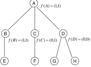
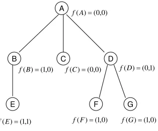
Counter Example 2 We give a training set for which the existence of a w with positive level margin
does not guarantee convergence for LaSO-BST. Consider a single training example with the search space in Figure 10, single target path P= ({A},{B},{E}), and preference ordering C<B<E<
F<G<D.
Given the weight vector w= [2γ,γ], the level margin of w is equal toγ. However, starting with w′=0 and running LaSO-BST the first search step gives the beam{D,B}. Since B is on the target path, we get the new beam{G,F}by expanding the node D. This beam does not contain a target node, which triggers the following weight update:
w′ = w′+f(B)−[f(F) +f(G)]/2
= w′+ [1,0]−[1,0]
= w′.
Since w′ does not change the algorithm has converged to w′ =0, which is not a solution to this
A
B C D
) 0 , 1 ( )
(B
f
E F G
) 1 , 1 ( )
(E
f f(F) (1,0) f(G) (1,0)
) 0 , 0 ( )
(C
f f(D) (0,1)
) 0 , 0 ( )
(A
f
Figure 10: Counter example to convergence under positive level margin.
In order to guarantee convergence of LaSO-BST, we require an even stronger notion of margin, global margin, which measures the rank difference between any target node and any non-target node, regardless of search space level.
Definition 13 (Global Margin) The global margin of a weight vector w for a training set is defined
asγ=min{(v∗,v)}(w·f(v∗)−w·f(v)), where the set{(v∗,v)}contains any pair such that v∗is any target node and v is any non-target node in the search space.
Note that if w has a positive global margin then it has a positive level margin. The converse is not necessarily true. The global margin is similar to the common definitions of margin used to characterize the convergence of linear perceptron classifiers (Novikoff, 1962).
To ensure convergence of LaSO-BST we also assume that the search spaces are all finite trees. This avoids the possibility of infinite best-first beam trajectories that never terminate at a goal node. Tree structures are quite common in practice and it is often easy to transform a finite search space into a tree. The structured classification experiments of Daum´e III and Marcu (2005) and our own automated experiments both involve tree structured spaces.
Theorem 14 Given a dead-end free training set of finite tree search spaces such that there exists a
weight vector w with global marginγ>0 andkwk=1, LaSO-BST will converge with a consistent
weight vector after making no more than(R/γ)2weight updates.
The proof is similar to that of Theorem 12 except that the derivation of the lower bound makes use of the global margin and we must verify that the restriction to finite tree search spaces guarantees that each iteration of LaSO-BST will terminate with a goal node being reached. We were unable to show convergence for the original LaSO algorithm even under the assumptions of this theorem.
to linear separability, but is not enough to guarantee convergence for either algorithm. This is in contrast to results for linear classifier learning, where linear separability implies convergence of perceptron updates.
4.4 Convergence for Ambiguous Training Data
Here we study convergence for linearly inseparable training data. Inseparability is often the result of training-data ambiguity, in the sense that many “good” solution paths are not included as tar-get paths. For example, this is common in automated planning where there can be many (nearly) optimal solutions, many of which are inherently identical (e.g., differing in the orderings of un-related actions). It is usually impractical to include all solutions in the training data, which can make it infeasible to learn a ranking function that strictly prefers the target paths over the inherently identical paths not included as targets. In these situations, the above notions of margin will all be negative. Here we consider the notion ofbeam margin that allows for some amount of ambiguity, or inseparability.
For each instancehSi,Pii, where Si=hIi,si(·),f(·), <iiand Pi = (Pi,1,Pi,2, . . . ,Pi,di), let Di j be
the set of nodes that can be reached in j search steps from Ii. That is, Di j is the set of all possible
non-target nodes that could be in beam Bi,j. A beam margin is a triple(b′,δ1,δ2) where b′ is a non-negative integer, andδ1,δ2≥0.
Definition 15 (Beam Margin) A weight vector w has beam margin (b′,δ1,δ2) on a training set
{hSi,Pii}, if for each i,j there is a set D′i j⊆Di jsuch that|D′i j| ≤b′and
∀v∗∈Pi,j,v∈Di j−D′i j, w·f(v∗)−w·f(v)≥δ1and,
∀v∗∈Pi,j,v∈D′i j, δ1>w·f(v∗)−w·f(v)≥ −δ2.
A weight vector w has beam margin(b′,δ1,δ2)if at each search depth it ranks the target nodes better than most other non-target nodes (those in Di j−D′i j) by a margin of at leastδ1, and ranks at most b′
non-target nodes (those in D′i j) better than the target nodes by a margin no greater thanδ2. Whenever this condition is satisfied we are guaranteed that a beam search of width b>b′ guided by w will solve all of the training problems. The case where b′=0 corresponds to the level margin, where the data is separable. By allowing b′>0 we can consider cases where there is no “dominating” weight vector that ranks all targets better than all non-targets at the same level. The following result shows that for a large enough beam width, which is dependent on the beam margin, LaSO-BR will converge to a consistent solution.
Theorem 16 Given a dead-end free training set, if there exists a weight vector w with beam margin
(b′,δ1,δ2)andkwk=1, then for any beam width b>(1+δ2/δ1)b′=b∗, LaSO-BR will converge
with a consistent weight vector after making no more than(R/δ1)2 1−b∗b−1 −2
weight updates.
Proof Let wk be the weights before the k′th mistake is made, so that w1=0. Suppose that the k′th mistake is made when B∩Pi,j = /0 where B is the beam generated at depth j for the ith training
instance. We can derive the upper bound ofkwk+1k2≤kR2as in the proof of Theorem 12.
w·wk+1=w·wk+w·(∑v∗∈C′ f(v∗)
|C′| −
∑v∈Bf(v)
b )
=w·wk+w·
∑
v∈B−B′
∑v∗∈C′f(v∗)
|C′| −f(v) b
+w·
∑
v∈B′
∑v∗∈C′f(v∗)
|C′| −f(v) b
≥w·wk+(b−b′)δ1
b −
b′δ2
b .
By induction, we get that w·wk+1 ≥k(b−b′)δ1−b′δ2
b . Combining this result with the above upper
bound onkwk+1kand the fact thatkwk=1 we get that 1≥ w·wk+1 kwkkwk+1k≥
√
k(b−b′)δ1−b′δ2
bR . The mistake
bound follows by noting that b>b∗and algebra.
Similar to Theorem 12, the dead-end free property of the training set guarantees that the mistake bound is equal to the bound on the weight updates.
Note that when there is a positive level margin (i.e., b′=0), the mistake bound here reduces to
(R/δ1)2, which does not depend on the beam width and matches the result for separable data. This is also the behavior when b>>b∗.
An interesting aspect of this result is that the mistake bound depends on the beam width. Rather, all of our previous convergence results were independent of the beam width and held even for beam width b=1. Thus, those previous results did not provide any formalization of the intuition that the learning problem will often become easier as the beam width increases, or equivalently as the amount of search increases. Indeed, in the extreme case of exhaustive search, no learning is needed at all, whereas for b=1 the ranking function has little room for error.
To get a sense for the dependence on the beam width consider two extreme cases. As noted above, for very large beam widths such that b>>b∗, the bound becomes(R/δ1)2. On the other extreme, if we assumeδ1=δ2and we use the smallest possible beam width allowed by the theorem
b=2b′+1, then the bound becomes((2b′+1)R/δ1)2, which is a factor of(2b′+1)2 larger than when b>>b′. This shows that as we increase b (i.e., the amount of search), the mistake bound decreases, suggesting that learning becomes easier, agreeing with intuition.
It is also possible to define an analog to the beam margin for best first beam search. However, in order to guarantee convergence, the conditions on ambiguity would be relative to the global state space, rather than local to each level of the search space.
5. Application to Automated Planning