STORE: Sparse Tensor Response Regression and
Neuroimaging Analysis
Will Wei Sun [email protected]
Department of Management Science
University of Miami School of Business Administration Miami, FL 33146, USA
Lexin Li [email protected]
Division of Biostatistics University of California Berkeley, CA 94720, USA
Editor:Animashree Anandkumar
Abstract
Motivated by applications in neuroimaging analysis, we propose a new regression model, Sparse TensOr REsponse regression (STORE), with a tensor response and a vector predic-tor. STORE embeds two key sparse structures: element-wise sparsity and low-rankness. It can handle both a non-symmetric and a symmetric tensor response, and thus is applicable to both structural and functional neuroimaging data. We formulate the parameter estima-tion as a non-convex optimizaestima-tion problem, and develop an efficient alternating updating algorithm. We establish a non-asymptotic estimation error bound for the actual estimator obtained from the proposed algorithm. This error bound reveals an interesting interaction between the computational efficiency and the statistical rate of convergence. When the distribution of the error tensor is Gaussian, we further obtain a fast estimation error rate which allows the tensor dimension to grow exponentially with the sample size. We illus-trate the efficacy of our model through intensive simulations and an analysis of the Autism spectrum disorder neuroimaging data.
Keywords: Functional connectivity analysis, High-dimensional statistical learning, Mag-netic resonance imaging, Non-asymptotic error bound, Tensor decomposition
1. Introduction
In this article, we study a class of high-dimensional regression models with a tensor response and a vector predictor. Tensor, a.k.a. multidimensional array, is now frequently arising in a wide range of scientific and business applications (Yuan and Zhang, 2016). Our moti-vation comes from neuroimaging analysis. One example is anatomical magnetic resonance imaging (MRI), where the data takes the form of a three-dimensional array, and image voxels correspond to brain spatial locations. Another example is functional magnetic reso-nance imaging (fMRI), where the goal is to understand brain functional connectivity that is encoded by a symmetric matrix, with rows and columns corresponding to brain regions, and entries corresponding to interaction between those regions. In both examples, it is of keen scientific interest to compare the scans of brains, or the brain connectivity patterns, between the subjects with neurological disorder and the healthy controls, after adjusting
c
for additional covariates such as age and sex. Both can be more generally formulated as a regression problem, with image tensor or connectivity matrix serving as a response, and the group indicator and other covariates forming a predictor vector.
1.1 Our Proposal
We develop a general class of tensor response regression models, namely STORE, and embed two key sparse structures: element-wise sparsity and low-rankness. Both structures serve to greatly reduce the computational complexity of the estimation procedure. Meanwhile, both are scientifically plausible in plenty of applications, and have been widely employed in high-dimensional multivariate regressions (e.g., Tibshirani, 1996; Zou, 2006; Yuan and Lin, 2006; Peng et al., 2010; Zhou et al., 2013; Raskutti and Yuan, 2016). A unique feature of STORE is that, it can not only handle a non-symmetric tensor response, but also a symmetric tensor response, and thus is applicable to both structural and functional neuroimaging analysis.
We formulate the learning of STORE as a non-convex optimization problem, and ac-cordingly develop an efficient alternating updating algorithm. Our algorithm consists of two major steps, and each step iteratively updates a subset of the unknown parameters while fixing the others. In Step 1, we reformulate the estimation as a sparse tensor decomposition problem and then employ a decomposition algorithm, the truncated tensor power method (Sun et al., 2017), for solution. In Step 2, we utilize the bi-convex structure of the problem to obtain a closed-form solution.
We carry out a non-asymptotic theoretical analysis for the actual estimator obtained from our optimization algorithm. Based upon a set of our newly developed techniques to tackle the non-convexity in estimation, we obtain an explicit error bound of the actual minimizer. Specifically, let Ei, i= 1, . . . , n, denote the error tensor, and Θ∗ denote the set of all true parameters. Given an initial parameter with an initialization error , the finite sample error bound of thet-th step solution Θb(t) consists of two parts:
D
b Θ(t),Θ∗
≤ κt |{z} computational error
+ 1
1−κmax (
C·η 1 n
n
X
i=1 Ei, s
! ,√Ce
n )
| {z }
statistical error
,
with a high probability. Hereκ∈(0,1) is a contraction coefficient,C andCeare some
posi-tive constants, andη n−1Pn
i=1Ei, s
represents the s-sparse spectral norm of the averaged error tensor; see (8) for a formal definition of this norm. This error bound portrays the estimation error in each iteration, and reveals an interesting interplay between the compu-tational efficiency and the statistical rate of convergence. Note that the compucompu-tational error decays geometrically with the iteration number t, whereas the statistical error remains the same whentgrows. Therefore, this bound provides a meaningful guidance for the maximal number of iterationsT. That is, we stop when the computational error becomes dominated by the statistical error. The resulting estimator falls within the statistical precision of the true parameterΘ∗. Additionally, this finite sample error bound provides a general theoret-ical guarantee of our estimator, and the result holds for any distribution of the error tensor Ei, by noting that it relies onEionly through its sparse spectral normη n−1Pni=1Ei, s
Eiis available. In particular, when the third-order error tensorEi ∈Rd1×d2×d3,i= 1,· · ·, n,
follows an i.i.d. Gaussian distribution, we have
DΘb(T),Θ∗
=Op
r
s3log(d 1d2d3) n
! ,
where s is the cardinality parameter of the decomposed components in the tensor coeffi-cients. This fast estimation error rate allows the tensor dimension to grow exponentially with the sample size. When the order of the tensor is one, STORE reduces to the d -dimensional vector regression and our statistical error reduces toOp(
p
slogd/n), which is known to be minimax optimal (Wang et al., 2014).
1.2 Related Works and Our Contributions
Our work is related to but also clearly distinct from a number of recent development in high-dimensional statistical models involving tensor data.
The first is a class of tensor decomposition methods (Chi and Kolda, 2012; Liu et al., 2012; Anandkumar et al., 2014a,b; Yuan and Zhang, 2016; Sun et al., 2017). Tensor decom-position is an unsupervised learning method that aims to find the best low-rank approxi-mation of a single tensor. Our proposed tensor response regression, however, is asupervised
learning method, which aims to estimate the coefficient tensor that characterizes the as-sociation between the tensor response and the vector predictor. Although we utilize the sparse tensor decomposition step of Sun et al. (2017) as part of our estimation algorithm, our objective and technical tools involved are completely different. Particularly, because we work withmultiple tensor samples, the consistency of our estimator is indexed by both the tensor dimension and the sample size. This is different from the sparse tensor decomposition estimator in Sun et al. (2017) that works with asingle tensor only. Consequently, new large deviation inequalities are needed and derived in our theoretical investigation. Moreover our algorithm is not restricted to any particular decomposition procedure but can be coupled with other decomposition solutions, e.g., Chi and Kolda (2012); Liu et al. (2012).
The second related line of research tackles tensor regression where the response is a scalar and the predictor is a tensor (Zhou et al., 2013; Wang and Zhu, 2017; Yu and Liu, 2016). In those papers, a low-rank structure is often imposed on the coefficient tensor, which is similar to the low-rank principle we also employ. However, they all treated the tensor as apredictor, whereas we treat it as aresponse. This difference in modeling approach leads to different focus and interpretation. The tensor predictor regression focuses on understanding the change of a biological outcome as the tensor image varies, while the tensor response regression aims to study the change of the image as the predictors such as the disease status and age vary. When it comes to theoretical analysis, the two models involve utterly different techniques. In a way, their difference is in analogous to that between multi-response regression and multi-predictor regression in the classical vector-valued regression context.
In particular, Zhu et al. (2009) considered a 3×3 symmetric positive definite matrix arising from diffusion tensor imaging as a response, and developed an intrinsic regression model by mapping the Euclidean space of covariates to the Riemannian manifold of positive-definite matrices. Unlike their solution, we consider a non-symmetric or symmetric tensor response in the Euclidean space, and allow the dimension of the tensor response to increase with the sample size. Li et al. (2011) estimated regression parameters by building iteratively increasing neighbors around each voxel and smoothing observations within the neighbors with weights. By contrast, we model all the voxels in an image tensor in a joint fashion.
Rabusseau and Kadri (2016) considered a tensor response model with a low-rank struc-ture. However, no sparsity is enforced in their estimator, and thus their method is not directly applicable for selecting brain subregions affected by the disorder. Our approach instead is capable of region selection, and the resulting estimator is much easier to interpret. Li and Zhang (2017) proposed an envelope-based tensor response model that is notably different from our proposal. First, they utilized a generalized sparsity principle to exploit the redundant information in the tensor response, by seeking linear combinations of the response that are irrelevant to the regression. Our method instead utilizes the element-wise sparsity in terms of the individual entries. As such our method can achieve region selection, whereas their approach cannot. Second, they obtained the √n-convergence rate for the
global minimizer of their objective function when the tensor dimension is fixed. However, their objective function is non-convex and there is no guarantee that the optimization algorithm can find this global minimizer. By contrast, we derive the error rate of the
actual minimizer of our algorithm at each iteration, and we also permit an increasing tensor dimension. Third, their approach could not directly incorporate the symmetry constraint when the tensor response is symmetric, which is often encountered in functional imaging analysis. To the best of our knowledge, our solution is the first that can simultaneously tackle both a non-symmetric and a symmetric tensor response in a regression setup.
Raskutti and Yuan (2016) developed a class of sparse regression models, under the assumption of Gaussian error, when either or both the response and predictor are tensors. When the error distribution is Gaussian, our error bound matches theirs. However, our bound is obtained for a general error distribution, where the normality is not necessarily required. In addition, they required another crucial condition that the regularizer must be convex and weakly decomposable. We do not impose this assumption, but instead tackle a non-convex optimization problem, and employ a different set of proof techniques. Finally, they achieved the low-rankness of the estimator through a tensor nuclear norm, which is known to be computationally NP-hard (Friedland and Lim, 2014). By contrast, our rate is established for the actual estimator obtained from our optimization algorithm, which we show later is both feasible and scalable.
establish the convergence for the population and sample optimizers then combine the two. By contrast, our analysis hinges on exploitation of the bi-convex structure of the objective function, as well as a careful characterization of the impact of the intermediate sparse tensor decomposition step on the estimation error in each iteration step. The bi-convex structure frequently arises in many optimization problems. As such tools we develop are also of independent interest, and enrich the current toolbox of non-convex optimization analysis.
1.3 Notations and Structure
Throughout the article we adopt the following notations. Denote [d] = {1, . . . , d}, and Id the d×d identity matrix. Denote 1(·) the indicator function, and ◦ the outer product between vectors. For a vector a = Rd, kak denotes its Euclidean norm, and kak0 the L0
norm, i.e., the number of nonzero entries in a. For a matrix A ∈ Rd×d, kAk denotes its spectral norm. For a tensor A ∈ Rd1×...×dm, and a set of vectors a
j ∈ Rdj, j = 1, . . . , m,
the multilinear combination of the tensor entries is defined as A ×1 a1 ×2. . .×mam :=
P
i1∈[d1]. . .
P
im∈[dm]ai1. . . aimAi1,...,im ∈R. The tensor spectral norm is defined as kAk:= supka1k=...=kamk=1|A ×1 a1 ×2 . . .×m am|, and the tensor Frobenius norm as kAkF := q
P
i1,...,imA 2
i1,...,im. For two tensors A,B ∈ R
d1×...×dm, their inner product is hA,Bi =
P
i1,...,imAi1,...,imBi1,...,im. See Kolda and Bader (2009) for more tensor operations. We say an=o(bn) if an/bn converges to 0 asnincreases to infinity.
The rest of the article is organized as follows. Section 2 introduces the proposed sparse tensor response regression model, and Section 3 presents the optimization algorithm. Sec-tion 4 establishes the estimaSec-tion error bound. SecSec-tion 5 presents the simulaSec-tion results, and Section 6 applies our method to an analysis of the Autism spectrum disorder imaging data. The appendix collects all technical proofs.
2. Model
For an mth-order tensor response Yi ∈ Rd1×···×dm, and a vector of predictors xi ∈ Rp, i= 1, . . . , n, we consider the tensor response regression model of the form,
Yi =B∗×m+1xi+Ei, (1) whereB∗ ∈
Rd1×···×dm×p is an (m+ 1)th-order tensor coefficient, andEi ∈Rd1×···×dm is an
error tensor independent of xi. Without loss of generality, the intercept is set to zero, by centering the samples xi and Yi. We also usedm+1 := p to represent the dimension ofxi. Our goal is to estimateB∗ given ni.i.d. observations {(x
i,Yi), i= 1, . . . , n}.
To facilitate estimation of the ultrahigh dimensional unknown parameters under a lim-ited sample size, it is crucial to introduce some sparse structures. Two most commonly used structures are element-wise sparsity and low-rankness (Raskutti and Yuan, 2016). In the context of tensor response regression, we assume thatB∗ admits the following rank-K
decomposition structure (Kolda and Bader, 2009),
B∗ = X k∈[K]
where Sd={v∈Rd| kvk= 1},kβk,j∗ k0 ≤dj0 < dj, and dj0 represents the true sparsity of
the individual componentsβ∗k,j, fork∈[K],j∈[m+ 1]. Consequently, when coupling with the low-rank structure of (2), the element-wise sparsity ofβk,j∗ implies that some individual entries of B∗ are zero. Moreover, we assume w∗
max = w1∗ ≥ · · · ≥ wK∗ = w∗min > 0, and
assume eachwi∗ to be bounded away from 0 and∞. Under the structure of (2), estimating B∗ reduces to the estimation ofwk∗, βk,∗1, . . . , β∗k,m+1 for any k∈[K], and the corresponding parameter space becomes B := {wk ∈ R,βk,j ∈ Rdj, k ∈ [K], j ∈ [m+ 1]|c1 ≤ |wk| ≤
c2,kβk,jk2= 1,kβk,jk0 ≤dj0}.Accordingly, the number of unknown parameters is reduced
from pQm
j=1dj toK( Pm
j=1dj+p). To estimate those unknown parameters, we propose to
solve the following constrained optimization problem,
min wk,βk,1,...,βk,m+1
k∈[K],j∈[m+1]
1
n
n
X
i=1 Yi−
X
k∈[K]
wk(βk,m> +1xi)βk,1◦ · · · ◦βk,m
2
F, (3)
subject tokβk,jk2= 1,kβk,jk0 ≤sj,
wheresjis the cardinality parameter of thej-th component. Here we encourage the sparsity of the decomposed components via a hard-thresholding penalty to control kβk,jk0.
Com-pared to the lasso type penalized approach in sparse learning, the hard-thresholding method avoids bias and has been shown to be more appealing in numerous high-dimensional learning problems (Shen et al., 2012, 2013; Wang et al., 2014).
3. Estimation
The problem in (3) is a non-convex optimization. The key of our estimation procedure is to explore its bi-convex structure. In particular, the objective function in (3) is bi-convex in (βk,1, . . . ,βk,m+1),k∈[K], in that it is convex in βk,j when all other parameters are fixed. Utilizing this property, we propose an efficient alternating updating algorithm to solve (3).
3.1 Algorithm
We first summarize our estimation procedure in Algorithm 1, then present the two key alternative steps.
Step 1: The first core step of our algorithm is to update wk,βk,1, . . . ,βk,m for each
k = 1, . . . , K, given βj,m+1, j = 1, . . . , K and wk0, βk0,1, . . . , βk0,m, k0 6=k. Letting αik :=
β>k,m+1xi,i= 1, . . . , n, we note that (3) is equivalent to
min wk,βk,1,...,βk,m
kβk,jk2=1,kβk,jk0≤sj,j∈[m]
1
n
n
X
i=1 α2ik
Ri−wkβk,1◦ · · · ◦βk,m 2
F, (4)
where the residual tensor term Ri is of the form,
Ri :=hYi− X
k06=k,k0∈[K]
wk0αik0βk0,1◦ · · · ◦βk0,m
i
/αik. (5)
Algorithm 1 Alternating updating algorithm for STORE.
1: Input: data{(xi,Yi), i= 1, . . . , n}, rank K, cardinality vector (s1, . . . , sm).
2: Initializewk= 1 and random unit-norm vectors βk,1, . . . ,βk,m+1 for each k∈[K]. 3: Untilthe termination condition is met, Do
4: Step 1: Fork= 1 toK, obtainwbk,βbk,1, . . . ,βbk,mby solving (6) via the sparse tensor
decomposition procedure of Sun et al. (2017) with parameters K and (s1, . . . , sm).
5: Step 2: For k= 1 to K, obtain βbk,m+1 using Lemma 2. 6: Output: wbk,βbk,1, . . . ,βbk,m+1 for each k∈[K].
Lemma 1 Denote(wbk,βbk,1, . . . ,βbk,m)as the solution of(4), and denote( e
wk,βek,1, . . . ,βek,m) as the solution of
min wk,βk,1,...,βk,m
kβk,jk2=1,kβk,jk0≤sj,j∈[m]
¯
R −wkβk,1◦ · · · ◦βk,m
2
F, (6)
where R¯ := n1 Pn
i=1αik2Ri. Then it satisfies that wbk =nwek/ Pn
i=1α2ik and βbk,l =βek,l, for l= 1, . . . , m and k= 1, . . . , K.
Lemma 1 implies that the optimization problem in (4) reduces to a sparse rank-one tensor decomposition on the averaged tensor ¯R. To efficiently solve (6), in this paper we employ a truncation-based sparse tensor decomposition procedure (Sun et al., 2017), by first solving the non-sparse tensor decomposition components and then truncating them to achieve the desirable sparsity. It is also noteworthy that our method is flexible in the choice of opti-mization algorithm for solving (6), and Algorithm 1 can be coupled with many other sparse tensor decomposition algorithms, e.g., Chi and Kolda (2012); Liu et al. (2012).
When the tensor responseYiis symmetric, the resulting coefficientBshould be symmet-ric too. Our algorithm can easily adapt to this scenario, by settingβk,1=· · ·=βk,m=βk for each k ∈ [K], and the cardinality parameters s1 = · · ·= sm = s. That is, we slightly modify Step 1 in Algorithm 1 as: for k= 1 toK, compute Ri in (5) and solve wbk,βbk via
the symmetric sparse tensor decomposition with parametersK and s.
Step 2: The second core step of our algorithm is to updateβk,m+1for eachk= 1, . . . , K,
given wj, βj,1, . . . ,βj,m,j= 1, . . . , K and βk0,m+1,k0 6=k. LettingAk=wkβk,1◦ · · · ◦βk,m,
then (3) is equivalent to
min α
1
n
n
X
i=1 Ti−α
>x
iAk
2
F, (7)
where the residual tensor Ti=Yi−Pk06=k,k0∈[K]wk0(β>
k0,m+1xi)βk0,1◦ · · · ◦βk0,m. The next
lemma gives a closed-form solution of (7).
Lemma 2 The solution of (7) is given by
b
βk,m+1 =
1
n
n
X
i=1 xix>i
!−1
n−1Pn
i=1hTi,Akixi kAkk2F
In our neuroimaging example in Section 6, the dimension of the predictor vector is
p= 3. For such a small value of p, the sample size nis generally much larger, and we can directly invert the sample covariance matrix n−1Pn
i=1xix>i . If n < p, this matrix is not invertible. Then one may employ sparse graphical model estimation (Yuan and Lin, 2007; Friedman et al., 2008; Zhang and Zou, 2014) and replace this inverse with a sparse precision matrix estimator. Alternatively, one may also introduce additional sparsity constraint on the parameterβk,m+1 and resort to a regularized estimation approach to update βk,m+1.
Finally, we terminate the alternating update of Steps 1 and 2 when the new estimates are close to the ones from the previous iteration. The termination condition is set as
max
j∈[m+1],k∈[K]min n
kβb (t)
k,j−βb (t−1)
k,j k,kβb (t)
k,j+βb (t−1)
k,j k
o
≤10−4.
3.2 Tuning Parameter Selection
In Algorithm 1, the rank K and the cardinality s1, . . . , sm are tuning parameters. We propose to select those parameters via a BIC-type criterion. Specifically, given a pre-specified set of rank values K and a pre-specified set of cardinality values S1, . . . ,Sm, we choose the combination of parameters (K,b sb1, . . . ,sbm) that minimizes
BIC = log n
X
i=1
kYi−B ×b m+1xik2F !
+log(n
Qm j=1dm)
nQm
j=1dm
K
X
k=1
m
X
j=1
kβbk,jk0.
This criterion balances between model fitting and model sparsity, and a similar version has been commonly employed in rank estimation (Zhou et al., 2013).
4. Theory
Next we establish the error bound of the actual STORE estimator obtained from our Algo-rithm 1. The resulting error bound consists of two quantities: a computational error and a statistical error. The computational error captures the error caused by the non-convexity of the optimization, whereas the statistical error measures the error due to finite samples.
In order to compute the distance between the estimator and the truth, we define the distance measure between two unit vectors u,v ∈ Rd as D(u,v) := p
1−(u>v)2. We
then have D(u,v)≤min{ku−vk,ku+vk} ≤√2D(u,v). The distance functionD(u,v) resolves the sign issue in the decomposition components since changing the signs of any two component vectors does not affect the generated tensor.
4.1 Assumptions
We first introduce the technical assumptions required to guarantee the desirable error bound. The first assumption is about the structure of the true model.
Assumption 3 (Model Assumption) In model(1), we assume the true coefficientB∗ is sparse and low-rank satisfying (2) and such decomposition is unique up to a permutation. Assume kB∗k ≤ C1wmax∗ , and for each i, assume kxik ≤ C2 and |β∗>k,m+1xi| ≥ C3 almost
the sample covariance Σ := n−1Pn
i=1xix>i to satisfy c0 < λmin(Σ) ≤ λmax(Σ) < ce0 for some constants c0,c0.e
The above unique decomposition condition is to ensure the identifiability of tensor decom-position. Kruskal (1976, 1977) provided the classical conditions for such identifiability if the sum of the Kruskal ranks of them decomposed component matrices is larger than 2K+ 2. In our model, the rankK is fixed, and hence the identifiability of our tensor decomposition (2) is guaranteed when the decomposed components are not highly dependent. Moreover, the conditions on the predictor vector xi are mild and trivially hold when the dimension of
xi is fixed. In Section 6, the dimension of xi is 3 in our neuroimaging data example. The second assumption is about the initialization in Algorithm 1.
Assumption 4 (Initialization Assumption) Define the initialization error
:= max
max k kwb
(0)
k −w
∗
kk2,max k,j D
b
β(0)k,j,βk,j∗
.
We assume that
<min
(s
wmin∗
2(w∗min+w∗
maxC1)
, w
∗2
min
8√5w∗maxC1(6√2w∗min+ 2),
C3
2C2, w∗min
2
) ,
where the constants C1, C2, C3 are as defined in Assumption 3.
Note that our assumption on the initialization parameters only requires the error to be bounded by some constant; i.e., the initial estimators are not too far away from the true parameters. This assumption is necessary to handle the non-convexity of the optimization, and has been commonly imposed in non-convex optimization (Wang et al., 2014; Balakrish-nan et al., 2017). It is also noteworthy that this assumption is satisfied by the estimators from sparse singular value decomposition of the unfolding matrix from the original tensor in Step 1 of Algorithm 1; see Sun et al. (2017) for more discussion on the theoretical guarantee of such an initialization procedure.
The third assumption requires that the error tensor Ei is controlled. Before stating the assumption, we introduce a critical concept to measure the noise level in the tensor response regression. In particular, we define the sparse spectral norm ofE as
η(E, d01,· · ·, d0m) := sup
ku1k=···=kumk=1
ku1k0≤d01,...,kumk0≤d0m
E ×1u1×2· · · ×mum
. (8)
This quantifies the perturbation error in a sparse scenario, and in the sparse case with
d0j dj (j= 1, . . . , m), it is much smaller than the spectral normkEk, i.e.,η(E, d1,· · ·, dm). Denotingd0= maxjd0j, we haveη(E, d01,· · · , d0m)≤η(E, d0,· · · , d0). We writeη(E, d0) := η(E, d0,· · · , d0).
Assumption 5 (Error Assumption) Let s:= max{s1, . . . , sm}, with sj being the
cardi-nality parameter in Algorithm 1. We assume the error tensorEi, i= 1, . . . , n, satisfies
η 1 n
n
X
i=1 Ei, s
!
≤ C3w
∗
min
8 ,
This assumption requires that the observed tensor responses, Yi,i= 1, . . . , n, are not too noisy. It is a minor condition, since we only require the spectral norm of the error tensor to be bounded. As we later show in Section 4.3, whenEi is a standard Gaussian tensor, its spectral norm converges to zero when the sample size nincreases.
4.2 Main Result
Next we present our main theorem that describes the estimation error of the actual estimator at each iteration from Algorithm 1.
Theorem 6 Assuming Assumptions 3, 4, and 5, the estimator in the t-th iteration of Algorithm 1, with s≥d0:= maxjdj0, satisfies that
max
max k kwb
(t)
k −w
∗
kk2,max
k,j D
b
β(k,jt),β∗k,j
≤ κt
|{z}
computational error
+ 1
1−κmax (
4√5
C3w∗minη
1
n
n
X
i=1 Ei, s
! ,√Ce
n )
| {z }
statistical error
, (9)
where the contraction coefficient κ = (κ1+κ2)κ3 ∈ (0,1), with κ1 := 4√5wmax∗ C3/wmin∗ , κ2 := 2C2η E¯, s
/C32, and κ3 := 2/w∗min+ 6 √
2. Here C1, C2, C3 are constants as defined in Assumption 3, and Ce is some positive constant.
Theorem 6 reveals the interplay between the computational error and the statistical error for our estimator, and has some interesting implications. First, it provides a theoretical guidance to terminate the iterations of the alternating updating algorithm. That is, when the computational error is dominated by the statistical error, in that
t≥T := log1/κ
(1−κ)
max
n 4√5
C3w∗minη
1
n
Pn
i=1Ei, s
,√Ce
n
o
, (10)
the estimator from our algorithm achieves an error at the rate
Op max
( η 1
n
n
X
i=1 Ei, s
! ,√1
n )!
. (11)
The constantsC3andCein (10) are unknown in practice. However, due to the fact both
con-stants are independent of the sample size, the sparsity parameters, and the dimensionality, the expression (10) gives an order of the optimal terminationT in terms of the parameters that go to infinity. Second, Theorem 6 also provides a general theoretical guarantee for our estimator for any distribution of the error tensor Ei, as the error rate depends on the distribution of the error tensor only through η 1nPn
i=1Ei, s
. Later we obtain the explicit forms of the error rates for some special error distributions.
4.3 Gaussian Tensor Error
We derive the explicit form of the statistical error in Theorem 6 when Ei, i= 1, . . . , n, are i.i.d. Gaussian tensors; i.e., the entries of Ei are i.i.d. standard Gaussian random variables.
Corollary 7 Under the assumptions of Theorem 6, and assuming Ei ∈ Rd1×d2×d3, i =
1, . . . , n, are i.i.d. Gaussian tensors, we have
η 1 n
n
X
i=1 Ei, s
!
=Op
r
s3log(d1d2d3) n
! .
Consequently the estimator at the T-th iteration of Algorithm 1 satisfies
max
max k kwb
(T)
k −w
∗
kk2,max k,j D
b
βk,j(T),β∗k,j
=Op
r
s3log(d1d2d3) n
! .
We provide some insight about the statistical error Op(
p
s3log(d
1d2d3)/n). Note that, sis the maximal cardinality of vectorsβbk,j fork∈[K] andj∈[m], and hence there are at
mostO(s3) non-zero elements andO(d1d2d3) free parameters in the true tensor coefficient B∗. This error rate allows the tensor dimension to grow exponentially with the sample size and matches the one established by Raskutti and Yuan (2016) for sparse tensor regression. When the order of tensor is one, i.e.,m= 1, it reduces to the statistical errorOp(
p
slogd/n) for the high-dimensional vector regression y =Xβ+ with β∈ Rd and kβk0 ≤s, and is
known to be minimax optimal (Wang et al., 2014).
4.4 Symmetric Matrix Error
Next we consider the case when the response Yi is a symmetric matrix (m = 2). Such a scenario is often encountered in functional neuroimaging analysis, where the target of interest is the brain connectivity pattern encoded in the form of a symmetric correlation matrix. The symmetry of the coefficient B∗ requires that β∗k,1 = βk,∗2 = β∗k. Henceforth, B∗ =P
k∈[K]w
∗
k·β
∗
k◦β
∗
k◦β
∗
k,3, where w
∗
k ∈ R,kβ
∗
kk2 = 1,kβ
∗
kk0 ≤d0, and β
∗
k,3 ∈ Sp. To
facilitate the derivation of the explicit form of η 1nPn
i=1Ei, s
, we assume that the error matrixEi satisfies
Ei= (Eei+Eei>)/2, (12)
where Eei ∈ Rd×d is a matrix whose entries are i.i.d. standard Gaussian. This assumption
is mainly for technical reasons, and the theoretical analysis of a more general symmetric tensor response is left as future work.
Corollary 8 Under the assumptions of Theorem 6, and assuming Ei, i= 1, . . . , n are i.i.d. and of the form (12), we have
η 1 n
n
X
i=1 Ei, s
!
=Op
r
s2log(d2) n
5. Simulations
In this section, we investigate the numerical performance of our method, and demonstrate its superior performance when compared to some alternative solutions.
To evaluate the estimation accuracy, we report the estimation errorkB − Bkb F. To
evalu-ate the variable selection accuracy, we compute the true positive revalu-ate, TPR :=m−1Pm
j=1TPRj,
and the false positive rate, FPR :=m−1Pm
j=1FPRj, where TPRj :=K−1PKk=1 P
i1([βk,j]i 6= 0,[βbk,j]i6= 0)/
P
i1([βk,j]i 6= 0), FPRj :=K−1PKk=1Pi1([βk,j]i= 0,[βbk,j]i 6= 0)/ P
i1([βk,j]i= 0). We also report the F1 score, F1 := 2(recall−1 + precision−1)−1, where precision = m−1K−1Pm
j=1 PK
k=1 P
i1([βk,j]i 6= 0,[βbk,j]i 6= 0)/ P
i1([βbk,j]i = 0) and recall = TPR. The
TPR, FPR and F1 score are all between 0 and 1, with a larger value of TPR and F1 and a smaller value of FPR indicating a better selection performance.
We compare our STORE method with four alternative solutions. The first is ordinary least squares (OLS) that fits one response variable at a time. Although a naive solution, OLS is widely used in neuroimaging analysis due to its simplicity. The second is the sparse ordinary least squares method (Sparse OLS) of Peng et al. (2010) that first vectorizes the tensor response then fits a regularized multivariate regression with the lasso penalty. The third is the envelope-based tensor response regression method (ENV) of Li and Zhang (2017) that utilizes a generalized sparsity principle. It is noteworthy that, in Li and Zhang (2017), ENV has been shown to clearly outperform the tensor predictor regression method of Zhou et al. (2013). Hence, we directly compare with ENV but no longer with Zhou et al. (2013). The fourth is the higher-order low-rank regression method (HOLRR) of Rabusseau and Kadri (2016) that imposes a low-rank tensor structure. We also comment that, OLS and sparse OLS both ignore the tensor structure of the data, whereas neither of OLS, ENV, and HOLRR performs region selection.
5.1 3D Tensor Response Example
We first consider an example of a third-order tensor response (m = 3). The data was generated from model (1) withxia scalar taking values 0 or 1 with an equal probability, and the coefficient tensorB ∈Rd1×d2×d3 of the form,B=Pk∈[K]wkβk,1◦βk,2◦βk,3◦βk,4, wk∈
R, βk,j ∈ Sdj. For each k ∈ [K], we first generated i.i.d. standard Gaussian entries of
the three vectorsβk,1, βk,2, βk,3, then truncated each vector with the cardinality parameters s01, s02, s03 accordingly. Next we normalized each vector and aggregated the coefficients as
wk. We set βk,4 as one. In all simulations, we fixed the tensor dimensions d1 = 100, d2 =
50, d3 = 20. We set the true cardinalitys0j =s∗dj (j = 1,2,3), and varied the sparsity level
● Computational Time
n
Seconds
100 200 300 400 500
100
200
300
400
500
600
Theoretical rate
● ● ● ●
● ●
● ●
● ● Computational Time
d1
Seconds
100 200 300 400 500
50
100
150
Theoretical rate
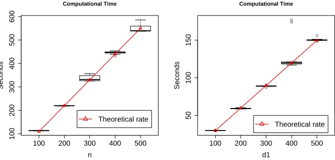
Figure 1: The computational time of our algorithm as the sample size and the tensor di-mension varies. The theoretical linear rate is shown in red triangle.
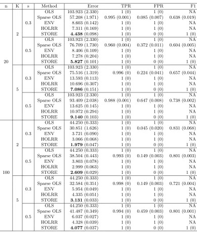
Table 1 reports simulation results based on 20 replications. It is seen that our STORE method clearly achieves a superior performance than all the competing methods in terms of both estimation accuracy and variable selection accuracy. The same pattern holds for different sample sizen, rankK, and sparsity levels. It is also noted that, since OLS, ENV, and HOLRR do not incorporate entry-wise sparsity, their corresponding TPR and FPR values are always one, and their F1 scores are undefined due to zero in the denominator of the precision.
We also studied the computational time of our algorithm when the sample size and the tensor dimension increase. The code is written in R and is implemented on a laptop with 2.5 GHz Intel Core i7 processor. Figure 5.1 reports the results based on 20 replications. Specifically, we fixed the rank K = 2 and the sparsity s = 0.3. In the left panel, we fixed the tensor dimensions d1 = 100, d2 = 50, d3 = 20, but varied the sample size n ∈ {100,200,300,400,500}. In the right panel, we fixed n= 20,d2 = 50, d3 = 20, but varied the dimensiond1∈ {100,200,300,400,500}. This scale of sample size and tensor dimension
is typical in neuroimaging applications. From the plot we see that the computational time of our Algorithm 1 is roughly linear in terms of the sample size and the tensor dimension when other parameters are fixed. This shows that our algorithm is scalable and feasible with moderate to large sample size and dimensionality. Meanwhile, it is possible to further improve our current algorithm. For instance, in each iteration, one could employ the recently developed parallel tensor decomposition (Papalexakis et al., 2012), or the sketching tensor decomposition (Wang et al., 2015), to accelerate the computation.
5.2 2D Symmetric Matrix Response Example
n K s Method Error TPR FPR F1 OLS 103.923 (2.330) 1 (0) 1 (0) NA Sparse OLS 57.208 (1.971) 0.995 (0.001) 0.085 (0.007) 0.638 (0.019) 0.3 ENV 8.603 (0.142) 1 (0) 1 (0) NA HOLRR 7.311 (0.169) 1 (0) 1 (0) NA 2 STORE 4.438(0.098) 1 (0) 0 (0) 1 (0) OLS 103.923 (2.330) 1 (0) 1 (0) NA Sparse OLS 76.709 (1.730) 0.960 (0.004) 0.372 (0.011) 0.604 (0.005) 0.5 ENV 8.406 (0.109) 1 (0) 1 (0) NA HOLRR 7.278 (0.204) 1 (0) 1 (0) NA 20 STORE 5.827(0.101) 1 (0) 0 (0) 1 (0) OLS 103.923 (2.330) 1 (0) 1 (0) NA Sparse OLS 75.516 (1.319) 0.996 (0) 0.224 (0.041) 0.657 (0.044) 0.3 ENV 13.593 (0.113) 1 (0) 1 (0) NA HOLRR 10.696 (0.307) 1 (0) 1 (0) NA 5 STORE 7.086(0.151) 1 (0) 0 (0) 1 (0) OLS 103.923 (2.330) 1 (0) 1 (0) NA Sparse OLS 93.409 (2.038) 0.988 (0.001) 0.647 (0.008) 0.738 (0.002) 0.5 ENV 13.625 (0.145) 1 (0) 1 (0) NA HOLRR 10.972 (0.294) 1 (0) 1 (0) NA STORE 9.140(0.103) 1 (0) 0 (0) 1 (0) OLS 44.250 (0.333) 1 (0) 1 (0) NA Sparse OLS 30.851 (1.626) 1 (0) 0.045 (0.020) 0.831 (0.068) 0.3 ENV 3.721 (0.090) 1 (0) 1 (0) NA HOLRR 3.066 (0.068) 1 (0) 1 (0) NA 2 STORE 1.979(0.047) 1 (0) 0 (0) 1 (0) OLS 44.250 (0.333) 1 (0) 1 (0) NA Sparse OLS 38.504 (0.443) 0.993 (0) 0.149 (0.003) 0.801 (0.003) 0.5 ENV 3.803 (0.078) 1 (0) 1 (0) NA HOLRR 2.999 (0.063) 1 (0) 1 (0) NA 100 STORE 2.609(0.029) 1 (0) 0 (0) 1 (0) OLS 44.250 (0.333) 1 (0) 1 (0) NA Sparse OLS 32.584 (0.351) 0.998 (0) 0.149 (0.003) 0.721 (0.004) 0.3 ENV 5.954 (0.049) 1 (0) 1 (0) NA HOLRR 4.335 (0.051) 1 (0) 1 (0) NA 5 STORE 3.131(0.033) 1 (0) 0 (0) 1 (0) OLS 44.250 (0.333) 1 (0) 1 (0) NA Sparse OLS 41.487 (0.349) 0.994 (0) 0.459 (0.003) 0.801 (0.001) 0.5 ENV 6.037 (0.027) 1 (0) 1 (0) NA HOLRR 4.328 (0.039) 1 (0) 1 (0) NA STORE 4.077(0.037) 1 (0) 0 (0) 1 (0)
Table 1: Third-order tensor response example with different sample size n, rank K, and sparsitys. Reported are the average estimation error, TPR, FPR, and F1 score, with the standard error shown in the parenthesis. The minimal error in each case is shown in boldface.
Graph Pattern Method Estimation Error TPR FPR F1
OLS 22.168 (0.560) 1 (0) 1 (0) NA
Sparse OLS 15.855 (0.543) 1 (0) 0.232 (0.012) 0.646 (0.012)
random ENV 10.751 (0.352) 1 (0) 1 (0) NA
HOLRR 8.318 (0.199) 1 (0) 1 (0) NA
STORE 2.497(0.075) 1 (0) 0 (0) 1 (0)
OLS 22.168 (0.560) 1 (0) 1 (0) NA
Sparse OLS 12.924 (0.197) 0.338 (0.060) 0 (0) 0.443 (0.073)
hub ENV 17.811 (0.222) 1 (0) 1 (0) NA
HOLRR 11.685 (0.110) 1 (0) 1 (0) NA
STORE 7.448(0.453) 0.824 (0.043) 0.079 (0.004) 0.272 (0.010)
OLS 23.481 (0.635) 1 (0) 1 (0) NA
Sparse OLS 22.024 (0.819) 0.821 (0.063) 0.010 (0.001) 0.816 (0.062)
small-world ENV 28.173 (0.427) 1 (0) 1 (0) NA
HOLRR 18.794(0.319) 1 (0) 1 (0) NA
STORE 21.309 (0.154) 0.901 (0.014) 0.118 (0.004) 0.610 (0.002)
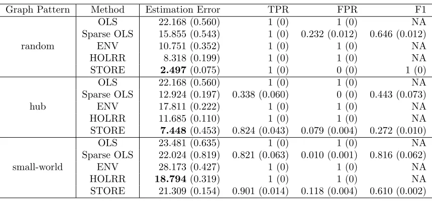
Table 2: Symmetric matrix response example with different graph structures. Reported are the average estimation error, TPR, FPR, and F1 score, with the standard error shown in the parenthesis. The minimal error in each example is shown in boldface.
and a small-world graph (small-world). Note that the coefficient tensor B is symmetric, though the corresponding graph pattern is not necessarily so. The random and hub graphs are both of a low-rank structure, with the true rank K = 2 and K= 10, respectively. The small-world graph is not of an exact low-rank structure, and our method essentially provides a low-rank approximation. This scenario also allows us to investigate the performance of our method under potential model mis-specification. Besides, as none of the competitive solution enforces the symmetry property of the estimatorBb, for comparison, we symmetrized
their final estimators by (Bb+Bb>)/2.
Graph Pattern: True ● ● ● ● ● ● ● ● ● ● ● ● ● ●● ● ● ● ● ● ● ● ● ● ● ● ● ● ● ● ● ● ● ● ● ● ● ● ● ● ● ● ● ● ● ● ● ● ● ● ● ● ● ● ● ● ● ● ● ● ● ● ● ● ● ● ● ● ● ● ● ● ● ● ● ● ● ● ● ● ● ● ● ● ● ● ● ● ● ● ● ● ●● ● ● ● ● ● ●
Graph Pattern: OLS/ENV/HOLRR
● ● ● ● ● ● ● ● ● ● ● ● ● ●● ● ● ● ● ● ● ● ● ● ● ● ● ● ● ● ● ● ● ● ● ● ● ● ● ● ● ● ● ● ● ● ● ● ● ● ● ● ● ● ● ● ● ● ● ● ● ● ● ● ● ● ● ● ● ● ● ● ● ● ● ● ● ● ● ● ● ● ● ● ● ● ● ● ● ● ● ● ●● ● ● ● ● ● ●
Graph Pattern: Sparse OLS
● ● ● ● ● ● ● ● ● ● ● ● ● ●● ● ● ● ● ● ● ● ● ● ● ● ● ● ● ● ● ● ● ● ● ● ● ● ● ● ● ● ● ● ● ● ● ● ● ● ● ● ● ● ● ● ● ● ● ● ● ● ● ● ● ● ● ● ● ● ● ● ● ● ● ● ● ● ● ● ● ● ● ● ● ● ● ● ● ● ● ● ●● ● ● ● ● ● ●
Graph Pattern: STORE
● ● ● ● ● ● ● ● ● ● ● ● ● ●● ● ● ● ● ● ● ● ● ● ● ● ● ● ● ● ● ● ● ● ● ● ● ● ● ● ● ● ● ● ● ● ● ● ● ● ● ● ● ● ● ● ● ● ● ● ● ● ● ● ● ● ● ● ● ● ● ● ● ● ● ● ● ● ● ● ● ● ● ● ● ● ● ● ● ● ● ● ●● ● ● ● ● ● ●
Graph Pattern: True
● ● ● ● ● ● ● ● ● ● ● ● ● ● ● ● ● ● ● ● ● ● ● ● ● ● ● ● ● ● ● ● ● ● ● ● ● ● ● ● ● ● ● ● ● ● ● ● ● ● ● ● ● ● ● ● ● ● ● ● ● ● ● ● ● ● ● ● ● ● ● ● ● ● ● ● ● ● ● ● ● ● ● ● ● ● ● ● ● ● ● ● ● ● ● ● ● ● ● ●
Graph Pattern: OLS/ENV/HOLRR
● ● ● ● ● ● ● ● ● ● ● ● ● ● ● ● ● ● ● ● ● ● ● ● ● ● ● ● ● ● ● ● ● ● ● ● ● ● ● ● ● ● ● ● ● ● ● ● ● ● ● ● ● ● ● ● ● ● ● ● ● ● ● ● ● ● ● ● ● ● ● ● ● ● ● ● ● ● ● ● ● ● ● ● ● ● ● ● ● ● ● ● ● ● ● ● ● ● ● ●
Graph Pattern: Sparse OLS
● ● ● ● ● ● ● ● ● ● ● ● ● ● ● ● ● ● ● ● ● ● ● ● ● ● ● ● ● ● ● ● ● ● ● ● ● ● ● ● ● ● ● ● ● ● ● ● ● ● ● ● ● ● ● ● ● ● ● ● ● ● ● ● ● ● ● ● ● ● ● ● ● ● ● ● ● ● ● ● ● ● ● ● ● ● ● ● ● ● ● ● ● ● ● ● ● ● ● ●
Graph Pattern: STORE
● ● ● ● ● ● ● ● ● ● ● ● ● ● ● ● ● ● ● ● ● ● ● ● ● ● ● ● ● ● ● ● ● ● ● ● ● ● ● ● ● ● ● ● ● ● ● ● ● ● ● ● ● ● ● ● ● ● ● ● ● ● ● ● ● ● ● ● ● ● ● ● ● ● ● ● ● ● ● ● ● ● ● ● ● ● ● ● ● ● ● ● ● ● ● ● ● ● ● ●
Graph Pattern: True
● ● ● ● ● ● ● ● ● ● ● ● ● ● ● ● ● ● ● ● ● ● ●● ● ● ●● ● ● ● ● ● ● ● ● ● ● ● ● ● ● ● ● ● ● ● ● ● ● ● ● ● ● ● ● ● ●● ● ● ● ● ● ● ● ● ● ● ● ● ● ● ● ● ● ● ● ● ●● ● ● ● ● ● ● ● ● ● ● ● ● ● ● ● ● ● ● ●
Graph Pattern: OLS/ENV/HOLRR
● ● ● ● ● ● ● ● ● ● ● ● ● ● ● ● ● ● ● ● ● ● ●● ● ● ●● ● ● ● ● ● ● ● ● ● ● ● ● ● ● ● ● ● ● ● ● ● ● ● ● ● ● ● ● ● ●● ● ● ● ● ● ● ● ● ● ● ● ● ● ● ● ● ● ● ● ● ●● ● ● ● ● ● ● ● ● ● ● ● ● ● ● ● ● ● ● ●
Graph Pattern: Sparse OLS
● ● ● ● ● ● ● ● ● ● ● ● ● ● ● ● ● ● ● ● ● ● ●● ● ● ●● ● ● ● ● ● ● ● ● ● ● ● ● ● ● ● ● ● ● ● ● ● ● ● ● ● ● ● ● ● ●● ● ● ● ● ● ● ● ● ● ● ● ● ● ● ● ● ● ● ● ● ●● ● ● ● ● ● ● ● ● ● ● ● ● ● ● ● ● ● ● ●
Graph Pattern: STORE
● ● ● ● ● ● ● ● ● ● ● ● ● ● ● ● ● ● ● ● ● ● ●● ● ● ●● ● ● ● ● ● ● ● ● ● ● ● ● ● ● ● ● ● ● ● ● ● ● ● ● ● ● ● ● ● ●● ● ● ● ● ● ● ● ● ● ● ● ● ● ● ● ● ● ● ● ● ●● ● ● ● ● ● ● ● ● ● ● ● ● ● ● ● ● ● ● ●
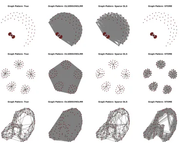
Figure 2: Symmetric matrix response example. Top row: the random graph, middle row: the hub graph, bottom row: the small-world graph. The first column: the true graph pattern; The second column: the estimated graph from OLS, ENV, and HOLRR; The third column: the estimated graph from Sparse OLS; The forth column: the estimated graph from our method STORE.
example, its graph estimate is completely dense and the corresponding FPR is one. Sparse OLS recoveres the graph pattern reasonably well, but still misses many true positive links, and yields a smaller TPR than our method.
6. Real Data Analysis
functional magnetic resonance imaging (fMRI) of 795 subjects, of which 362 have ASD, and 433 are the normal controls. We took the fMRI image as the response, and the ASD status indicator (1 = ASD and 0 = normal control), age and sex as covariates. For each fMRI image, there are two forms of data: one is a 3D tensor and another is a 2D symmetric matrix. Correspondingly, we have fitted two separate tensor response regression models.
6.1 3D FALFF Tensor Response
The first form of the fMRI data is a third-order tensor of fractional amplitude of low-frequency fluctuations (fALFF). fALFF is a metric reflecting the percentage of power spec-trum within low-frequency domain (0.01−0.1 Hz). It characterizes the intensity of sponta-neous brain activities, and provides a measure of functional architecture of the brain (Shi and Kang, 2015). It is calculated at each individual image voxel, and forms a 3D tensor with dimension 91×109×91. We applied our STORE method as well as four competing methods (OLS, Sparse OLS, ENV, and HOLRR) to this general 3D tensor response.
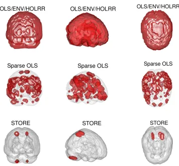
Figure 3 shows the estimated coefficient tensors, overlaid on a brain image of a randomly selected subject, by all five methods. Among those, OLS, ENV, and HOLRR perform no region selection, whereas Sparse OLS yields a sparse estimate that is difficult to interpret. By contrast, the STORE estimate reveals a small number of brain regions that exhibit a clear difference between the ASD and normal control groups. Furthermore, we mapped those nonzero entries of our estimate to the AAL atlas. Table 3 reports the names of those identified regions and the corresponding coefficient entries in each region. Our results in general agree with the autism literature. For instance, we have found that multiple cerebel-lum (Cerebellum) regions show distinctive patterns between the ASD and control groups. The cerebellum has long been known for its importance in motor learning, coordination, and more recently, cognitive functions and affective regulation. It has emerged as one of the key brain regions affected in autism (Becker and Stoodley, 2013). Moreover, we identified the superior parietal lobule (Parietal Sup) and precuneus (Precuneus), which agrees with Travers et al. (2015), in that they found individuals with ASD showed decreased activation in the superior parietal lobule and precuneus relative to individuals with typical develop-ment, suggesting that the superior parietal lobule may play an important role in motor learning and repetitive behavior in individuals with ASD.
6.2 2D Symmetric Partial Correlation Matrix Response
Figure 3: Analysis of the ABIDE data. The response is a 3D brain image tensor. Shown are the estimated coefficient tensor overlaid on a randomly selected brain image. Top row: OLS/ENV/HOLRR, middle row: Sparse OLS, bottom row: STORE. Left column: front view, middle column: side view, right column: top view.
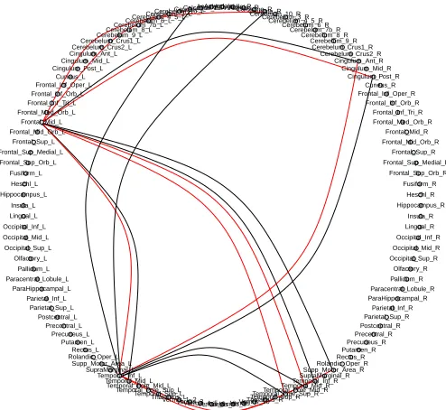
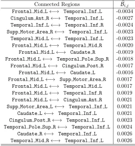
Figure 4 reports top 20 identified links from our method. The red links correspond to those that are more likely to be absent in the ASD group, whereas the black ones are those more likely to be present in ASD. Table 4 reports the names of those links and their relative connection strengthens in the network, as reflected by the corresponding entries in the matrix coefficient Bb. Many different connectivity patterns concentrate on the left
middle frontal gyrus (Frontal Mid L) and the temporal lobe (Temporal), and such findings again agrees with the literature (Kana et al., 2006; Di Martino et al., 2014; Ha et al., 2015).
Acknowledgments
Important Regions Bbi,j,k
Postcentral L 0.0033
Cerebelum 9 L 0.0028
Precuneus L 0.0025
Occipital Sup R 0.0025
Parietal Inf L 0.0025
Cerebelum 8 L 0.0020
Cerebelum 8 R 0.0020
Precuneus R 0.0017
Parietal Sup R 0.0017
Cerebelum 9 R 0.0016
Parietal Sup L 0.0016
Table 3: Analysis of the ABIDE data. The response is the third-order fALFF tensor. Re-ported are the identified brain regions by our method that exhibit clear difference in fALFF between the ASD and normal control.
● ● ● ● ● ● ● ● ● ● ● ● ● ● ● ● ● ● ● ● ● ● ● ● ● ● ● ● ● ● ● ● ● ● ● ● ● ● ● ● ●● ● ● ● ● ● ● ● ● ● ● ● ● ● ● ● ● ● ● ● ● ● ● ● ● ● ● ● ● ● ● ● ● ● ● ● ● ● ● ● ● ● ● ● ● ● ● ● ● ● ● ● ● ● ● ● ● ● ● ● ● ● ● ● ● ● ● ●●●●●●●● Precentral_L Precentral_R Frontal_Sup_L Frontal_Sup_R Frontal_Sup_Orb_L Frontal_Sup_Orb_R Frontal_Mid_L Frontal_Mid_R Frontal_Mid_Orb_L Frontal_Mid_Orb_R Frontal_Inf_Oper_L Frontal_Inf_Oper_R Frontal_Inf_Tri_L Frontal_Inf_Tri_R Frontal_Inf_Orb_L Frontal_Inf_Orb_R Rolandic_Oper_L Rolandic_Oper_R Supp_Motor_Area_L Supp_Motor_Area_R Olfactory_L Olfactory_R Frontal_Sup_Medial_L Frontal_Sup_Medial_R Frontal_Med_Orb_L Frontal_Med_Orb_R Rectus_L Rectus_R Insula_L Insula_R Cingulum_Ant_L Cingulum_Ant_R Cingulum_Mid_L Cingulum_Mid_R Cingulum_Post_L Cingulum_Post_R Hippocampus_L Hippocampus_R ParaHippocampal_L ParaHippocampal_R Amygdala_LAmygdala_R Calcarine_L Calcarine_R Cuneus_L Cuneus_R Lingual_L Lingual_R Occipital_Sup_L Occipital_Sup_R Occipital_Mid_L Occipital_Mid_R Occipital_Inf_L Occipital_Inf_R Fusiform_L Fusiform_R Postcentral_L Postcentral_R Parietal_Sup_L Parietal_Sup_R Parietal_Inf_L Parietal_Inf_R SupraMarginal_L SupraMarginal_R Angular_L Angular_R Precuneus_L Precuneus_R Paracentral_Lobule_L Paracentral_Lobule_R Caudate_L Caudate_R Putamen_L Putamen_R Pallidum_L Pallidum_R Thalamus_L Thalamus_R Heschl_L Heschl_R Temporal_Sup_L Temporal_Sup_R Temporal_Pole_Sup_L Temporal_Pole_Sup_R Temporal_Mid_L Temporal_Mid_R Temporal_Pole_Mid_L Temporal_Pole_Mid_R Temporal_Inf_L Temporal_Inf_R Cerebelum_Crus1_L Cerebelum_Crus1_R Cerebelum_Crus2_L Cerebelum_Crus2_R Cerebelum_3_L Cerebelum_3_R Cerebelum_4_5_L Cerebelum_4_5_R Cerebelum_6_L Cerebelum_6_R Cerebelum_7b_L Cerebelum_7b_R Cerebelum_8_L Cerebelum_8_R Cerebelum_9_L Cerebelum_9_R Cerebelum_10_L Cerebelum_10_R
Vermis_1_2Vermis_3Vermis_4_5Vermis_6 Vermis_7Vermis_9 Vermis_10Vermis_8
Connected Regions Bbi,j
Frontal Mid L←→ Temporal Inf L -0.0034
Cingulum Ant R←→ Temporal Inf L -0.0027
Temporal Inf L←→ Temporal Inf R -0.0024
Supp Motor Area R←→ Temporal Inf L -0.0023
Temporal Mid L←→ Temporal Inf L -0.0023
Frontal Mid L←→ Temporal Mid R -0.0020
Frontal Mid L←→ Caudate R -0.0019
Frontal Mid L←→ Temporal Pole Sup R -0.0018
Frontal Mid L←→ Cingulum Post R -0.0017
Frontal Mid L←→ Caudate L -0.0016
Frontal Mid L←→ Supp Motor Area R 0.0017
Frontal Mid L←→ Temporal Mid L 0.0017
Frontal Mid L←→ Temporal Inf R 0.0019
Frontal Mid L←→ Cingulum Ant R 0.0021
Supp Motor Area L←→ Temporal Inf L 0.0021
Caudate L←→ Temporal Inf L 0.0021
Cingulum Post R←→ Temporal Inf L 0.0023
Temporal Pole Sup R←→ Temporal Inf L 0.0024
Caudate R←→ Temporal Inf L 0.0026
Temporal Mid R←→ Temporal Inf L 0.0026
Appendix A.
We divide the appendix into three parts. First we begin with a number of auxiliary lemmas. Next we provide detailed proofs of the main theorem. Then we present the technical proofs of all lemmas and corollaries.
A1 Auxiliary Lemmas
Lemma 9 For any matrix Yi ∈Rd1×d2, with i= 1, . . . , n, and vectorsγ = (γ1, . . . , γn)>∈
Rn, α∈Rd1 and β∈Rd2, we have
arg min β,kβk2=1
1
n
n
X
i=1 γ2i
Yi−αβ
> 2
F = argβ,kminβk2=1
1
n
n
X
i=1
γi2Yi−αβ>
2
F.
The proof of Lemma 9 is provided in Section A3.3 in the online supplement.
We next introduce the Slepian’s lemma (Slepian, 1962), which provides a comparison between the supremums of two Gaussian processes.
Lemma 10 (Slepian, 1962, Slepian’s Lemma) Denote two centered Gaussian processes {Gs, s∈ S}and{Hs, s∈ S}. Assume that both processes are almost surely bounded and for
each s, t∈ S, E(Gs−Gt)2 ≤E(Hs−Ht)2, then we have
E
sup s∈S
Gs
≤E
sup s∈S
Hs
.
Moreover, if E(G2s) =E(Hs2) for alls∈ S, then we have, for each x >0,
P
sup s∈S
Gs> x
≤P
sup s∈S
Hs> x
.
The next result provides a concentration of Lipschitz functions of Gaussian random variables (Massart, 2003) .
Lemma 11 (Massart, 2003, Theorem 3.4) Letv∈Rd be a Gaussian random variable such
thatv∼N(0,Id). Assumingg(v)∈Rto be a Lipschitz function such that|g(v1)−g(v2)| ≤ Lkv1−v2k2 for anyv1,v2 ∈Rd, then we have, for each t >0,
P[|g(v)−E[g(v)]| ≥t]≤2 exp
− t 2
2L2
.
The next lemma provides an upper bound of the Gaussian width of the unit ball for the sparsity regularizer (Raskutti and Yuan, 2016).
Lemma 12 (Raskutti and Yuan, 2016, Lemma 2) For a tensor T ∈ Rd1×d2×d3, denote
its regularizer R(T) = P
j1
P
j2
P
j3|Tj1,j2,j3|. Define the unit ball of this regularizer as
BR(1) :={T ∈Rd1×d2×d3|R(T) ≤1}. For a Gaussian tensor G ∈Rd1×d2×d3 whose entries are independent standard normal random variables, we have
E "
sup
T ∈BR(1)
hT,Gi #
The next lemma links the hard thresholding sparsity and the L1-penalized sparsity. Lemma 13 For any vectors u∈Rd1,v∈
Rd2,w∈Rd3 satisfying kuk2 =kvk2 =kwk2 =
1,kuk0 ≤ s,kvk0 ≤ s, and kwk0 ≤s, denoting A:= u◦v◦w, we have the bound of the L1-norm regularizer
kAk1 := X
j1
X
j2
X
j3
|Aj1j2j3| ≤s
3/2.
A2 Proof of Theorem 6
We divide the proof of Theorem 6 into two major steps: characterization of the estimation error in Step 1 in Algorithm 1, then the estimation error in Step 2. Each leads to a new theorem. Then we complete the proof of Theorem 6 by iteratively applying those results.
A2.1 Estimation Error in Step 1 of Algorithm 1
We first derive the estimation error in Step 1 of our Algorithm 1. The key idea is to transform the problem into a standard sparse tensor decomposition problem, then incorporate the existing contracting results obtained in Sun et al. (2017) to derive the final error bound of the estimator in Step 1. In the following derivation, for simplicity, we assumeK = 1. This does not lose generality, sinceKis assumed to be a constant, and it does not affect the final error rate. In this case, the true model reduces to Yi =w∗(β∗>k,m+1xi)βk,∗1◦ · · · ◦βk,m∗ +Ei, for eachi= 1, . . . , n. Based on the Step 1 of our algorithm, if the true parameterβk,m∗ +1 is available, we are solving the following sparse tensor decomposition problem,
¯
Rk =T + ¯E, (A1)
where the true tensor T =wk∗β∗k,1◦ · · · ◦βk,m∗ , the oracle response and the oracle error are, respectively,
¯ Rk := 1
n
n
X
i=1
Rik= 1
n
n
X
i=1 Yi
β∗>k,m+1xi
and ¯E = 1
n
n
X
i=1 Ei
βk,m∗>+1xi
.
In practice, however, we only have an estimatorβbk,m+1. Hence the sparse tensor
decompo-sition method in Step 1 of our algorithm is actually applied to
b
Rk=T +Eb (A2)
with the response tensor
b Rk:= 1
n
n
X
i=1 Yi
b
β>k,m+1xi
Therefore, according to (A1) and (A2), we have the explicit form ofEb,
b
E = Rbk−R¯k+ ¯E
= 1
n
n
X
i=1
(β∗k,m+1−βbk,m+1)>xi b
β>k,m+1xiβk,m∗>+1xi
Yi
| {z }
I1
+1
n
n
X
i=1 Ei
βk,m∗>+1xi
| {z }
I2
Before we derive the estimation error of the estimator based on (A2), we introduce a lemma for deriving the error bound of a general sparse tensor decomposition.
Assumption 14 The decomposition components are incoherent such that
ζ := max i6=j {|hβ
∗
i,1,βj,∗1i|,|hβi,∗2,βj,∗2i|,|hβ∗i,3,β∗j,3i|} ≤ C0 √
d0 ,
withd0 = max{d01, d02, d03}, and for anyj,kPi6=jwihβi,∗1,βj,∗1ihβ∗i,2,βj,∗2iβi,∗3k ≤C1w∗max √
Kζ. Moreover, the matricesA:= [βi,∗1,· · · ,βK,∗ 1],B:= [β∗i,2,· · · ,β∗K,2], andC:= [β∗i,3,· · ·,βK,∗ 3]
satisfy thatmax{kAk,kBk,kCk} ≤1 +C2pK/d0 for some positive constants C0, C1, C2.
Define a function f(;K, d0) as
f(;K, d0) :=
2C0 √
d0
1 +C2 r
K d0
2 +C1
√ K d0
+C32,
for some constantsC0, C1, C2, C3 >0. When K=o(d03/2), the first two terms of f(;K, d0) converge to 0 and the last term is the contracting term.
Lemma 15 (Sun et al., 2017, Lemma S.4.1) Consider the model Tb = T +E where the low-rank and sparse components of T satisfy Assumption 14, and assume kT k ≤ C3w∗max and K=o(d03/2). In addition, assume the estimators βbj,1 and βbj,2 satisfy D(βbj,1,βj,∗1)≤ and D(βbj,2,βj,∗2)≤for some j ∈[K]. If the perturbation error η(E, d0+s), with s≥d0, is small enough such that η(E, d0+s)< wj(1−2)−w∗maxf(;K, d0), then the updateβbj,3 satisfies, with high probability,
D(βbj,3,βj,∗3)≤ √
5wmax∗ f(;K, d0) +√5η(E, d0+s)
wj(1−2)−w∗maxf(;K, d0)−η(E, d0+s) .
If we further assumeD(βbj,3,βj,∗3)≤, then the updatewb=T ×b 1βbj,1×2βbj,2×3βbj,3 satisfies, with high probability, |wb−wj| ≤2wj2+w∗maxf(;K, d0) +η(E, d0+s).
By verifying the conditions in Lemma 15, we are able to compute the estimation error in Step 1 of our algorithm. For simplicity, we consider the case when m = 3, while the extension to a more generalm is straightforward.
Lemma 16 Assume kT k ≤C1w∗max, D(βbk,1,βk,∗1)≤, D(βbk,2,β∗k,2)≤, and
<min
(s
w∗min
2(wmin∗ +wmax∗ C1),
w∗min
4√5wmax∗ C1 )
.
Assume the error tensor satisfies η(Eb, d0+s)≤w∗min/4 with s≥d0, whereEbis as defined in (A3). Then we have
D(βbk,3,βk,∗3)≤κ1+
4√5
where the contraction coefficient
κ1:= 4 √
5w∗maxC1 wmin∗ <
4√5w∗maxC1 wmin∗ min
(s
wmin∗
2(w∗min+w∗
maxC1)
, w
∗
min
4√5w∗
maxC1 )
∈(0,1).
The proof of Lemma 16 is provided in Section A3.5. Based on Lemma 16, to compute the closed-form error rate in Step 1 of our Algorithm, the remaining step is to compute
η(Eb, s), since η(Eb, d0+s) ≤2η(Eb, s) by noting that s≥d0. Here the explicit form of Ebis
defined in (A3). Again we only consider m = 3 for simplicity, and the proof for a general
m follows straightforwardly.
Lemma 17 Assume the conditions in Lemma 16 hold. Assume thatkwk∗β∗k,1◦ · · · ◦βk,m∗ k ≤ C1, kxik ≤ C2, and |βk,m∗>+1xi| ≥ C3 for each i = 1, . . . , n, for some positive constants C1, C2, C3. If ≤C3/(2C2), then we have
η(Eb, s)≤
2C2η E¯, s C32 | {z }
κ2
+ 1
C3
η E¯, s .
where E¯:= n1 Pn
i=1Ei.
The proof of Lemma 17 is provided in Section A3.6. Combining Lemma 16 and Lemma 17, we obtain the final contraction result of Step 1 in Algorithm 1.
Theorem 18 (Contraction result in Step 1 in Algorithm 1) Assume D(βbk,1,βk,∗1) ≤ , D(βbk,2,β∗k,2)≤, and D(βbk,4,β∗k,4)≤, with
<min
(s
w∗min
2(w∗min+w∗
maxC1)
, w
∗
min
4√5wmax∗ C1, C3
2C2 )
.
Assume the error tensor satisfies η(n−1Pn
i=1Ei, d0 +s) ≤ w∗min/4 with s ≥ d0. Then we have
D(βbk,3,βk,∗3)≤(κ1+κ2)+
4√5
C3w∗min η 1
n
n
X
i=1 Ei, s
! .
A2.2 Estimation Error in Step 2 of Algorithm 1
Next we derive the estimation error in Step 2 of our algorithm. That is, we aim to bound
D(βbk,m+1,β∗k,m+1) given the estimators b
wk,βbk,1, . . . ,βbk,m.
DenoteAbk=wbkβbk,1◦· · ·◦βbk,m, andTbi =Yi− P
k06=k,k0∈[K]wbk0(βb>k0,m+1xi)βbk0,1◦· · ·◦βbk0,m,
and the closed-form estimator in Step 2 of our algorithm is
b
βk,m+1 =
1
n
n
X
i=1 xix>i
!−1
n−1Pn
i=1hTbi,Abkixi kAbkk2F
Theorem 19 (Contraction result in Step 2 in Algorithm 1) Under Assumption 3, and the assumption that the initialization error satisfies≤w∗min/2, if|wbk−w∗k| ≤,D(βbk,1,β∗k,1)≤ , . . . , D(βbk,m,β∗k,m)≤, then we have
D(βbk,m+1,βk,m∗ +1)≤κ3+ e C √
n,
where κ3:= 2/wmin∗ + 6√2 and Ce is a positive constant as defined in (A7).
Proof: For simplicity, we only prove forK = 1 andm= 3. The derivation for a general
K andm follows similarly.
Denote A∗k := w∗kβk,∗1 ◦ βk,∗2 ◦ βk,∗3. The true model reduces to Yi = (βk,∗>4xi)A∗k +
Ei, for each i= 1, . . . , n.Denote Ω := (n−1Pni=1xix>i )−1. GivenAbk =wbkβbk,1◦ · · · ◦βbk,3,
and Tbi=Yi when K= 1, we have the following simplification of βbk,4,
b
βk,4 = Ω Pn
i=1hTbi,Abkixi nkAbkk2F
= Ω
Pn
i=1h(β∗>k,4xi)A∗k+Ei,Abkixi
nkAbkk2F
= hA
∗
k,Abki kAbkk2F
βk,∗4+Ω
Pn
i=1hEi,Abkixi nkAbkk2F
, (A4)
where the first part in (A4) is due to the fact thatn−1Pn
i=1(β
∗>
k,4xi)Ωxi =n
−1Pn
i=1Ωxix
>
i β
∗
k,4 =
β∗k,4. Therefore, the error bound of βbk,4 can be simplified as
βbk,4−β
∗
k,4
2 =
hA∗
k,Abki kAbkk2F
β∗k,4−βk,∗4+Ω
Pn
i=1hEi,Abkixi nkAbkk2F
2
,
≤
hA∗
k,Abki − kAbkk2F kAbkk2F
| {z }
(I)
+kΩ
Pn
i=1hEi,Abkixik2 nkAbkk2F | {z }
(II)
. (A5)
In the following lemma, we bound the two terms in (A5) to obtain the final error bound.
Lemma 20 Under the Conditions in Theorem 19, we have
(I) ≤
2
w∗min + 6 √
2
, (A6)
(II) ≤ maxikΩxik2·E[kGkF] kAbkkF
| {z }
e
C
·√1
n. (A7)
Finally, combining the results in (A6) and (A7) leads to the final bound of kβbk,4−β∗k,4k2,
A2.3 Proof of Theorem 6
Now we complete the proof of Theorem 6, by iteratively applying the contraction results in Theorems 18 and 19 for the two steps of Algorithm 1. In iteration t = 1, given the initializations βb
(0)
k,j and wb
(0) with initialization error , Theorem 18 implies that
D(βb (1)
k,3,β
∗
k,3)≤(κ1+κ2)+
4√5
C3w∗min η 1
n
n
X
i=1 Ei, s
! ,
whereκ1+κ2<1 according to Assumptions 4 and 5. The second term converges to zero as
sample size increases. Therefore, for a sufficiently large sample size, the above error bound is smaller than . By a similar derivation, the same error bound holds for D(βb
(1)
k,1,β
∗
k,1), D(βb
(1)
k,2,β
∗
k,2), and |wb (1)
k −w
∗
k|. In Step 2 of the algorithm, applying Theorem 19 based on the above estimators in iterationt= 1, we obtain that
D(βb (1)
k,4,β
∗
k,4)≤κ3(κ1+κ2)+κ3
4√5
C3wmin∗ η 1
n
n
X
i=1 Ei, s
!
+√Ce n.
Again, the contraction coefficient κ3(κ1+κ2) <1 according to Assumptions 4 and 5, and
the remaining term converges to zero as sample size increases. Forκ= (κ1+κ2)κ3 ∈(0,1), by repeatedly applying these derivations, in the titeration, we obtain that
max
max k kwb
(t)
k −w
∗
kk2,max k,j
kβb
(t)
k,j−β
∗
k,jk2
≤ κt+1−κ t
1−κ
4√5
C3wmin∗ η
1
n
n
X
i=1 Ei, s
!
+1−κ t−1
1−κ e C √
n
≤ κt+ 1 1−κmax
(
4√5
C3wmin∗ η
1
n
n
X
i=1 Ei, s
! ,√Ce
n )
.
This completes the proof of Theorem 6.
A3 Proofs of Lemmas and Corollaries
This subsection provides all the supporting lemmas and corollaries as well as their proofs.
A3.1 Proof of Lemma 1
To solve (4), we can use the alternating updating method to update one parameter at a time. In particular, for eachj= 1, . . . , m, given βk(j0) with j0 6=j, we solve
b
βk,j := arg min βk,j
kβk,jk2=1,kβk,jk0≤sj
1
n
n
X
i=1 α2ik
Ri−wkβk,1◦ · · · ◦βk,m 2
F.
According to the matrix representation of tensor operations (Kolda and Bader, 2009; Kim et al., 2014), this optimization problem is equivalent to solve
min βk,j
kβk,jk2=1,kβk,jk0≤sj
1
n
n
X
i=1 α2ik
[Ri]
>
(j)−h (j)
k β
(j)>
k
2