Solving Multi-objective Linear Bilevel
Multi-follower Programming Problem
E. Ansari ∗, H. Zhiani Rezai
Department of Mathematics, Islamic Azad University, Mashhad branch, Mashhad, Iran Received 19 February 2011; revised 30 October 2011; accepted 8 November 2011.
———————————————————————————————-Abstract
In sciences and industries such as signal optimization, traffic assignment, economic mar-ket and etc, many problems have been modeled by bilevel programming (BLP) problems, where in each level one must optimize some objective functions. There are so many algo-rithms in order to find the global optimum of the linear version of BLP problems.
This paper addresses multi-objective linear bilevel multi-follower programming (MOLBMFP) problems in which there is no sharing information among followers. It presents a new method for solving these problems.
Keywords: Bilvel programming; Multi-objective linear bilevel multi-follower programming; Fuzzy set theory; Fuzzy programming;Kth-best algorithm.
————————————————————————————————–
1
Introduction
A bilevel programming (BLP) problem can be considered as the noncooperative, two-player game, which was first presented by Von Stackelberg [15]. In a basic BLP model, the control for the decision variables is partitioned amongst the players who seek to optimize their individual objective functions. The upper level is called the leader and the lower level is termed as the follower. The game which is said to be ”static” implies that each player has only one move. The leader goes first and attempts to optimize his objective function, then the follower reacts in a way that is personally without regard to extramural effects by observing the leader’s decision.
There are some methods for finding the global optimum of a bilevel programming problem in which only one leader and a follower are involved and each level has just one objective function to be optimized. The majority of researches on bilevel programming problems have been centered on the linear version of the problems, and there have been nearly two dozen algorithms proposed for solving BLP problems [1, 2, 5, 6, 7]. Some of them are:
Penalty function approach [12, 16], Genetic algorithm [10, 11], Grid-search algorithm [2] and theKth-best algorithm [3, 4, 13].
If the feasible region of every linear BLP problem is nonempty and compact, it shares an important property that at least one optimal (global) solution is attained at an extreme point of the constraint region [12]. TheKth-best method computes the global solution of linear BLP problems by enumerating the extreme points of the constraint region.
Our previous work presented a new approach to solve multi-objective linear bilevel pro-gramming problems [9]. this paper is aimed at presenting a method for solving multi-objective linear bilevel multi-follower programming problems. in section 2, we apply Fuzzy set theory and Fuzzy programming which was introduced by Zimmerman [17, 18] to con-vert our problem to a linear bilevel multi-follower programming (LBLMFP) problem. we express theoretical properties of LBLMFP problem in section 3, and it develops theK th-best method, to find the global optimum solution of the achieved LBLMFP problem in section 4. A numerical example is illustrated in section 5 to show the efficiency of the new approach. We the conclusion is presented in section 6.
2
Converting the multi-objective linear bilevel programming
problem to LBLMFP problem
Consider the model of the MOLBLMFP problem in general as it follows, in whichk(k≥2) followers are involved and there is no sharing information among them except the leader’s.
max
x∈X {F1(x, y1, y2, . . . , yk), F2(x, y1, y2, . . . , yk), . . . , Fp(x, y1, y2, . . . , yk)}
s.t Ax+ k ∑
t=1
Btyt≤b
max yi∈Yi
{f1i(x, yi), f2i(x, yi), . . . , fji(x, yi)}
s.t Alix+Cliyi≤bli
(2.1)
where x ∈ X ⊂ ℜn, yi ∈ Yi ⊂ ℜmi, Fr : X×Y1 ×. . .×Yk → ℜ1, fli : X ×Yi → ℜ1,
i = 1, . . . , k, r = 1, . . . , p, l = 1, . . . , j (p, j are the number of the objective functions which must be optimized respectively by the leader and the followers.)and A, Bt, Ali, Cli are appropriate technology matrices. As there is no sharing variables among the followers, all followers have individual objective functions and constraints.
region of the leader and the followers is nonempty and compact.
(LP)r max
x∈X Fr(x, y1, y2, . . . , yk) (r = 1, . . . , p)
s.t Ax+ k ∑
t=1
Btyt≤b
(2.2)
(LP)l max
yi∈Yi
fli(x, yi) (l= 1, . . . , j)
s.t Alix+Cliyi≤bli
(2.3)
Let (x[1]∗, y[1]1 ∗, . . . , yk[1]∗), . . . ,(x[p]∗, y[1p]∗, . . . , yk[p]∗) be the solutions of (2.2). Matrix A is defined as follows:
A=
F1(x[1]∗, y [1]∗ 1 , . . . , y
[1]∗
k ) F2(x[1]∗, y [1]∗ 1 , . . . , y
[1]∗
k ) . . . Fp(x[1]∗, y
[1]∗ 1 , . . . , y
[1]∗
k )
F1(x[2]∗, y [2]∗ 1 , . . . , y
[2]∗
k ) F2(x[2]∗, y [2]∗ 1 , . . . , y
[2]∗
k ) . . . Fp(x[2]∗, y
[2]∗ 1 , . . . , y
[2]∗
k ) ..
. ... . .. ...
F1(x[p]∗, y[1p]∗, . . . , y [p]∗
k ) F2(x[p]∗, y1[p]∗, . . . , y [p]∗
k ) . . . Fp(x[p]∗, y1[p]∗, . . . , y [p]∗
k )
The maximum and minimum values in each column of A are shown by ZrU and ZrL,(r = 1, . . . , p), respectively. The differenceZrU −ZrL is the constants of admissible violations. Now we can define a membership function corresponding to each level (the leader and the followers) for any Fuzzy goal, as the following:
forr= 1, . . . , p
µr(Fr) =
1 Fr(x, y1, . . . , yk)≥ZrU
Fr(x,y1,...,yk)−ZrL ZU
r −ZrL Z l
r≤Fr(x, y1, . . . , yk)−ZrL≤ZrU
0 Fr(x, y1, . . . , yk)−ZrL≤ZrL
(2.4)
One must also follow the above process for the followers (by considering (2.3)) thus the upper and lower bounds of the followers’ objective functions can be denoted byzliU andzLli
fori= 1, . . . , kandl= 1, . . . , l, also the membership functions of the followers are defined as above and are denoted by ϕi(fli(x, yi)) for i =, . . . , k, l = 1, . . . , j. Since membership functions are the degrees of satisfaction, they must be maximized. So if we consider
λ = min{µ1, . . . , µp} and λi = min{ϕ1, . . . , ϕk},where i = 1, . . . , k is the number of the followers, then the MOLBLMFP problem (2.1) changes to the LBLMFP problem (2.5) as follows:
max x∈X,λ λ
s.t Ax+∑kt=1Btyt≤b
µr(Fr)≥λ, r= 1, . . . , p
0≤λ≤1
max yi∈Yi,λi
λi
s.t Alix+Cliyi ≤bli
ϕi(fli(x, yi))≥λi, l= 1, . . . , j
0≤λi≤1
By substituting the membership functions from (2.4) to (2.5), the LBLMFP problem (2.5) changes to:
max x∈X,λ λ
s.t Ax+∑kt=1Btyt≤b
Fr(x, y1, . . . , yk)−(ZrU−ZrL)λ≥ZrL, r= 1, . . . , p
0≤λ≤1
max yi∈Yi,λi
λi
s.t Alix+Cliyi ≤bli
fli(x, yi)−(zliU−zliL)λi ≥zliL, l= 1, . . . , j, i= 1, . . . , k
0≤λi ≤1
(2.6)
Now we have a LBLMFP problem, in which, x∈ X ⊂ ℜn and λ∈ [0,1] are the decision variables for the leader andyi ∈Yi ⊂ ℜmi and λi ∈[0,1] for i= 1, . . . , k are the decision variables for the followers.
3
Theoretical properties of LBLMFP problem
The Kth-best algorithm is aimed at investigating the constraint region of the LBLP problem to find the optimal solution at a vertex of the constraint region. Now we explore the definitions expressed in [12, 13] for the LBLMFP problem (2.6).
Constraint region of the linear BLMFP problem (2.6) is defined as follows:
S={(x, y1, . . . , yk, λ, λi)|Ax+ k ∑
t=1
Btyt≤b, Fr(x, y1, . . . , yk)−(ZrU−ZrL)λ≥ZrL,
Alix+Cliyi ≤bli, fli(x, yi)−(zliU−zliL)λi ≥zliL,0≤λ≤1, 0≤, λi ≤1, i= 1, . . . , k, l= 1, . . . , j, r= 1, . . . , p}
Denote the projection of S onto the leader’s decision space by S(X) and the feasible set for each follower for all (x, λ)∈S(X), these two sets are defined as follows:
S(X) ={(x, λ)|x∈X, λ∈[0,1] :∃yi∈Yi,∃λi ∈[0,1],(x, y1, . . . , yk, λ, λi)∈S, i= 1, . . . , k} (Constraints of the leader and the followers are satisfied.)
Si(x) ={yi∈Yi, λi ∈[0,1] : (x, y1, . . . , yk, λ, λi)∈S, i= 1, . . . , k}
Now we define for each follower, the rational reaction set for any (x, λ) ∈ S(X) as the following:
Pi(x) ={yi ∈Yi, λi∈[0,1] : (yi, λi)∈argmin[λi: (yi, λi)∈Si(x)], i= 1, . . . , k}
Pi(x) is equivalent to the set of the solutions of the following problem for any (x, λ)∈S(X) and i= 1,2, . . . , k:
max yi∈Yi,λi
λi
s.t Ax+
k ∑
t=1
Btyt≤b
Fr(x, y1, . . . , yk)−(ZrU−ZrL)λ≥ZrL, r= 1, . . . , p
0≤λ≤1
Alix+Cliyi ≤bli
fli(x, yi)−(zliU−zliL)λi ≥zliL, l= 1, . . . , j, i= 1, . . . , k
0≤λi ≤1
(3.7)
The followers selectyi andλi from their objective functions by considering the leader’s action. Now we present the Inducible Region of the problem (2.6) by:
IR={(x, y1, . . . , yk, λ, λi) :∈(x, y1, . . . , yk, λ, λi)∈S,(yi, λi)∈Pi(x), i= 1, . . . , k} To ensure that (2.6) has an optimal solution, the following assumptions must be considered:
(i) S is nonempty and compact.
(ii) Pi(x) is nonempty,(i.e. Pi(x)̸=∅).
(iii) Pi(x), is a point to point map from S(X) to Ki which Ki ⊆ Si(x)(otherwise some difficulties may appear, which are explained in [2, 8]).
Thus in terms of the above definitions and notations, the LBLMFP problem (2.6) can be written as [14]:
Theorem 3.1. IfS is nonempty and compact, there exists an optimal solution for a linear BLMFP problem.
Proof: SinceSis nonempty and compact, there exists a point (x∗, y1∗, . . . , yk∗, λ∗, λ∗i)∈
S. Then by the definition of the projection ofS onto the leader’s decision space, we have
(x∗, λ∗)∈S(X)̸=∅
Consequently by the definition of the feasible set for each follower Si(x∗) ̸= ∅. Also by the definition of each follower’s rational reaction set, we have Pi(x∗) ̸= ∅. Hence there exists (y0i, λ0i) ∈ Pi(x∗) for all i = 1,2, . . . , k such that (x∗, y∗01, . . . , y
∗
0k, λ ∗, λ∗
0i) ∈ S for all i= 1,2, . . . , k. Therefore, we have IR̸=∅by the definition of Inducible Region. Since we are optimizing a linear function over IR (by (3.8)) which is nonempty and bounded, an optimal solution to the linear BLMFP problem must exist.
Theorem 3.2. [14], A solution for the linear BLMFP problem occurs at a vertex of IR.
Theorem 3.3. [14], The solution of the linear BLMFP problem occurs at a vertex ofS.
4
The
K
th-best algorithm
Section 3 implies that we are efficiently able to find an optimal solution for a linear MOBLMFP problem, by searching the constraint regionS. Thus, first we should arrange all the extreme points inS according to the leader’s objective function (step 1 in the algo-rithm), then check the first extreme point, if it is on the Inducible RegionIR. Therefore, if yes, according to (3.8), the current extreme point is the optimal solution (step 2 in the algorithm). Otherwise, the next extreme point is selected and examined (step 3 and step 4 in the algorithm). Now for solving (2.6) we can present the steps of theKth-best algorithm as the following:
Step 1. Putq ← 1. Solve the problem max{λ: (x, y1, . . . , yk, λ, λi) ∈S, i= 1,2, . . . , k} with the simplex method to obtain the optimal solution (x[1], y1[1], . . . , yk[1], λ[1], λ[1]i ). LetW ={(x[1], y1[1], . . . , yk[1], λ[1], λ[1]i )} and T =∅. Go to Step 2.
Step 2. Solve (3.7) by the assumption x = x[q], λ = λ[q] with the simplex method to obtain the optimal solution (yei,λei) for all i = 1,2, . . . , k and check If (yei,λei) = (yi[q], λ[iq]). In case of having multiple optimal solution for (2.6) (like yei1, . . . ,eyit), it should be checked if ∃t0 :yeit0 = y
q
i,then eyit0 should be selected as the solution. (x[q], y[q]
1 , . . . , y [q]
k , λ[q], λ
[q]
i ) is the global optimum of (2.1). Otherwise go to Step 3.
Step 3. LetW[q]denote the set of adjacent extreme points of (x[q], y [q] 1 , . . . , y
[q]
k , λ[q], λ
[q]
i ) such that (x, y1, . . . , yk, λ, λi) impliesλ≤λ[q]. LetT =T∪{(x[q], y1[q], . . . , y
[q]
k , λ
[q], λ[q]
i )} and W = (W ∪W[q])\T. Go to Step 4.
Step 4. Setq←q+ 1 and choose (x[q], y1[q], . . . , yk[q], λ[q], λ[iq]) so that
λ[q]= max{λ: (x, y1, . . . , yk, λ, λi)∈W}
5
Numerical Example
In this section, we apply the mentioned method to show its efficiency. So Consider the following MOLBLMFP problem.
Example 5.1. Consider the following MOLBLMFP problem with x∈X⊂ ℜ1, y1∈Y1 ⊂
ℜ1, y
2 ∈Y2⊂ ℜ1 andX ={x≥0}, Y1 ={y1≥0}, Y2={y2≥0}
max
x∈X (x+ 2y1+ 3y2, y1−y2)
s.t x+ 2y1+ 3y2 ≤6
y1≤2
max y1∈Y1
(x+y1, y1)
s.t x+y1 ≤3
y1≤1
max y2∈Y2
(x+y2, y2)
s.t x+y2 ≤4
y2≤2
(5.9)
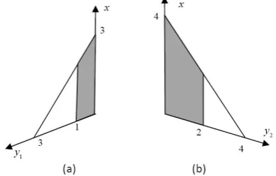
The leader’s constraint region can be shown in the fig. 1 and the constraint regions of the first follower and the second follower are respectively presented at the Fig.2 and Fig.3.
Fig. 1. The leader’s constraint region.
As it is viewed in the figures, The leader’s and each followers’ constraint region are nonempty and compact, thus first we are able to convert (5.9) to a linear BLMFP problem by using the method in section 2. So, the following problem can be set easily.
max x∈X,λ λ
s.t x+ 2y1+ 3y2 ≤6
y1 ≤2
x+ 2y1+ 3y2−2λ≥4
y1−y2−2λ≥0
0≤λ≤1 max
y1∈Y1,λ1
λ1
s.t x+y1≤3
y1 ≤1
x+y1−2λ1≥1
y1−λ1 ≥0
0≤λ1 ≤1
max y2∈Y2,λ2
λ2
s.t x+y2≤4
y2 ≤2
x+y2−2λ2≥2
y2−2λ2 ≥0
0≤λ2 ≤1
(5.10)
the Kth-best approach, the example can be rewritten as follows:
max x∈X,λ λ
s.t x+ 2y1+ 3y2 ≤6
y1 ≤2
x+ 2y1+ 3y2−2λ≥4
y1−y2−2λ≥0
0≤λ≤1
x+y1≤3
y1 ≤1
x+y1−2λ1 ≥1
y1−λ1 ≥0
0≤λ1≤1
x+y2≤4
y2 ≤2
x+y2−2λ2 ≥2
y2−2λ2 ≥0
0≤λ2≤1
Step 1, set q = 1 and solve the above problem with the simplex method to obtain the optimal solution
Let W = (2,1,0.25,0.375,0,0) and T =∅. Go to Step 2.
Iteration 1:
Setting i←1 and by (3.7), we have
max λ1
s.t x+ 2y1+ 3y2≤6
y1 ≤2
x+ 2y1+ 3y2−2λ≥4
y1−y2−2λ≥0
0≤λ≤1
x+y1 ≤3
y1≤1
x+y1−2λ1 ≥1
y1−λ1 ≥0
0≤λ1 ≤1
x+y2 ≤4
y2≤2
x+y2−2λ2 ≥2
y2−2λ2≥0
0≤λ2 ≤1
x= 2
λ= 0.375
Using the simplex method we have (ye1,eλ1) = (1,1) . Because(ye1,eλ1)̸= (y1[1], λ [1]
1 ) we go
to Step 3. we have
W[1] ={(2,1,0.25,0.375,0,0),(2,1,0.25,0.375,1,0),(2,1,0.25,0.375,0,0.125)
,(2,1,0.667,0.167,0,0),(2,1,0,0,0,0),(1.667,1,0.333,0.333,0,0),(2.75,0.25,0.25,0,0,0)}
and T ={(2,1,0.25,0.375,0,0)} thus
W ={(2,1,0.25,0.375,1,0),(2,1,0.25,0.375,0,0.125),(2,1,0.667,0.167,0,0),(2,1,0,0,0,0)
,(1.667,1,0.333,0.333,0,0),(2.75,0.25,0.25,0,0,0)}
Then go to Step 4. Updateq = 2 and choose
then go to Step 2.
Iteration 2:
Setting i←1 and by (3.7), we have
max λ1
s.t x+ 2y1+ 3y2≤6
y1 ≤2
x+ 2y1+ 3y2−2λ≥4
y1−y2−2λ≥0
0≤λ≤1
x+y1 ≤3
y1 ≤1
x+y1−2λ1 ≥1
y1−λ1 ≥0
0≤λ1 ≤1
x+y2 ≤4
y2≤2
x+y2−2λ2 ≥2
y2−2λ2≥0
0≤λ2 ≤1
x= 2
Using the simplex method we have (ey1,eλ1) = (1,1) . Because (ey1,eλ1) = (y[1]1 , λ [1]
1 ) setting
i←i+ 1 and by (3.7) we have
max λ2
s.t x+ 2y1+ 3y2≤6
y1≤2
x+ 2y1+ 3y2−2λ≥4
y1−y2−2λ≥0
0≤λ≤1
x+y1≤3
y1≤1
x+y1−2λ1≥1
y1−λ1≥0
0≤λ1≤1
x+y2≤4
y2≤2
x+y2−2λ2≥2
y2−2λ2≥0
0≤λ2≤1
x= 2
λ= 0.375
Using the simplex method we have (ey2,eλ2) = (0.25,0.125) . Because (ey2,λe2)̸= (y[2]1 , λ [2] 1 )
we should continue the algorithm by Step 3. If we follow the Steps of the algorithm as as be-fore, the optimal solution is obtained at the point(x∗, y∗1, y∗2, λ∗, λ∗1, λ2∗) = (2,1,0.25,0.375,1,0.125) and therefore we get the optimal objective values as follows:
x+ 2y1+ 3y2 = 4.75
y1−y2 = 0.75
x+y1 = 3
y1 = 1
x+y2 = 2.25
y2 = 0.25
6
Conclusion
This paper presented a method to find the global optimal solution of the multi-objective linear bilevel multi-follower programming problems in which there are no sharing variables except the leader’s, by using Fuzzy programming andKth-best algorithm and a numerical example was presented at the end. If the constraint regions of the leader and all the followers are non-empty and compact we are able to solve any linear multi-objective bilevel programming problems.
It might suggest that this approach can be adopted to solve non-linear problems. Also we can use this method for solving MOLBLMFP problems in which there are sharing variables among followers.
References
[1] E. Aiyoshi, K. Shimizu, Hierarchical decentralized systems and its new solution by barrier method, IEEE Transactions on Systems, Man, and Cybernetics. 11 (1981) 444-449.
[2] J. F. Bard, Practical Bilevel Optimization: algorithms and applications, Kluwer Aca-demic Publishers, The Netherlands, USA, (1998).
[3] W. F. Bialas and M. H. Karwan, On two level optimization, IEEE Transactions on Automatic Control. 27 (1982) 211-214.
[4] W. Bialas, M. Karwan, J. Shaw, A parametric complementary pivot approach for two-level linear programming, Technical Report, Operations Research programs, state university of New York at Buffalo, (1980).
[5] W. Bialas, M. Karwan, Multilevel linear programming, Technical Report, State Uni-versity of New York at Biffalo, Operation Research Programm, (1978).
[6] J. Bracken, J. McGill, Mathematical programs with optimization problems in the constraints, Operations Research. 21 (1973) 37-44.
[7] W. Candler, R. Townsley, A linear two-level programming problem, Computers and Operations Research. 9 (1982) 59-76.
[8] S. Dempe, Foundations of Bilevel Programming, Kluwer Academic Publishers, Dordecht, Boston, London, (2002) .
[9] M. H. Farahi and E. Ansari, A new approach to solve Multi-objective linear bilevel programming problems, The Journal of Mathe matics and Computer Science. 1(4) (2010) 313-320.
[10] B. Liu, Stackelberg-Nash equilbrium for multi-level programming with multi-follows using genetic algorithms, Computers math applications. 37(7): (1998) 79-89.
[12] C. Shi, G. Zhang, J. Lu, On the definition of linear bilevel programming solution, Applied Mathematics and Computation. 160 (2005) 169-176.
[13] C. Shi, G. Zhang, J. Lu, An extended Kth-best approach for linear bilevel program-ming, Applied Mathematics and computation. 164 (2005) 843-855.
[14] C. Shi, G. Zhang, JIE LU, The Kth-Best Approach for Linear Bilevel Multi-follower Programming, Journal of Global Optimization. 33 (2005) 563-578.
[15] H. Von Stackelberg, The Theory of the Market Economy, Oxford University Press, York, Oxford, (1952).
[16] D. White, G. Anandalingam, A penalty function approach for solving bilevel linear programs, Journal of Global Optimization. 3 (4) (1993) 397-419.
[17] H. J. Zimmerman, Fuzzy set theory and its applications, Kluwer Academic Publishers, Boston, Dordrecht, London, (1996).